On One Problem of the Nonlinear Convex Optimization

Abstract

In this short paper, we study the problem of traversing a crossbar through a bent channel, which has been formulated as a nonlinear convex optimization problem. The result is a MATLAB code that we can use to compute the maximum length of the crossbar as a function of the width of the channel (its two parts) and the angle between them. In case they are perpendicular to each other, the result is expressed analytically and is closely related to the astroid curve (a hypocycloid with four cusps).

1. Formulation of the Problem

In this paper, we deal with the following problem:

Consider two navigable channels that make an angle $\beta$ with each other having widths $d_1$ and $d_2$. We are to find out what is the longest crossbar (=the line segment, after mathematical abstraction) that can be navigated through this channel! (see Figure 1 for the meaning of the parameters $d_1$, $d_2$ and $\beta$).

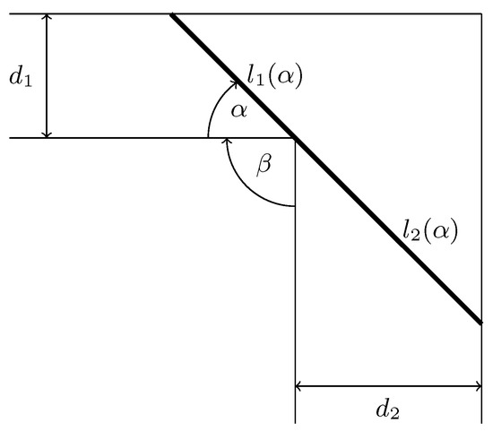
Figure 1. Schematic diagram of the channel.

As we see in a moment, we are able to convert this problem into a convex optimization problem, allowing us to take advantage of its rich and efficient apparatus. The main reasons for focusing on the convex optimization problems are as follows [1]:

-

They are close to being the broadest class of problems we know how to solve efficiently.

-

They enjoy nice geometric properties (e.g., local minima are global).

-

There are excellent softwares that readily solve a large class of convex problems.

-

Numerous important problems in a variety of application domains are convex.

A Brief History of Convex Optimization

In the 19th century, optimization models were used mostly in physics, with the concept of energy as the objective function. No attempt, with the notable exception of Gauss’ algorithm for least squares (y1822), as a result of the most famous dispute in the history of statistics between Gauss and Legendre [2], is made to actually solve these problems numerically.

In the period from 1900 to 1970, an extraordinary effort was made in mathematics to build the theory of optimization. The emphasis was on convex analysis, which allows to describe the optimality conditions of a convex problem. As important milestones in this effort, we can mention [3]:

• 1947: The simplex algorithm for linear programming—the computational tool still prominent in the field today for the solution of these problems (Dantzig [4,5]).
• 1960s: Early interior-point methods (Fiacco and McCormick [6], Dikin [7,8], …).
• 1970s: Ellipsoid method and other subgradient methods, which positively answered the question whether there is another algorithm for linear programming in addition to the simplex method, which has polynomial complexity ([9,10,11,12,13]).
• 1980s: Polynomial-time interior-point methods for linear programming (Karmarkar 1984 [14,15]). From a theoretical point of view, this was a polynomial-time algorithm, in contrast to Dantzig’s simplex method, which in the worst case has exponential complexity [16].
• Late 1980s–now: Polynomial-time interior-point methods for nonlinear convex optimization (Nesterov & Nemirovski 1994 [17,18]).

The growth of convex optimization methods (theory and algorithms) and computational techniques (many algorithms are computationally time-consuming) has led to their widespread application in many areas of science and engineering (control, signal processing, communications, circuit design, and …) and new problem classes (for example, semidefinite and second-order cone programming, robust optimization). For more recent achievements in optimization algorithms, see [19,20,21,22,23] and the references therein.

This paper does not claim to develop new scientific knowledge, but its aim is to use well-known techniques of convex optimization to solve, in my opinion, an interesting practical problem that can also be used in the process of teaching nonlinear convex optimization techniques, and the pedagogical value of the contributions is one of the objectives of this special issue of the journal. The interesting thing about this problem/case study is that there is a naturally occurring minimization problem (without multiplication by a factor of $(-1)$ or similar) when looking for the maximum length.

Now, we introduce the theorem, which is one of the most important theorems in convex analysis [24].

Theorem 1.

Consider an optimization problem

$$\begin{array}{ccc}& & \mathrm{minimize}f\left(x\right)\hfill \\ & & \mathrm{s}.\mathrm{t}.x\in \Omega ,\hfill \end{array}$$

where $f:\Omega \to \mathbb{R}$ is a convex function and $\Omega \subset {\mathbb{R}}^n$ is a convex set. Then, any local minimum is also a global minimum.

2. Analytical and Numerical Solution of the Convex Optimization Problem

In the spirit of the previous considerations, our problem can be formulated as follows:

$$\mathrm{minimize}{l}_{\beta }\left(\alpha \right)=l_1\left(\alpha \right)+l_2\left(\alpha \right)=\frac{d_1}{sin\left(\alpha \right)}+\frac{d_2}{sin\left(\alpha +\beta \right)}\mathrm{s}.\mathrm{t}.-\alpha \le 0,\alpha \le \pi -\beta ,$$

(1)

where $\beta \in (0,\pi )$ is fixed. The angles $\alpha$, $\beta$ are measured in radians, and $d_1$, $d_2$ (both are positive real numbers) are expressed in units of length.

The solution of the problem (1) is hereafter referred to as $l_{\mathrm{maxLength}}\left(\beta \right)$.

The first two derivatives of the function $l_{\beta }\left(\alpha \right)$ are:

$$l_{\beta }^{\prime }\left(\alpha \right)=\frac{d_{1}cos\left(\alpha \right)}{{cos}^2\left(\alpha \right)-1}+\frac{d_{2}cos\left(\alpha +\beta \right)}{{cos}^2\left(\alpha +\beta \right)-1}$$

$$l_{\beta }^{″}\left(\alpha \right)=\frac{2d_1}{{sin}^3\left(\alpha \right)}-\frac{d_1}{sin\left(\alpha \right)}+\frac{2d_2}{{sin}^3\left(\alpha +\beta \right)}-\frac{d_2}{sin\left(\alpha +\beta \right)}$$

$$=\frac{2d_1-d_1{sin}^2\left(\alpha \right)}{{sin}^3\left(\alpha \right)}+\frac{2d_2-d_2{sin}^2\left(\alpha +\beta \right)}{{sin}^3\left(\alpha +\beta \right)}$$

$$\ge \frac{d_1}{{sin}^3\left(\alpha \right)}+\frac{d_2}{{sin}^3\left(\alpha +\beta \right)}>0$$

for all $\alpha \in (0,\pi -\beta )$, and so the function $l_{\beta }\left(\alpha \right)$ is continuous (together with its derivatives) and (strictly) convex on the the convex set $(0,\pi -\beta )\subset \mathbb{R},$ with $l_{\beta }\left(\alpha \right)\to \infty$ for $\alpha \to 0^{+}$ and $\alpha \to {(\pi -\beta )}^{-},$ see also Figure 2 for a better idea of the behavior of the function $l_{\beta }\left(\alpha \right)$. The limits above (both equal to ∞) guarantee the existence, and the strict convexity of the function $l_{\beta }\left(\alpha \right)$ in turns the uniqueness of the local minimum of the function $l_{\beta }\left(\alpha \right)$ on $\Omega$. Theorem 1 says that this local minimum is a solution of the problem (1).

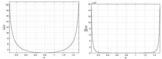
Figure 2. The objective function $l_{\beta }\left(\alpha \right)$ and its second derivative for $\beta =\frac{\pi }{2}$, $d_1=1$ and $d_2=1$ on the interval $[0,\pi -\beta ]$.

For $\beta =\frac{\pi }{2}$, that is, the channel is bent to a right angle, we can compute the value $l_{\mathrm{maxLength}}\left(\frac{\pi }{2}\right)$ analytically:

Theorem 2.

For $\beta =\frac{\pi }{2}$, we have

$$l_{\mathrm{maxLength}}\left(\frac{\pi }{2}\right)={\left(d_1^{\frac{2}{3}}+d_2^{\frac{2}{3}}\right)}^{\frac{3}{2}}.$$

Proof. 

First, using the identity $sin\left(\alpha +\frac{\pi }{2}\right)=cos\left(\alpha \right)$, we obtain from (1)

$$l_{\beta =\pi /2}\left(\alpha \right)=\frac{d_1}{sin\left(\alpha \right)}+\frac{d_2}{cos\left(\alpha \right)},\alpha \in [0,\pi -\beta ]=\left[0,\frac{\pi }{2}\right]$$

(2)

and

$$l_{\beta =\pi /2}^{\prime }\left(\alpha \right)=-\frac{d_1{cos}^3\left(\alpha \right)-d_2{sin}^3\left(\alpha \right)}{{cos}^2\left(\alpha \right){sin}^2\left(\alpha \right)}$$

with the unique stationary point

$${\alpha }^{*}=arctg\left(\sqrt[3]{\frac{d_1}{d_2}}\right),{\alpha }^{*}\in \left(0,\frac{\pi }{2}\right),$$

which is the local minimum of the function $l_{\beta =\pi /2}\left(\alpha \right)$. According to Theorem 1, it holds that

$$l_{\mathrm{maxLength}}\left(\frac{\pi }{2}\right)=l_{\beta =\pi /2}\left({\alpha }^{*}\right).$$

By substituting the value of $\alpha ={\alpha }^{*}$ into the objective function $l_{\beta =\pi /2}\left(\alpha \right)$ defined by (2) and using the basic trigonometry formulas for $x\in \left(-\frac{\pi }{2},\frac{\pi }{2}\right)$ [25]

$$sinx=\frac{\mathrm{tg}x}{\sqrt{1+{\mathrm{tg}}^{2}x}}\mathrm{and}cosx=\frac{1}{\sqrt{1+{\mathrm{tg}}^{2}x}}$$

we obtain

$$l_{\beta =\pi /2}\left({\alpha }^{*}\right)=\frac{d_1\sqrt{1+{\left(\frac{d_1}{d_2}\right)}^{\frac{2}{3}}}}{\sqrt[3]{\frac{d_1}{d_2}}}+d_2\sqrt{1+{\left(\frac{d_1}{d_2}\right)}^{\frac{2}{3}}}$$

$$={\left(d_1^{\frac{2}{3}}+d_2^{\frac{2}{3}}\right)}^{\frac{3}{2}}.$$

   □

Remark 1.

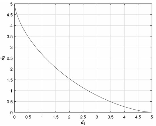
Note that the formula for $l_{\mathrm{maxLength}}\left(\frac{\pi }{2}\right)$ is defined by the astroid curve, its graph for positive values of $d_1$ and $d_2$ is shown in Figure 3. The dependence

$$d_1^{\frac{2}{3}}+d_2^{\frac{2}{3}}=d^{\frac{2}{3}}$$

represents the minimum values of the widths of the two parts of the channel, $d_1$ and $d_2$, for a crossbar of length d to pass through the channel.

Figure 3. The minimum values of $d_1$ and $d_2$ for a 5-unit-long crossbar (d) to pass through the channel (with $\beta =\frac{\pi }{2}$).

Remark 2.

For the limiting values of the parameter β, we obtain, with the obvious interpretation:

$$\beta \to 0^{+}⟹l_{\mathrm{maxLength}}\left(\beta \right)\to (d_1+d_2)(=min\{l_{\beta =0}\left(\alpha \right):\alpha \in [0,\pi ]\})$$

and

$$\beta \to {\pi }^{-}⟹l_{\mathrm{maxLength}}\left(\beta \right)\to \infty (=min\{l_{\beta =\pi }\left(\alpha \right):\alpha =0\}).$$

As an illustrative example, if

$${\beta }_0=1.999999999999\ast \pi /2,d_1=1,d_2=2,$$

then

$$l_{\mathrm{maxLength}}\left({\beta }_0\right)=3710327376774.69.$$

Listing 1 shows the MATLAB code for calculating $l_{\mathrm{maxLength}}\left(\beta \right)$ and Table 1 shows the $l_{\mathrm{maxLength}}\left(\beta \right)$ for the different values of the parameters $d_1$, $d_2$ and $\beta$, indicating the asymptotics of the solved problem, that is, $l_{\mathrm{maxLength}}\left(\beta \right)\to (d_1+d_2)$ for $\beta \to 0^{+}$ and $l_{\mathrm{maxLength}}\left(\beta \right)\to \infty$ for $\beta \to {\pi }^{-}$. The analysis of borderline cases (for us, $\beta$ near 0 and $\pi$), although not of great practical importance, is meaningful from the point of view of mathematical analysis because it points to overall trends in the change in the observed values (here, $l_{\mathrm{maxLength}}\left(\beta \right)$).

Table 1. $l_{\mathrm{maxLength}}\left(\beta \right)$ for the different values of the parameters by employing the code from Listing 1.

	$\mathit{\beta }=\frac{\mathit{\pi }}{100}$	$\mathit{\beta }=\frac{\mathit{\pi }}{6}$	$\mathit{\beta }=\frac{\mathit{\pi }}{4}$	$\mathit{\beta }=\frac{\mathit{\pi }}{2}$	$\mathit{\beta }=\frac{2\mathit{\pi }}{3}$	$\mathit{\beta }=\frac{3\mathit{\pi }}{4}$	$\mathit{\beta }=\frac{99\ast \mathit{\pi }}{100}$
$d_1=1$, $d_2=1$	2.00	2.07	2.16	2.82	4.00	5.22	127.32
$d_1=1$, $d_2=3$	4.00	4.10	4.25	5.40	7.54	9.80	237.60
$d_1=1$, $d_2=5$	6.00	6.12	6.29	7.77	10.69	13.84	333.35
$d_1=2$, $d_2=7$	9.00	9.22	9.54	12.01	16.70	21.69	524.70
$d_1=2$, $d_2=9$	11.00	11.23	11.58	14.38	19.84	25.71	620.27
$d_1=2$, $d_2=11$	13.00	13.24	13.60	16.70	22.90	29.61	712.44

Listing 1. MATLAB code used for calculating $l_{\mathrm{maxLength}}\left(\beta \right)$ for $d_1=1$, $d_2=2$ and $\beta =\frac{\pi }{2}$.

syms alpha beta d1 d2

d1 = 1; % width of the first channel

d2 = 2; % width of the second channel

beta = pi/2; % an angle between the navigable channels

l = (d1/sin(alpha))+(d2/sin(alpha+beta)); % the cost function from (1)

la = diff(l,alpha);

eqn = la == 0;

num = vpasolve(eqn,alpha,[0 pi-beta]); % numerical solver

solution_max_length = simplify(subs(l,num),’Steps’,20) % output

Listing 1. MATLAB code used for calculating $l_{\mathrm{maxLength}}\left(\beta \right)$ for $d_1=1$, $d_2=2$ and $\beta =\frac{\pi }{2}$.

syms alpha beta d1 d2

d1 = 1; % width of the first channel

d2 = 2; % width of the second channel

beta = pi/2; % an angle between the navigable channels

l = (d1/sin(alpha))+(d2/sin(alpha+beta)); % the cost function from (1)

la = diff(l,alpha);

eqn = la == 0;

num = vpasolve(eqn,alpha,[0 pi-beta]); % numerical solver

solution_max_length = simplify(subs(l,num),’Steps’,20) % output

3. Conclusions

The purpose of the present paper is to solve the practical problem of channel navigability and to calculate the maximum length of a crossbar (a line segment, after mathematical abstraction) that will pass through a bent channel. As it turns out, this problem can be formulated as a convex optimization problem. Moreover, of interest is the relationship between the values of $d_1$, $d_2$ and d (the width of the channel sections and the maximum length of the navigable crossbar, respectively), where these values for $\beta =\pi /2$ represent the first-quadrant portion of the astroid curve $d_1^{\frac{2}{3}}+d_2^{\frac{2}{3}}=d^{\frac{2}{3}}$. In the future, it would certainly be interesting to derive an analogous analytical relationship (if it exists) for other values of the $\beta$ angle ($0<\beta <\pi$).

From the future development prospects, the proposed approach could be extended, for example, for solving fuzzy linear programming, fuzzy transportation and fuzzy shortest path problems and DEA models [26,27].

References

- Ahmadi, A.A. Princeton University. 2015. Available online: https://www.princeton.edu/~aaa/Public/Teaching/ORF523/S16/ORF523_S16_Lec4_gh.pdf (accessed on 10 August 2022).
- Stigler, S.M. Gauss and the Invention of Least Squares. Ann. Stat. 1981, 9, 465–474. [Google Scholar] [CrossRef]
- Ghaoui, L.E. University of Berkeley. 2013. Available online: https://people.eecs.berkeley.edu/~elghaoui/Teaching/EE227BT/LectureNotes_EE227BT.pdf (accessed on 10 August 2022).
- Dantzig, G. Origins of the simplex method. In A History of Scientific Computing; Nash, S.G., Ed.; Association for Computing Machinery: New York, NY, USA, 1987; pp. 141–151. [Google Scholar]
- Dantzig, G. Linear Programming and Extensions; Princeton University Press: Princeton, NJ, USA, 1963. [Google Scholar]
- Fiacco, A.; McCormick, G. Nonlinear programming: Sequential Unconstrained Minimization Techniques; John Wiley and Sons: New York, NY, USA, 1968. [Google Scholar]
- Dikin, I. Iterative solution of problems of linear and quadratic programming. Sov. Math. Dokl. 1967, 174, 674–675. [Google Scholar]
- Dikin, I. On the speed of an iterative process. Upr. Sist. 1974, 12, 54–60. [Google Scholar]
- Yudin, D.; Nemirovskii, A. Informational complexity and efficient methods for the solution of convex extremal problems. Matekon 1976, 13, 22–45. [Google Scholar]
- Khachiyan, L. A polynomial time algorithm in linear programming. Sov. Math. Dokl. 1979, 20, 191–194. [Google Scholar]
- Shor, N. On the Structure of Algorithms for the Numerical Solution of Optimal Planning and Design Problems. Ph.D. Thesis, Cybernetic Institute, Academy of Sciences of the Ukrainian SSR, Kiev, Ukraine, 1964. [Google Scholar]
- Shor, N. Cut-off method with space extension in convex programming problems. Cybernetics 1977, 13, 94–96. [Google Scholar] [CrossRef]
- Rodomanov, A.; Nesterov, Y. Subgradient ellipsoid method for nonsmooth convex problems. Math. Program. 2022, 1–37. [Google Scholar] [CrossRef]
- Karmarkar, N. A new polynomial time algorithm for linear programming. Combinatorica 1984, 4, 373–395. [Google Scholar] [CrossRef]
- Adler, I.; Karmarkar, N.; Resende, M.; Veiga, G. An implementation of Karmarkar’s algorithm for linear programming. Math. Program. 1989, 44, 297–335. [Google Scholar] [CrossRef]
- Klee, V.; Minty, G. How Good Is the Simplex Algorithm? Inequalities—III; Shisha, O., Ed.; Academic Press: New York, NY, USA, 1972; pp. 159–175. [Google Scholar]
- Nesterov, Y.; Nemirovski, A.S. Interior Point Polynomial Time Methods in Convex Programming; SIAM: Philadelphia, PA, USA, 1994. [Google Scholar]
- Nemirovski, A.S.; Todd, M.J. Interior-point methods for optimization. Acta Numer. 2008, 17, 191–234. [Google Scholar] [CrossRef]
- Nimana, N. A Fixed-Point Subgradient Splitting Method for Solving Constrained Convex Optimization Problems. Symmetry 2020, 12, 377. [Google Scholar] [CrossRef]
- Han, D.; Liu, T.; Qi, Y. Optimization of Mixed Energy Supply of IoT Network Based on Matching Game and Convex Optimization. Sensors 2020, 20, 5458. [Google Scholar] [CrossRef] [PubMed]
- Popescu, C.; Grama, L.; Rusu, C. A Highly Scalable Method for Extractive Text Summarization Using Convex Optimization. Symmetry 2021, 13, 1824. [Google Scholar] [CrossRef]
- Jiao, Q.; Liu, M.; Li, P.; Dong, L.; Hui, M.; Kong, L.; Zhao, Y. Underwater Image Restoration via Non-Convex Non-Smooth Variation and Thermal Exchange Optimization. J. Mar. Sci. Eng. 2021, 9, 570. [Google Scholar] [CrossRef]
- Alfassi, Y.; Keren, D.; Reznick, B. The Non-Tightness of a Convex Relaxation to Rotation Recovery. Sensors 2021, 21, 7358. [Google Scholar] [CrossRef]
- Boyd, S.; Vandenberghe, L. Convex Optimization; Cambridge University Press: Cambridge, UK, 2004. [Google Scholar]
- Bartsch, H.-J.; Sachs, M. Taschenbuch Mathematischer Formeln für Ingenieure und Naturwissenschaftler, 24th ed.; Neu Bearbeitete Auflage; Carl Hanser Verlag GmbH & Co., KG.: Munich, Germany, 2018. [Google Scholar]
- Ebrahimnejad, A.; Verdegay, J.L. An efficient computational approach for solving type-2 intuitionistic fuzzy numbers based Transportation Problems. Int. J. Comput. Intell. Syst. 2016, 9, 1154–1173. [Google Scholar] [CrossRef]
- Ebrahimnejad, A.; Nasseri, S.H. Linear programmes with trapezoidal fuzzy numbers: A duality approach. Int. J. Oper. Res. 2012, 13, 67–89. [Google Scholar] [CrossRef]
Publisher’s Note: MDPI stays neutral with regard to jurisdictional claims in published maps and institutional affiliations. |
© 2022 by the author. Licensee MDPI, Basel, Switzerland. This article is an open access article distributed under the terms and conditions of the Creative Commons Attribution (CC BY) license (https://creativecommons.org/licenses/by/4.0/).