A Generative Adversarial Network Based Autoencoder for Structural Health Monitoring ^†

Abstract

Civil structures, infrastructures and lifelines are constantly threatened by natural hazards and climate change. Structural Health Monitoring (SHM) has therefore become an active field of research in view of online structural damage detection and long term maintenance planning. In this work, we propose a new SHM approach leveraging a deep Generative Adversarial Network (GAN), trained on synthetic time histories representing the structural responses of both damaged and undamaged multistory building to earthquake ground motion. In the prediction phase, the GAN generates plausible signals for different damage states, based only on undamaged recorded or simulated structural responses, thus without the need to rely upon real recordings linked to damaged conditions.

1. Introduction

Bridges, power generation systems, aircrafts, buildings and rotating machinery are only few instances of structural and mechanical systems which play an essential role in the modern society, even if the majority of them are approaching the end of their original design life [1]. Taking into account that their replacement would be unsustainable from an economic standpoint, alternative strategies for early damage detection have been actively developed so to extend the basis service life of those infrastructures. Furthermore, the advent of novel materials whose long-term behaviour is still not fully understood drives the effort for effective Structural Health Monitoring (SHM), resulting in a saving of human lives and resources [1].

SHM consists of three fundamental steps: (i) measurement, at regular intervals, of the dynamic response of the system; (ii) selection of damage-sensitive features from the acquired data; (iii) statistical analysis of those attributes to assess the current health state of the structure. To characterize the damage state of a system, the method relying on hierarchical phases, originally proposed by [2] represents the currently adopted standard. The latter prescribes several consecutive identification phases (to be tackled in order), namely: check the existence of the damage, the location of the damage, its type, extent and the system’s prognosis. Damaged states are identified by comparison with a reference condition, assumed to be undamaged. The detection of the damage location relies upon a wider awareness of the structural behaviour and the way in which it is influenced by damage. This information, along with the knowledge of how the observed features are altered by different kinds of damage, allows to determine the type of damage. The last two phases require an accurate estimation of the damage mechanisms in order to classify its severity and to estimate the Remaining Useful Life (RUL).

All the steps mentioned above rely on continuous data acquisition and processing to obtain information about the current health condition of a system. In the last few years, the concept of Digital Twin has emerged, combining data assimilation, machine learning and physics-based numerical Simulations [1], the latter being essential to completely understand the physics of the structure and damage mechanisms. A suitable tool able to extract main dominant features from a set of data is represented by neural networks [3], especially generative models such as Generative Adversarial Networks (GANs) [4] and Variational Autoencoders (VAEs) [5].

In this paper, an application of the generative neural network RepGAN, proposed by [6], is presented in the context of SHM. Section 2 provides an overview on existing works. In Section 3, the application of RepGAN to Structural Health Monitoring is presented. In Section 4, extensive numerical results are illustrated, while Section 5 gathers some concluding remarks.

2. Related Work

Generative Adversarial Networks [4] are well known due to their generative capability. Given a multidimensional random variable $\mathit{X}\in ({\mathbb{R}}^{d_X},{\mathcal{E}}_X,P_X)$, where $({\mathbb{R}}^{d_X},{\mathcal{E}}_X,P_X)$ denotes the probabilistic space with $\sigma$-algebra ${\mathcal{E}}_X$ and probability measure $P_X$, whose samples are collected in the data set $\mathcal{S}={\left\{{\mathit{x}}^{(i)}\right\}}_{i=1}^N$, with probability density function $p_X(\mathit{X})$, the GAN generator attempts to reproduce synthetic samples $\widehat{\mathit{x}}$, sampled according to the probability density function $p_G(\mathit{X})$ as similar as possible to the original data, i.e., a GAN trains over data samples in order to match $p_G$ with $p_X$. $\mathit{G}$ maps a lower dimension manifold $({\mathbb{R}}^{d_Z},{\mathcal{E}}_Z,P_Z)$ (with $d_Z<d_X$ in general) into the physics space $({\mathbb{R}}^{d_X},{\mathcal{E}}_X,P_X)$. In doing so, $\mathit{G}$ learns to pass the critic test, undergoing the judgement of a discriminator $D:{\mathbb{R}}^{d_X}\to \left[0,1\right]$, simultaneously trained to recognize ${\widehat{\mathit{x}}}^{(i)}$ counterfeits. The adversarial training scheme relies on the following two-players Minimax game:

$$\begin{array}{cc}\hfill \left\{\mathit{G};D\right\}=arg\underset{\mathit{G}}{min}& \underset{D}{max}V(D,\mathit{G})\hfill \\ \hfill V(D,\mathit{G})={\mathbb{E}}_{\mathit{X}\sim p_X}[lnD(\mathit{X})]& +{\mathbb{E}}_{\mathit{Z}\sim p_Z}[ln(1-D(\mathit{G}(\mathit{Z}))]\hfill \end{array}$$

(1)

In practice, $\mathit{G}$ is represented by a neural network ${\mathit{G}}_{\mathit{\theta }}$ and D by a neural network $D_{\mathit{\omega }}$, with trainable weights and biases $\mathit{\theta }$ and $\mathit{\omega }$, respectively. Moreover, $V(D,\mathit{G})$ is approximated by the Empirical Risk function $L_{\mathcal{S}}(\mathit{\omega },\mathit{\theta })$, depending on the data set $\mathcal{S}$, defined as:

$$\begin{array}{cc}\hfill & \left\{\mathit{\theta };\mathit{\omega }\right\}=arg\underset{\mathit{\theta }}{min}\underset{\mathit{\omega }}{max}{L}_{\mathcal{S}}(\mathit{\omega },\mathit{\theta })=\hfill \\ \hfill & =arg\underset{\mathit{\theta }}{min}\underset{\mathit{\omega }}{max}\frac{1}{n}\sum _{i=1}^n\left(ln{D}_{\mathit{\omega }}({\mathit{x}}^{(i)})+ln(1-D_{\mathit{\omega }}({\mathit{G}}_{\mathit{\theta }}({\mathit{z}}^{(i)}))\right)\hfill \end{array}$$

(2)

with ${\mathit{z}}^{(i)}$ sampled from a known latent space probability distribution $p_Z$ (for instance the normal distribution $\mathcal{N}(\mathbf{0},\mathbb{I})$). The generator ${\mathit{G}}_{\mathit{\theta }}$ induces a sampling probability $p_G(\mathit{X};\mathit{\theta })$ so that, when optimized, passes the critic test, with D being unable to distinguish between ${\mathit{x}}^{(i)}$ and ${\mathit{G}}_{\mathit{\theta }}\left({\mathit{z}}^{(i)}\right)$ (i.e., $D({\mathit{x}}^{(i)})=\frac{1}{2}=D({\mathit{G}}_{\mathit{\theta }}\left({\mathit{z}}^{(i)}\right)$). In other words, ${\mathit{x}}^{(i)}$ and ${\mathit{G}}_{\mathit{\theta }}\left({\mathit{z}}^{(i)}\right)$ can be associated with the value of a categorical variable C, with two possible values: class “d” (data) and class “g” (generated). ${\mathit{x}}^{(i)}$ and ${\mathit{G}}_{\mathit{\theta }}\left({\mathit{z}}^{(i)}\right)$ can be therefore sampled with the mixture probability density $p_M=\alpha \chi \left(C=“d”\right)+(1-\alpha )\chi \left(C=\right)$ “g” with $\chi$ being the indicator function and $\alpha =P(C=“d”)$ [7]. The optimum solution of the Minimax game in Equation (2) induces a mixture probability distribution $\frac{1}{2}\left(p_{C=“d”}+p_{C=“g”}\right)$ [4]. The saddle point of $V(D,G)$ corresponds to the minimum (with the respect to to D) of the conditional Shannon’s entropy $\mathbb{S}(C|\mathit{X})$ (see Appendix A). Moreover, minimizing the conditional Shannon’s entropy $\mathbb{S}(C|\mathit{X})$ corresponds to the maximization of the Mutual Information $I(\mathit{X},C)=\mathbb{S}(C)-\mathbb{S}(C|\mathit{X})$ (see Appendix B), i.e., it corresponds to extract $\mathit{X}$ samples ${\mathit{x}}^{(i)}$ or ${\widehat{\mathit{x}}}^{(i)}$ that are indistinguishable (belonging to same class), with an uninformative mapping $\mathit{X}\to C$.

GANs proved useful in various applications such as generation of artificial data for data-set augmentation, filling gaps in corrupted images and image processing. Especially, deep convolutional generative adversarial networks (DCGANs) [8] proved useful in the field of unsupervised learning. SHM could benefit from GANs as they improve the generalisation performance of models, extracting general features from data, as well as their semantics (damage state, frequency content, etc). However, the adversarial training scheme in Appendix C does not grant a bijective mapping ${\mathit{G}}_{{\mathit{\theta }}_Z}:\mathit{Z}\to \mathit{X}$ (decoder) and ${\mathit{F}}_{{\mathit{\theta }}_X}:\mathit{X}\to \mathit{Z}$ (encoder), which is crucial in order to obtain a unique representation of the data into the latent manifold. Autoencoders have been developed for image reconstruction so to learn the identity operator ${\widehat{\mathit{x}}}^{(i)}=\mathcal{I}({\mathit{x}}^{(i)})={\mathit{G}}_{{\mathit{\theta }}_Z}\circ {\mathit{F}}_{{\mathit{\theta }}_X}({\mathit{x}}^{(i)})$. One can leverage the encoder ${\mathit{F}}_{{\mathit{\theta }}_X}$ representation power to sample points ${\widehat{\mathit{z}}}^{(i)}={\mathit{F}}_{{\mathit{\theta }}_X}({\mathit{x}}^{(i)})$ belonging to the latent manifold ${\Omega }_Z$ and the decoder ${\mathit{G}}_{{\mathit{\theta }}_Z}$ to sample points ${\widehat{\mathit{x}}}^{(i)}={\mathit{G}}_{{\mathit{\theta }}_Z}({\mathit{z}}^{(i)})$ belonging to the latent manifold ${\Omega }_X$ (see Equation (1)). In order to make the learning process of GANs stable across a range of data-sets and to realize higher resolution and deeper generative models, Convolutional Neural Networks (CNNs) are employed to define ${\mathit{F}}_{{\mathit{\theta }}_X}$, ${\mathit{G}}_{{\mathit{\theta }}_Z}$ and the discriminators. ${\mathit{F}}_{{\mathit{\theta }}_X}$ and ${\mathit{G}}_{{\mathit{\theta }}_Z}$ induce sampling probability density functions $q_{Z|X}=\frac{q_{XZ}}{p_X}$ and $p_{X|Z}=\frac{p_{XZ}}{p_Z}$, respectively. $p_X$ is usually unknown (depending on the data-set at stake), but $p_Z$ can be chosen ad hoc (such as, for instance, $\mathcal{N}(\mathbf{0},\mathbb{I})$) in order to get a powerful generative tool for realistic data samples ${\widehat{\mathit{x}}}^{(i)}$. A particular type of Autoencoders, called Variational Autoencoders (VAEs) was introduced by [5], consisting in a probabilistic and generative version of the standard Autoencoder, where the encoder ${\mathit{F}}_{{\mathit{\theta }}_X}$ infers the mean ${\mathit{\mu }}_Z$ and variance ${\mathit{\sigma }}_Z^2$ of the latent manifold. However, the main contribution provided by VAEs is the straightforward approach that allows to reorganize the gradient computation and reduce variance in the gradients labelled reparametrization trick.

Adversarial Autoencoders (AAEs) [9] employ the adversarial learning framework in Equation (1), replacing ${\mathit{G}}_{{\mathit{\theta }}_Z}({\mathit{z}}^{(i)})$ by ${\mathit{G}}_{{\mathit{\theta }}_Z}\circ {\mathit{F}}_{{\mathit{\theta }}_X}({\mathit{x}}^{(i)})$ and adding to the adversarial GAN loss the Mean Square Loss $\parallel {\mathit{x}}^{(i)}-{\mathit{G}}_{{\mathit{\theta }}_Z}\circ {\mathit{F}}_{{\mathit{\theta }}_X}({\mathit{x}}^{(i)}){\parallel }^2$ as an optimization penalty, in order to assure a good reconstruction of the original signal. However, AAEs do not assure a bijective mapping between $({\mathbb{R}}^{d_X},{\mathcal{E}}_X,P_X)$ and $({\mathbb{R}}^{d_Z},{\mathcal{E}}_Z,P_Z)$. In order to achieve the bijection (in a probabilistic sense) between $\left(\mathit{x},\widehat{\mathit{z}}\right)$ and $\left(\widehat{\mathit{x}},\mathit{z}\right)$ samples, the distance between the joint probability distributions $q_{X\widehat{Z}}=q_{\widehat{Z}|X}{p}_X$ and $p_{\widehat{X}Z}=p_{\widehat{X}|Z}{p}_Z$ [10], with the posteriors $q_{\widehat{Z}|X}$ and $p_{Z|\widehat{X}}$ must be minimized. A suitable distance operator for probability distributions is the so called Jensen–Shannon distance ${\mathbb{D}}_{JS}(q_{X\widehat{Z}}||p_{\widehat{X}Z})$, defined as [10]:

$${\mathbb{D}}_{JS}(q_{X\widehat{Z}}||p_{\widehat{X}Z})=\frac{{\mathbb{D}}_{KL}(q_{X\widehat{Z}}||p_M)+{\mathbb{D}}_{KL}(p_{\widehat{X}Z}||p_M)}{2}=\mathbb{S}(p_M)-\mathbb{S}(\mathit{X},\mathit{Z}|M)$$

(3)

with ${\mathbb{D}}_{KL}(p||q)=\mathbb{S}(p||q)-\mathbb{S}(p)$ being the Kullback–Leibler divergence (see Appendix B) and $p_M=\frac{q_{X\widehat{Z}}+p_{\widehat{X}Z}}{2}$ being the mixture probability distribution [7], i.e., the probability of extracting $\left(\mathit{X},\widehat{\mathit{Z}}\right)$ or $\left(\widehat{\mathit{X}},\mathit{Z}\right)$ from a mixed data set, with $\alpha =P(C=“d”)=\frac{1}{2}$ and the entropy of the mixture probability $\mathbb{S}(M)=ln2$. ${\mathbb{D}}_{JS}(q_{X\widehat{Z}}||p_{\widehat{X}Z})$ can be rewritten as:

$$\begin{array}{cc}\hfill {\mathbb{D}}_{JS}(q_{X\widehat{Z}}||p_{\widehat{X}Z})& =\mathbb{S}(p_M)-\frac{1}{2}\left(\mathbb{S}(q_{X\widehat{Z}})+\mathbb{S}(p_{\widehat{X}Z})\right)=\hfill \\ \hfill & =\mathbb{S}(\mathit{X},\mathit{Z})-\mathbb{S}(\mathit{X},\mathit{Z}|M)=\mathbb{S}(M)-\mathbb{S}(M|\mathit{X},\mathit{Z})\hfill \end{array}$$

(4)

The adversarial optimization problem expressed in Equation (1) can be seen as a minimization of the Jensen–Shannon distance for $C\in \left\{“d”,“g”\right\}$:

$$\begin{array}{cc}\hfill {\mathbb{D}}_{JS}(q_{X\widehat{Z}}||p_{\widehat{X}Z})& +ln2=-\mathbb{S}(M|\mathit{X},\mathit{Z})=\hfill \\ \hfill & =\frac{1}{2}{\mathbb{E}}_{\left(\mathit{X},\widehat{\mathit{Z}}\right)\sim q_{XZ}}\left[D\left(\mathit{X},\widehat{\mathit{Z}}\right)\right]+\frac{1}{2}{\mathbb{E}}_{\left(\widehat{\mathit{X}},\mathit{Z}\right)\sim p_{XZ}}\left[1-D\left(\widehat{\mathit{X}},\mathit{Z}\right)\right]\hfill \end{array}$$

(5)

that can be combined with the Autoencoder model in order to obtain the following expression [10,11]:

$$\begin{array}{cc}\hfill & {\mathbb{D}}_{JS}(q_{X\widehat{Z}}||p_{\widehat{X}Z})+ln2={\mathbb{D}}_{JS}(q_{\widehat{Z}|X}{p}_X||p_{\widehat{X}|Z}{p}_Z)+ln2=\hfill \\ \hfill & =\frac{1}{2}\left[{\mathbb{E}}_{\mathit{X}\sim p_X}\left[D\left(\mathit{X},{\mathit{F}}_{{\mathit{\theta }}_X}(\mathit{X})\right)\right]+{\mathbb{E}}_{\mathit{Z}\sim PZ}\left[1-D\left({\mathit{G}}_{{\mathit{\theta }}_Z}(\mathit{Z}),\mathit{Z}\right)\right]\right]\hfill \end{array}$$

(6)

In this context, ${\mathit{F}}_{{\mathit{\theta }}_X}$ learns to map data into a disentangled latent space, generally following the normal distribution, a good reconstruction is not ensured unless the cross-entropy between $\mathit{X}$ and $\mathit{Z}$ is minimized too [12].

Another crucial aspect of generative models is the semantics of the latent manifold. Most of the standard GAN models trained according to Equation (1) employs a simple factored continuous input latent vector $\mathit{Z}$ and does not enforce any restrictions on the way the generator treats it. The individual dimensions of $\mathit{Z}$ do not correspond to semantic features of the data (uninformative latent manifolds) and $\mathit{Z}$ cannot be effectively used in order to perform meaningful topological operations in the latent manifold (e.g., describing neighborhoods) and to associate meaningful labels to it. An information-theoretic extension to GANs, called InfoGAN [13] is able to learn a meaningful and disentangled representations in a completely unsupervised manner: a Gaussian noise $\mathit{Z}$ is associated with a latent code $\mathit{C}$ to capture the characteristic features of the data distribution (for classification purposes). As a consequence, the generator becomes ${\mathit{G}}_{{\mathit{\theta }}_Z}(\mathit{Z},\mathit{C})$ and the corresponding probability distribution $p_G$, whose Mutual Information with the respect to to the latent codes $\mathit{C}$, namely $I(\mathit{C},{\mathit{G}}_{{\mathit{\theta }}_Z}(\mathit{Z},\mathit{C}))$. The latter is forced to be high, penalizing the GAN loss in Equation (1) with the variational lower bound L${}_I$(G,Q), defined by:

$$L_I(G,Q)={\mathbb{E}}_{\mathit{C}\sim p_C,\mathit{X}\sim p_G}\left[lnQ(\mathit{C}|\mathit{X})\right]+\mathbb{S}(\mathit{C})={\mathbb{E}}_{\mathit{X}\sim p_G}{\mathbb{E}}_{\mathit{C}\sim p_{C|X}}\left[ln{q}_{C|X}\right]+\mathbb{S}(\mathit{C})$$

(7)

with $q_{C|X}$ being the probability distribution approximating the real unknown posterior probability distribution $p_{C|X}$ (and represented by the neural network ${\mathit{Q}}_Z$). $L_I(G,Q)$ can be easily approximated via Monte Carlo simulation, and maximized with the respect to to $q_{C|X}$ and $p_G$ via reparametrization trick [13].

$$V_{\mathrm{InfoGAN}}(D,G,Q)=V(D,G)-\lambda L_I(G,Q)$$

(8)

3. Methods

With the purpose of learning a semantically meaningful and disentangled representation of the SHM time-histories, we adopted in this study the architecture called RepGAN, originally proposed in [6]. RepGAN is based on an encoder-decoder structure (both represented by deep CNNs made of stacked 1D convolutional blocks), with a latent space $\mathit{Z}=\left[\mathit{C},\mathit{S},\mathit{N}\right]$. $\mathit{C}\in {\left[0,1\right]}^{d_C}$ a categorical variable representing the damage class(es), with $\mathit{C}\sim p_C$ which is generally chosen as a categorical distribution over $d_C$ classes, i.e., $p_C=\mathrm{Cat}(d_C)$. $\mathit{S}\in {\mathbb{R}}^{d_S}$ is a continuous variable of dimension $d_S$, with $\mathit{S}\sim p_S$, generally $p_S=\mathcal{N}(\mathbf{0},\mathbb{I})$ or the uniform distribution $p_S=\mathcal{U}(-1,1)$. Finally, $\mathit{N}\in {\mathbb{R}}^{d_N}$ is a random noise of $d_N$ independent components, with $\mathit{N}\sim p_N$, generally $p_N\sim \mathcal{N}(\mathbf{0},\mathbb{I})$. RepGAN adopts the conceptual frameworks of VAEs and InfoGAN, combining the learning of two representations $x\to \widehat{z}\to \widehat{x}$ and $z\to \widehat{x}\to \widehat{z}$, respectively. The $x\to \widehat{z}\to \widehat{x}$ scheme must learn to map multiple data instances ${\mathit{x}}^{(i)}$ into their images (via encoder ${\mathit{F}}_{{\mathit{\theta }}_X}$) in a latent manifold ${\widehat{\mathit{z}}}^{(i)}={\mathit{F}}_{{\mathit{\theta }}_X}({\mathit{x}}^{(i)})$ and back into a distinct instance in data space ${\widehat{\mathit{x}}}^{(i)}={\mathit{G}}_{{\mathit{\theta }}_Z}\circ {\mathit{F}}_{{\mathit{\theta }}_X}({\mathit{x}}^{(i)})$ (via decoder ${\mathit{G}}_{{\mathit{\theta }}_Z}$), providing satisfactory results in reconstruction. $z\to \widehat{x}\to \widehat{z}$ maps multiple data latent instances into the same data representation, in order to guarantee impressive generation and clustering performance. Combining the two surjective mappings, in RepGAN the two learning tasks $x\to \widehat{z}\to \widehat{x}$ and $z\to \widehat{x}\to \widehat{z}$ are performed together with shared parameters in order to obtain a bijective mapping $x\leftrightarrow z$. In practice, the training of $z\to \widehat{x}\to \widehat{z}$ is iterated five times more than the $x\to \widehat{z}\to \widehat{x}$. This ability to learn a bidirectional mapping between the input space and the latent space is achieved through a symmetric adversarial process. The Empirical Loss function can be written as:

$$\begin{array}{cc}\hfill & L_S={\mathbb{D}}_{JS}(p_{\widehat{X}|(C,S,N)}||p_X)+{\mathbb{D}}_{JS}(q_{\widehat{C}|X}||p_C)+{\mathbb{D}}_{JS}(q_{\widehat{S}|X}||p_S)+{\mathbb{D}}_{JS}(q_{\widehat{N}|X}||p_N)\hfill \\ \hfill & -{\mathbb{E}}_{p_C}\left[{\mathbb{E}}_{p_{\widehat{X}|C}}\left[ln{q}_{\widehat{C}|X}\right]\right]-{\mathbb{E}}_{p_S}\left[{\mathbb{E}}_{p_{\widehat{X}|S}}\left[ln{q}_{\widehat{S}|X}\right]\right]-{\mathbb{E}}_{p_X}\left[{\mathbb{E}}_{q_{(C,S,N)|X}}\left[ln{p}_{X|(C,S,N)}\right]\right]\hfill \end{array}$$

(9)

with the terms:

• $-{\mathbb{E}}_{p_C}\left[{\mathbb{E}}_{p_{\widehat{X}|C}}\left[ln{q}_{\widehat{C}|X}\right]\right]$ minimizing the conditional entropy $\mathbb{S}(\mathit{C}|\mathit{X})$;
• $-{\mathbb{E}}_{p_S}\left[{\mathbb{E}}_{p_{\widehat{X}|S}}\left[ln{q}_{\widehat{S}|X}\right]\right]$ minimizing the conditional entropy $\mathbb{S}(\mathit{S}|\mathit{X})$.

are introduced in order to constrain a deterministic and injective encoding mapping (see Appendix B). On the other hand, the term

• $-{\mathbb{E}}_{p_X}[{\mathbb{E}}_{q_{(C,S,N)|X}}$$\left[ln{p}_{X|(C,S,N)}\right]]$.

penalizes the learning scheme, in order to minimize the conditional entropy $\mathbb{S}(\mathit{X}|(\mathit{C},\mathit{S},\mathit{N}))$, i.e., in order to grant a good reconstruction.

Following the original RepGAN formulation:

• $-{\mathbb{E}}_{p_X}\left[{\mathbb{E}}_{q_{(C,S,N)|X}}\left[ln{p}_{X|(C,S,N)}\right]\right]$ is enforced penalizing the $L_1$-norm $|\mathit{X}-{\mathit{G}}_{{\mathit{\theta }}_Z}\circ {\mathit{F}}_{{\mathit{\theta }}_X}(\mathit{X})|$;
• ${\mathbb{E}}_{p_S}\left[{\mathbb{E}}_{p_{\widehat{X}|S}}\left[ln{q}_{\widehat{S}|X}\right]\right]$ corresponds to the InfoGAN $L_I$ penalty, and it is maximized via the reparametrization trick (structuring the $\mathit{S}$ branch of the encoder-decoder structure as a VAE, see [5]).

Finally, ${\mathbb{E}}_{p_C}\left[{\mathbb{E}}_{p_{\widehat{X}|C}}\left[ln{q}_{\widehat{C}|X}\right]\right]$ is maximized in a supervised way, considering the actual class of labeled signals ${\mathit{x}}^{(i)}$: ${\mathit{x}}_d^{(i)}$ corresponding to a damaged structure and ${\mathit{x}}_u^{(i)}$ to an undamaged one, respectively. RepGAN provides an informative and disentangled latent space associated with the damage class $\mathit{C}$. The most significant aspect of the approach is the efficiency in generating reasonable signals for different damage states only on the basis of undamaged recorded or simulated structural responses. Both generators ${\mathit{F}}_{{\mathit{\theta }}_X}$, ${\mathit{G}}_{{\mathit{\theta }}_Z}$ and discriminators $D_{{\mathit{\omega }}_X}$, $D_{{\mathit{\omega }}_C}$, $D_{{\mathit{\omega }}_S}$ and $D_{{\mathit{\omega }}_N}$ are parametrized via 1D CNN (and strided 1D CNN), following [8]. Our RepGAN model has been designed using the Keras API, and trained employing a Nvidia Tesla K40 GPU (on the supercomputer Ruche, the cluster of the Mésocentre Moulon of Paris Saclay University).

4. Results and Discussion

In the following, a case study is considered in order to prove the ability of the new architecture to achieve the three fundamental tasks of semantic generation, clustering and reconstruction. The reference example is a shear building subject to an earthquake ground motion whose signals are taken from the STEAD seismic database [14]. STEAD [14] is a high-quality, large-scale, and global data set of local earthquake and non-earthquake signals recorded by seismic instruments. In this work, local earthquake wave forms (recorded at local distances within 350 km of earthquakes) have been considered. Seismic data are constituted by three wave forms of 60 s duration, recorded in east–west, north–south, and up-dip directions, respectively. The structure is composed of 39 storeys. The mass and the stiffness of each floor, in undamaged conditions, are, respectively, m = 625 × 10${}^3$ kg and k = 1 × 10${}^9$ $\frac{kN}{m}$. Damage is simulated through the degradation of stiffness. In the present case, the stiffness reduction has been set equal to 50% of the above mentioned value. The structural response of the system is evaluated considering one degree-of-freedom (dof) per floor. To take into account damping effects, a Rayleigh damping model has been considered.

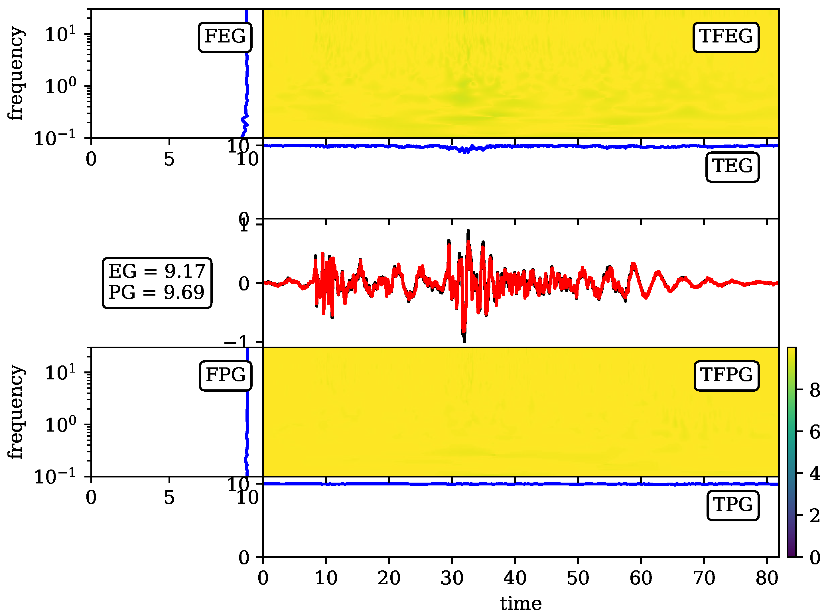
The following results have been obtained considering 100 signals in both undamaged and damaged conditions for a total of 200 samples, with separated training and validation data sets. Each signal is composed of 2048 time steps with dt = 0.04 s. The training process has been performed over 2000 epochs. The reconstruction capability of the proposed network has been evaluated through the Goodness-of-Fit (GoF) criteria [15] where both the fit in Envelope (EG) and the fit in Phase (FG) are measured. An example is shown in Figure 1. The values 9.17 and 9.69, respectively, related to EG and PG testify the excellent reconstruction quality.

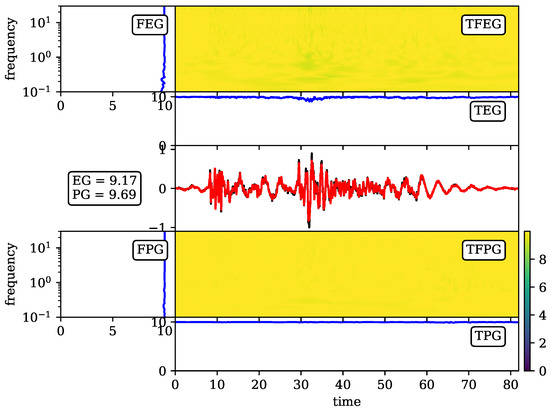
Figure 1. Time–Frequency Goodness-of-Fit criterion: the black line represents the original time-histories ${\mathit{x}}^{(i)}$ while the red time history depicts the result of the RepGAN reconstructions ${\mathit{G}}_Z\circ {\mathit{F}}_X({\mathit{x}}^{(i)})$. GoF is evaluated between 0 and 10: the higher the score, the better is the reconstruction. Frequency Envelope Goodness (FEG), Time–Frequency Envelope Goodness (EG), Time Envelope Goodness (TEG), Frequency Phase Goodness (FPG), Time–Frequency Phase Goodness (PG) and Time Phase Goodness (TPG).

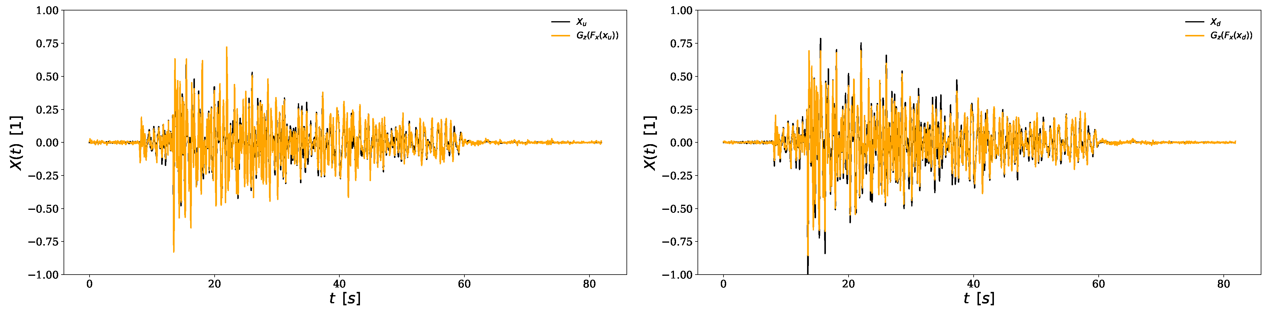
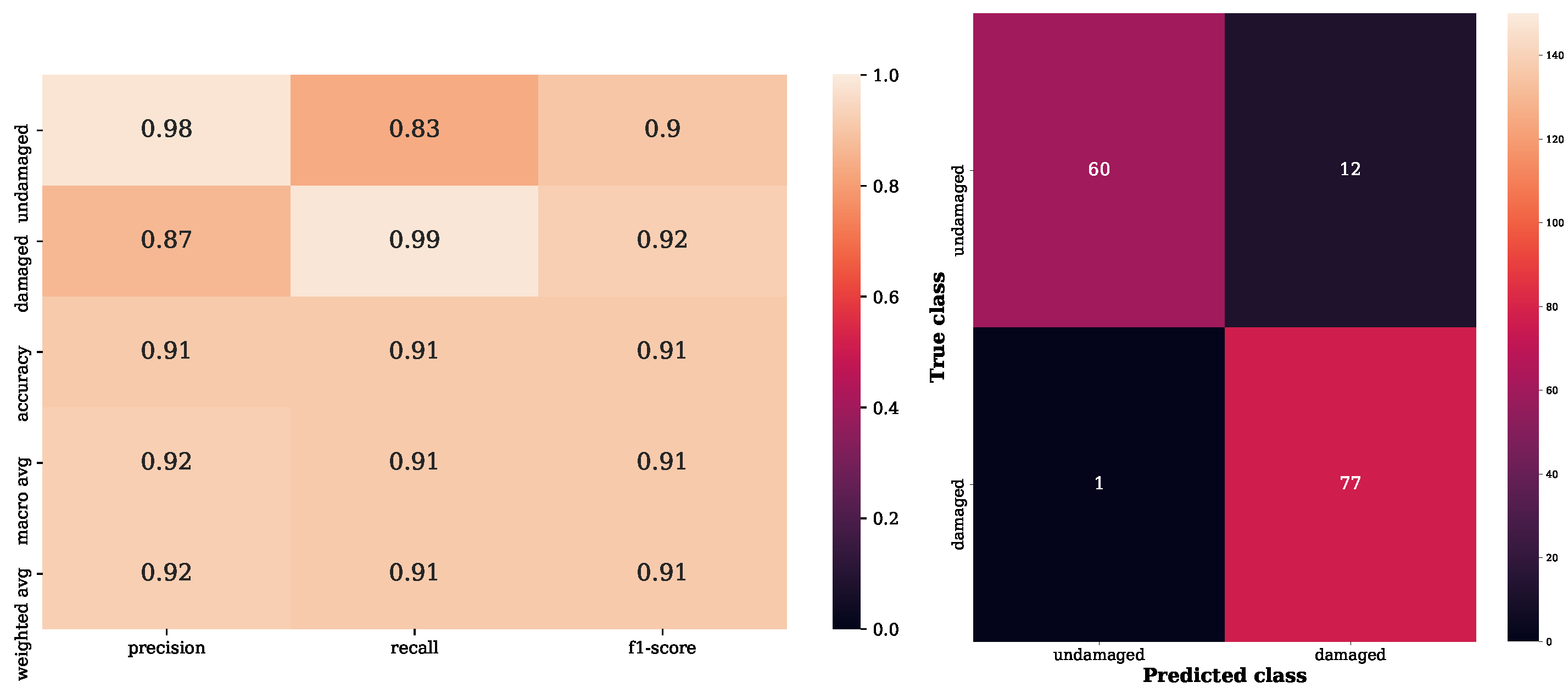
The capability of reproducing signals for different damage scenarios can be appreciated from Figure 2 which presents the original structural response (black) and the corresponding generated one (orange) in both undamaged (left panel in Figure 2) and damaged (right panel in Figure 2) conditions. Regarding the classification capability, the classification report and the confusion matrix in Figure 3 highlight the fact that the model is able to correctly assign the damage class to the considered time histories.

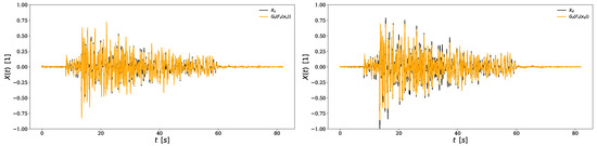
Figure 2. Examples of reconstructed signals for undamaged (left) and damaged (right) time-histories. The black lines represent the original time-histories ${\mathit{x}}_u^{(i)}$ and ${\mathit{x}}_d^{(i)}$, respectively. The orange time histories represent the result of the RepGAN reconstructions ${\mathit{G}}_Z\circ {\mathit{F}}_X({\mathit{x}}_u^{(i)})$ and ${\mathit{G}}_Z\circ {\mathit{F}}_X({\mathit{x}}_d^{(i)})$, respectively. The proposed examples represent the normalized displacement of the 1st floor of the building in object.

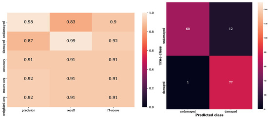
Figure 3. Evaluation of the classification ability of the model. On the left panel, precision, recall, f1-score and accuracy values are reported. A precision score of 1.0 for a class C means that every item labelled as belonging to class C does indeed belong to class C, whereas a recall of 1.0 means that every item from class C was labelled as belonging to class C. F1-score is the harmonic mean of the precision and recall. Accuracy represents the proportion of correct predictions among the total number of cases examined. On the right panel, the confusion matrix allows to visualize the performance of the model: each row of the matrix represents the instances in the actual class, while each column depicts the instances in the predicted class.

5. Conclusions

In this paper, we introduce a SHM method based on a deep Generative Adversarial Network. Trained on synthetic time histories that represent the structural response of a multistory building in both damaged and undamaged conditions, the new model achieves high classification accuracy (Figure 3) and satisfactory reconstruction quality (Figure 1 and Figure 2), resulting in a good bidirectional mapping between the input space and the latent space. However, the major innovation of the proposed method is the ability to generate reasonable signals for different damage states, based only on undamaged recorded or simulated structural responses. As a consequence, real recordings linked to damaged conditions are not requested. In our future work, we would like to extend our approach to real-time data. We will further consider a dataset constituted by a far larger number of time histories.

References

- Farrar, C.R.; Worden, K. Structural Health Monitoring: A Machine Learning Perspective; Wiley: Oxford, UK, 2013. [Google Scholar] [CrossRef] [Green Version]
- Rytter, A. Vibrational Based Inspection of Civil Engineering Structures. Ph.D. Thesis, University of Aalborg, Aalborg, Denmark, 1993. [Google Scholar]
- Bishop, C.M. Neural Networks for Pattern Recognition; Oxford University Press: Oxford, UK, 1995. [Google Scholar]
- Goodfellow, I.J.; Pouget-Abadie, J.; Mirza, M.; Xu, B.; Warde-Farley, D.; Ozair, S.; Courville, A.; Bengio, Y. Generative adversarial nets. In Proceedings of the 28th Annual Conference on Neural Information Processing Systems (NIPS 2014), Montreal, QC, Canada, 8–13 December 2014. [Google Scholar] [CrossRef]
- Kingma, D.P.; Welling, M. Auto-Encoding Variational Bayes. arXiv 2013, arXiv:1312.6114. [Google Scholar]
- Zhou, Y.; Gu, K.; Huang, T. Unsupervised Representation Adversarial Learning Network: From Reconstruction to Generation. In Proceedings of the 2019 International Joint Conference on Neural Networks (IJCNN), Budapest, Hungary, 14–19 July 2019. [Google Scholar] [CrossRef] [Green Version]
- Lindsay, B.G. Mixture Models: Theory, Geometry and Applications. In NSF-CBMS Regional Conference Series in Probability and Statistics; Institute of Mathematical Statistics and American Statistical Association: Suitland, MD, USA, 1995; Volume 5, p. 163. ISBN 0-940600-32-3. [Google Scholar]
- Radford, A.; Luke, L.M.; Chintala, S. Unsupervised Representation Learning with Deep Convolutional Generative Adversarial Networks. arXiv 2015, arXiv:1511.06434. [Google Scholar]
- Makhzani, A.; Shlens, J.; Jaitly, N.; Goodfellow, I. Adversarial Autoencoders. In Proceedings of the International Conference on Learning Representations, San Juan, Puerto Rico, 2–4 May 2016. [Google Scholar]
- Dumoulin, V.; Belghazi, I.; Poole, B.; Mastropietro, O.; Lamb, A.; Arjovsky, M.; Courville, A. Adversarially Learned Inference. arXiv 2016, arXiv:1606.00704v3. [Google Scholar]
- Donahue, J.; Krähenbühl, P.; Darrell, T. Adversarial Feature Learning. arXiv 2017, arXiv:1605.09782. [Google Scholar]
- Li, C.; Liu, H.; Chen, C.; Pu, Y.; Chen, L.; Henao, R.; Carin, L. ALICE: Towards understanding adversarial learning for joint distribution matching. In Proceedings of the 31st International Conference on Neural Information Processing Systems (NIPS’17), Long Beach, CA, USA, 4–9 December 2017; Curran Associates Inc.: Red Hook, NY, USA, 2017; pp. 5501–5509. [Google Scholar]
- Chen, X.; Duan, Y.; Houthooft, R.; Schulman, J.; Sutskever, I.; Abbeel, P. InfoGAN: Interpretable Representation Learning by Information Maximizing Generative Adversarial Nets. In Proceedings of the 30th International Conference on Neural Information Processing Systems, Barcelona, Spain, 5–10 December 2016. [Google Scholar]
- Mousavi, S.M.; Sheng, Y.; Zhu, W.; Beroza, G.C. STanford EArthquake Dataset (STEAD): A Global Data Set of Seismic Signals for AI. IEEE Access 2019, 7, 179464–179476. [Google Scholar] [CrossRef]
- Kristekova, M.; Kristek, J.; Moczo, P. Time-frequency misfit and goodness-of-fit criteria for quantitative comparison of time signals. Geophys. J. Int. 2009, 178, 813–825. [Google Scholar] [CrossRef]
- Vincent, P.; Larochelle, H.; Bengio, Y.; Manzagol, P.-A. Extracting and Composing Robust Features with Denoising Autoencoders. In Proceedings of the 25th International Conference on Machine Learning, Helsinki, Finland, 5–9 July 2008; pp. 1096–1103. [Google Scholar]
- Vincent, P.; Larochelle, H.; Lajoie, I.; Bengio, Y.; Manzagol, P.-A. Stacked Denoising Autoencoders: Learning Useful Representations in a Deep Network with a Local Denoising Criterion. J. Mach. Learn. Res. 2010, 11, 3371–3408. [Google Scholar]
Publisher’s Note: MDPI stays neutral with regard to jurisdictional claims in published maps and institutional affiliations. |
© 2021 by the authors. Licensee MDPI, Basel, Switzerland. This article is an open access article distributed under the terms and conditions of the Creative Commons Attribution (CC BY) license (https://creativecommons.org/licenses/by/4.0/).