A Novel Zero-Truncated Katz Distribution by the Lagrange Expansion of the Second Kind with Associated Inferences

Abstract

In this article, the Lagrange expansion of the second kind is used to generate a novel zero-truncated Katz distribution; we refer to it as the Lagrangian zero-truncated Katz distribution (LZTKD). Notably, the zero-truncated Katz distribution is a special case of this distribution. Along with the closed form expression of all its statistical characteristics, the LZTKD is proven to provide an adequate model for both underdispersed and overdispersed zero-truncated count datasets. Specifically, we show that the associated hazard rate function has increasing, decreasing, bathtub, or upside-down bathtub shapes. Moreover, we demonstrate that the LZTKD belongs to the Lagrangian distribution of the first kind. Then, applications of the LZTKD in statistical scenarios are explored. The unknown parameters are estimated using the well-reputed method of the maximum likelihood. In addition, the generalized likelihood ratio test procedure is applied to test the significance of the additional parameter. In order to evaluate the performance of the maximum likelihood estimates, simulation studies are also conducted. The use of real-life datasets further highlights the relevance and applicability of the proposed model.

1. Introduction

In probability theory, positive discrete distributions called “zero-truncated distributions” are used to model data that exclude zero counts. For instance, the number of times a voter casts a ballot during the general election, the number of journal articles published in various disciplines, the number of stressful events reported by patients, and the length of hospital stay, which must be at least one day. Various zero-truncated discrete distributions, such as the zero-truncated Poisson distribution (ZTPD) (see [1]), zero-truncated negative-binomial distribution (see [2]), zero-truncated Katz distribution (ZTKD) (see [3]), zero-truncated generalized negative-binomial distribution (ZTGNBD) (see [4]), zero-truncated generalized Poisson distribution (see [5]), intervened Poisson distribution (IPD) (see [6]), intervened generalized Poisson distribution (IGPD) (see [7]), a generalization of the Poisson–Sujatha distribution (AGPSD) (see [8]), and zero-truncated discrete Lindley distribution (ZTDLD) (see [9]), have been proposed in the literature to model such count data. In spite of the abundance of practical situations with counting data without zero categories, there is a notable sparseness of zero-truncated discrete distributions in the scientific literature, in contrast to the vast number of classical discrete distributions.

Since the early 1970s, researchers studying discrete distributions seem to have focused more on “Lagrangian distributions”, so named because they are connected to the Lagrange expansions (see [10,11]). The authors in [12] considered the possibility of using Lagrangian distributions to address inferential problems in a random mapping theory. A study in [13] showed that, in certain circumstances, all the discrete Lagrangian distributions converged to the Gaussian distribution and the inverse Gaussian distribution. The authors in [14] proposed certain mixture distributions based on Lagrangian distributions. Recently, Lagrangian distributions were used for turbulent collisional fluid–particle flows (see [15]). A unified method for creating the class of “quasi” distributions, which includes the quasi-binomial, quasi-Polya, quasi-hypergeometric, and several new quasi-distributions, was presented in [16] using the Lagrange expansions. As a result, the distributions arose from Lagrange expansions and have gained traction from both theoretical and applied perspectives.

The Lagrangian distributions of the first kind ($L{D}_1$) and the Lagrangian distributions of the second kind ($L{D}_2$) were the first divisions of the class of Lagrangian distributions. The authors in [13] were the first to present and study the $L{D}_1$. Several Lagrangian distributions have been constructed using the $L{D}_1$, but four fundamental distributions, which are the generalized negative binomial distribution, the generalized geometric series distribution, the generalized Poisson distribution, and the generalized logarithmic series distribution, are of particular note and have proven to be very useful in practical applications (see [4]). The authors in [17] defined a Lagrangian Katz distribution (LKD) using the $L{D}_1$. The author in [18] showed that the LKD was a subclass of the generalized Polya–Eggenberger family of distributions. The authors in [19] obtained the LKD as a limiting distribution of the Markov–Polya distribution. The authors in [20] discussed the application of the LKD to time series data.

On the other hand, the authors in [21,22] conducted extensive research on the $L{D}_2$. The Geeta distribution and its characteristics were derived in [23] based on the $L{D}_2$. The authors in [24] proposed the Dev distribution and some of its applications in queuing theory by using the $L{D}_2$. Ref. [25] proposed the Harish distribution and inferred some of its characteristics, with applications in the branching process and queuing theory based on the $L{D}_2$. Furthermore, the authors in [18] also used the $L{D}_2$ to create the generalized LKD of type two. The competence of the distributions proposed based on the $L{D}_2$ profoundly attracted our team, and as a result, we suggested the Lagrangian version of the ZTPD, the zero-truncated binomial distribution, and the IPD (see [26,27,28]). Moreover, the authors in [24] demonstrated that every member of the $L{D}_2$ was also a member of the $L{D}_1$. Thus, the authors observed from the literature that several members of both $L{D}_1$ and $L{D}_2$ were based on various variants of classical discrete distributions that have thoroughly been explored in the literature. Analogously, we were motivated to fill the sparseness of zero-truncated discrete distributions by considering the probability-generating function (PGF) of the ZTKD and generalizing it through the $L{D}_2$ and so we named the new distribution LZTKD.

An overview of the remaining study sections is provided below: Section 2 provides a brief summary of the Lagrange expansions. The construction of the LZTKD and its statistical features are explored in Section 3 and Section 4, respectively. In Section 5, it is established that the LZTKD belongs to the $L{D}_1$ class. In Section 6, the maximum likelihood (ML) estimation approach is employed to explore the parameter estimation of the LZTKD. The significance of the additional parameter in the LZTKD is evaluated using the likelihood ratio test in Section 7. The simulation results based on the maximum likelihood estimates (MLEs) are included in Section 8. Section 9 provides an empirical illustration of the LZTKD, and Section 10 concludes the article.

2. Some Basic Preliminary Results

In this section, we go over some fundamental concepts, such as the Lagrange expansions at the basis of the $L{D}_1$ and $L{D}_2$, as well as some distributions that belong to the $L{D}_1$ and $L{D}_2$ that have already been published in the literature.

2.1. Lagrange Expansions

Let us first present the Lagrange expansions described in [10,11]. These expansions are described as

$$k_2\left(z\right)=\sum _{y=0}^{\infty }\frac{u^y}{y!}{\left.\left[D^{y-1}\left\{{\left(k_1\left(z\right)\right)}^y{k}_2^{{}^{\prime }}\left(z\right)\right\}\right]\right|}_{z=0}$$

(1)

and

$$\frac{k_2\left(z\right)}{1-\frac{z{k}_1^{\prime }\left(z\right)}{k_1\left(z\right)}}=\sum _{y=0}^{\infty }\frac{u^y}{y!}{\left.\left[D^y\left\{{\left(k_1\left(z\right)\right)}^y{k}_2\left(z\right)\right\}\right]\right|}_{z=0},$$

(2)

where $D^r={\left(\frac{\partial }{\partial z}\right)}^r$ and $z=u{k}_1\left(z\right)$, under the conditions that $k_1\left(z\right)$ and $k_2\left(z\right)$ are two analytic functions of z in [−1,1], which are differentiable with respect to z and such that $k_1\left(0\right)\ne 0$.

These expansions are at the basis of our findings.

2.2. Lagrangian Distribution of the First Kind

Along with the Lagrange expansion given in Equation (1), under the following additional conditions:

$k_1\left(1\right)=k_2\left(1\right)=1$, $k_2\left(0\right)\ge 0$, and

$$D^{y-1}\left[{\left(k_1\left(z\right)\right)}^y{k}_2^{\prime }\left(z\right)\right]{|}_{z=0}\ge 0,$$

for $y=0,1,2,\dots$ in Equation (1), we can define the probability mass function (PMF) of the $L{D}_1$ as

$$\mathrm{P}(Y=y)=\left\{\begin{array}{cc}{k}_2\left(0\right)\hfill & y=0,\hfill \\ \\ {\displaystyle \frac{D^{y-1}\left[{\left(k_1\left(z\right)\right)}^y{k}_2^{\prime }\left(z\right)\right]{|}_{z=0}}{y!}}\hfill & y=1,2,\dots .\hfill \end{array}\right.$$

(3)

The class of Lagrangian distributions given in Equation (3) is sometimes denoted as $L{D}_1(k_1\left(z\right),k_2\left(z\right))$. The corresponding PGF of the PMF given in Equation (3) is indicated as

$$G\left(u\right)=k_2\left(z\right),$$

where $u=\frac{z}{k_1\left(z\right)}$.

The functions $k_1\left(z\right)$ and $k_2\left(z\right)$ are called the transformed function and transformer function, respectively. Some important members belonging to the $L{D}_1$ available in the literature are discussed below.

• Generalized Katz Distribution

A special case of the $L{D}_1$ includes the generalized Katz distribution (GKD) given in [4]. It is generated through the PGF of the Katz distribution (KD). That is, the PMF of the GKD is obtained by applying $k_1\left(z\right)={\left(\frac{1-\alpha z}{1-\alpha }\right)}^{-\frac{\beta }{\alpha }}$ and $k_2\left(z\right)={\left(\frac{1-\alpha z}{1-\alpha }\right)}^{-\frac{\gamma }{\alpha }}$ in Equation (3). Hence, it is given by

$$f_1\left(y\right)=\frac{\frac{\gamma }{\alpha }}{\frac{\gamma +\beta y}{\alpha }+y}{\alpha }^y{(1-\alpha )}^{\frac{\gamma +\beta y}{\alpha }}\left(\genfrac{}{}{0pt}{}{\frac{\gamma +\beta y}{\alpha }+y}{y}\right),y=0,1,2,\dots ,$$

where $\left(\genfrac{}{}{0pt}{}{x}{y}\right)$ is the generalized binomial coefficient, that is, $\left(\genfrac{}{}{0pt}{}{x}{y}\right)=\frac{x(x-1)\dots (x-y+1)}{y!}$, $\gamma >0$, $0<\alpha <1$, and $\beta >0$.

• Generalized Poisson distribution

A special case of the $L{D}_1$ includes the generalized Poisson distribution (GPD) given in [4], which is generated through the PGF of the Poisson distribution. That is, the PMF of the GPD is obtained by applying $k_1\left(z\right)=e^{\alpha (z-1)}$ and $k_2\left(z\right)=e^{\gamma (z-1)}$ in Equation (3). It is thus given by

$$f_2\left(y\right)=\frac{\gamma {(\gamma +\alpha y)}^{y-1}{e}^{-\gamma -\alpha y}}{y!},y=0,1,2,3,\dots ,$$

where $\gamma >0$ and $0<\alpha <1$.

• Generalized Binomial Distribution

A special case of the $L{D}_1$ includes the generalized binomial distribution (GBD) given in [4], which is generated through the PGF of the binomial distribution. That is, the PMF of the GBD is obtained by applying $k_1\left(z\right)={(1-\alpha +\alpha z)}^{\beta }$ and $k_2\left(z\right)={(1-\alpha +\alpha z)}^{\gamma }$ in Equation (3). It is thus indicated as

$$f_3\left(y\right)=\frac{\gamma }{\gamma +\beta y}\left(\genfrac{}{}{0pt}{}{\gamma +\alpha y}{y}\right){\alpha }^y{(1-\alpha )}^{\gamma +\beta y-y},y=0,1,2\dots ,$$

where $0<\alpha <1$, $\gamma >0$ and $\beta <{\alpha }^{-1}$.

2.3. Lagrangian Distribution of the Second Kind

Along with the Lagrange expansion given in Equation (2), under the conditions $k_1\left(1\right)=k_2\left(1\right)=1$, $k_2\left(0\right)\ge 0$, $0<k_1^{{}^{\prime }}\left(1\right)<1$, and

$$(1-k_1^{\prime }\left(1\right))\left[D^y\left\{{\left(k_1\left(z\right)\right)}^y{k}_2\left(z\right)\right\}\right]{|}_{z=0}\ge 0,$$

for $y=0,1,\dots$ in Equation (2), we can define the PMF of the $L{D}_2$ (see [21,29]). Explicitly, it is given by

$$\mathrm{P}(Y=y)=\left\{\begin{array}{cc}(1-k_1^{\prime }\left(1\right))k_2\left(0\right)\hfill & y=0,\hfill \\ \\ {\displaystyle \frac{(1-k_1^{\prime }\left(1\right))D^y\left[{\left(k_1\left(z\right)\right)}^y{k}_2\left(z\right)\right]{|}_{z=0}}{y!}}\hfill & y=1,2,3\dots \hfill \end{array}\right.$$

(4)

The class of Lagrangian distributions given in Equation (4) is sometimes denoted as $L{D}_2(k_1\left(z\right),k_2\left(z\right))$.

The corresponding PGF is given by

$$G\left(u\right)=\frac{(1-k_1^{\prime }\left(1\right))k_2\left(z\right)}{1-\frac{z{k}_1^{\prime }\left(z\right)}{k_1\left(z\right)}},$$

(5)

where $u=\frac{z}{k_1\left(z\right)}$.

In this case, the functions $k_1\left(z\right)$ and $k_2\left(z\right)$ are also called the transformed function and transformer function, respectively. Numerous members of the $L{D}_2$ are available in the literature, some of them are described below.

• Weighted Consul Distribution

A special case of the $L{D}_2$ includes the weighted Consul distribution (WCD) given in [4], which is generated through the PGF of the binomial distribution and an analytic function. That is, the PMF of the WCD is obtained by applying $k_1\left(z\right)=z$ and $k_2\left(z\right)={(1-\alpha +\alpha z)}^{\beta }$ in Equation (4). It is given as

$$f_4\left(y\right)=\left(\genfrac{}{}{0pt}{}{\beta y}{y-1}\right)\left(1-\beta \alpha \right){\alpha }^{y-1}{(1-\alpha )}^{\beta y-y+1},y=1,2,3\dots ,$$

where $0<\alpha <1$ and $\beta <{\alpha }^{-1}$.

• Rectangular–Poisson Distribution

A special case of the $L{D}_2$ includes the rectangular–Poisson distribution (RPD) given in [4], which is generated through the PGF of the rectangular distribution and the PGF of the Poisson distribution. That is, the PMF of the RPD is obtained by applying $k_1\left(z\right)=e^{\alpha (z-1)}$ and $k_2\left(z\right)=\frac{1-z^n}{n(1-z)}$ in Equation (4). Hence, it is expressed as

$$f_5\left(y\right)=\frac{(1-\alpha )e^{-y\alpha }}{n}\sum _{i=0}^a\frac{{\left(y\alpha \right)}^i}{i!},y=0,1,2,\dots ,$$

where $n>0$ is an integer, $a=min(y,n-1)$,  $0<\alpha <1$.

• Rectangular–Binomial Distribution

The rectangular–binomial distribution (RBD) given in [4] is a special case of the $L{D}_2$, which is generated by the PGF of the binomial and rectangular distributions, respectively. That is, the PMF of the RBD is obtained by applying $k_1\left(z\right)={(1-\alpha +\alpha z)}^{\beta }$ and $k_2\left(z\right)=\frac{1-z^n}{n(1-z)}$ in Equation (4). It is thus obtained as

$$f_6\left(y\right)=\frac{1-\beta \alpha }{n}{(1-\alpha )}^{\beta y}\sum _{i=0}^a\left(\genfrac{}{}{0pt}{}{\beta y}{i}\right){\left(\frac{\alpha }{1-\alpha }\right)}^i,y=0,1,2,\dots ,$$

where $n>0$ is an integer, $a=min(y,n-1)$,  $0<\alpha <1$, and $\beta <{\alpha }^{-1}$.

Given the applications of the Lagrangian distributions generated with various PGFs, it is worthwhile to investigate other horizon Lagrangian distributions that make use of new PGFs. This serves as the amended study distribution, which is displayed below.

3. Lagrangian Zero-Truncated Katz Distribution (LZTKD)

In this section, we adopt the PMF of the $L{D}_2$ given in Equation (4) to derive the PMF of the LZTKD. Here, we consider $k_1\left(z\right)$ as the PGF of the KD with parameters $0<\alpha <1$ and $\beta <1-\alpha$, and $k_2\left(z\right)$ as the PGF of the ZTKD with parameters $0<\alpha <1$ and $\gamma >0$ to generate the LZTKD.

That is, we take

$$k_1\left(z\right)={\left(\frac{1-\alpha z}{1-\alpha }\right)}^{-\frac{\beta }{\alpha }},k_2\left(z\right)=\frac{{\left(\frac{1-\alpha z}{1-\alpha }\right)}^{-\frac{\gamma }{\alpha }}-{\left(1-\alpha \right)}^{\frac{\gamma }{\alpha }}}{1-{\left(1-\alpha \right)}^{\frac{\gamma }{\alpha }}}.$$

(6)

The analytic functions given in Equation (6) satisfy the conditions presented in Section 2.3. That is, we have

$$k_1\left(0\right)={\left(1-\alpha \right)}^{\frac{\beta }{\alpha }}\ne 0,k_1\left(1\right)=k_2\left(1\right)=1,\mathrm{and}{k}_2\left(0\right)=0.$$

Then, under the transformation $z=u{\left(\frac{1-\alpha z}{1-\alpha }\right)}^{-\frac{\beta }{\alpha }}$, the PMF of the $L{D}_2$ given in Equation (4) can be derived as follows:

$$\begin{array}{cc}\hfill f\left(y\right)& =\frac{1-k_1^{{}^{\prime }}\left(1\right)}{y!}{\left.\left\{D^y\left[{\left(k_1\left(z\right)\right)}^y{k}_2\left(z\right)\right]\right\}\right|}_{z=0}\hfill \\ \hfill & =\frac{\left(1-\frac{\beta }{1-\alpha }\right){(y!)}^{-1}}{1-{(1-\alpha )}^{\frac{\gamma }{\alpha }}}\left\{D^y\left[{\left(\frac{1-\alpha z}{1-\alpha }\right)}^{-\frac{\gamma +\beta y}{\alpha }}-{\left(1-\alpha \right)}^{\frac{\gamma }{\alpha }}{\left(\frac{1-\alpha z}{1-\alpha }\right)}^{-\frac{\beta y}{\alpha }}\right]\right\}{|}_{z=0}\hfill \\ \hfill & =\frac{\left(1-\frac{\beta }{1-\alpha }\right){(y!)}^{-1}}{1-{(1-\alpha )}^{\frac{\gamma }{\alpha }}}\left\{D^y{\left[\frac{1-\alpha z}{1-\alpha }\right]}^{-\frac{\gamma +\beta y}{\alpha }}-{\left(1-\alpha \right)}^{\frac{\gamma }{\alpha }}{D}^y{\left[\frac{1-\alpha z}{1-\alpha }\right]}^{-\frac{\beta y}{\alpha }}\right\}{|}_{z=0}\hfill \\ \hfill & =\frac{\left(1-\frac{\beta }{1-\alpha }\right)}{1-{(1-\alpha )}^{\frac{\gamma }{\alpha }}}{\alpha }^y{\left(1-\alpha \right)}^{\frac{\gamma +\beta y}{\alpha }}\left[\left(\genfrac{}{}{0pt}{}{\frac{\gamma +\beta y}{\alpha }+y-1}{y}\right)-\left(\genfrac{}{}{0pt}{}{\frac{\beta y}{\alpha }+y-1}{y}\right)\right],\hfill \end{array}$$

where $\left(\genfrac{}{}{0pt}{}{-n}{m}\right)=\frac{(-n)(-n-1)\dots (-n-m+1)}{m!}$ = ${(-1)}^m\left(\genfrac{}{}{0pt}{}{n+m-1}{m}\right)$.

Hence, the definition of the LZTKD can be formalized as follows:

Definition 1. 

Assume that a random variable (RV) Y follows the LZTKD, with $0<\alpha <1$, $0<\beta <1-\alpha$, and $\gamma >0$. Then, the PMF of Y is given by

$$f\left(y\right)=\frac{\left(1-\frac{\beta }{1-\alpha }\right)}{1-{(1-\alpha )}^{\frac{\gamma }{\alpha }}}{\alpha }^y{\left(1-\alpha \right)}^{\frac{\gamma +\beta y}{\alpha }}\left[\left(\genfrac{}{}{0pt}{}{\frac{\gamma +\beta y}{\alpha }+y-1}{y}\right)-\left(\genfrac{}{}{0pt}{}{\frac{\beta y}{\alpha }+y-1}{y}\right)\right],$$

(7)

with $y=1,2,3\dots$

This distribution is denoted as LZTKD($\alpha ,\beta ,\gamma$), and one can write $Y\sim LZTKD(\alpha ,\beta ,\gamma )$ to inform that Y follows the LZTKD with the parameters $\alpha$, $\beta$, and $\gamma$.

Now, Figure 1 portrays the graphical representation of the PMF of the LZTKD for different parameter values of $\alpha$, $\beta$, and $\gamma$. We see that it is monotonically decreasing for increasing values of the parameters $\alpha$ and $\gamma$, and decreasing the value of the parameter $\beta$ as the value of y increases. In addition, this graph takes on a bell-shaped appearance as the value of y increases if both the $\alpha$ and $\gamma$ parameters increase but the parameter $\beta$ remains constant.

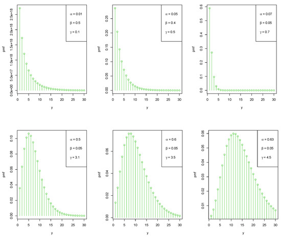
Figure 1. Various shapes of the PMF of the LZTKD for different parameter values.

The hazard rate function (HRF) of the LZTKD is obtained by substituting the PMF in the following equation:

$$\begin{array}{c}\hfill h\left(y\right)=\mathrm{P}(Y=y|Y\ge y)=\frac{f\left(y\right)}{{\sum }_{j=y}^{\infty }f\left(j\right)},y=1,2,3\dots \end{array}$$

(8)

From Equation (8), it goes without saying that determining the closed-form expression of the HRF is more difficult. However, to determine the shape of the HRF, we sketched its graph. Figure 2 demonstrates that it has increasing, decreasing, bathtub, and upside-down bathtub shapes for various parameter values.

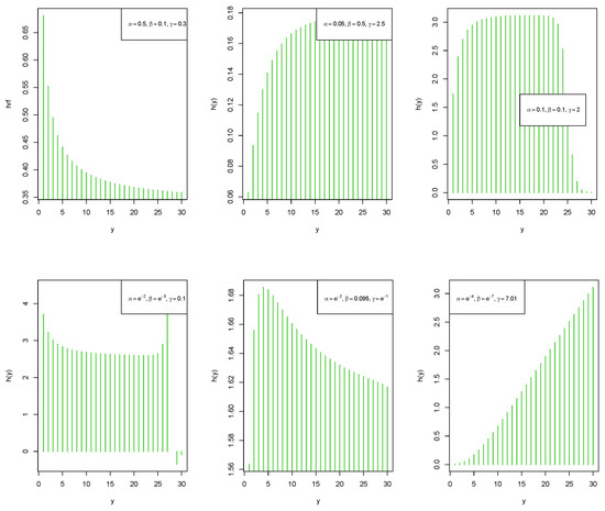
Figure 2. Various shapes of the HRF of the LZTKD for different parameter values.

Proof. 

For $\beta =0$, the LZTKD defined with the PMF given in Equation (7) reduces to the ZTKD; the following PMF is obtained:

$$f\left(y\right)=\frac{\left(\genfrac{}{}{0pt}{}{\frac{\gamma }{\alpha }+y-1}{y}\right){\alpha }^y{(1-\alpha )}^{\frac{\gamma }{\alpha }}}{1-{(1-\alpha )}^{\frac{\gamma }{\alpha }}},y=1,2,3\dots ,$$

In this sense, the LZTKD is a generalization of the ZTKD.    □

Proof. 

For $\beta =0$ in Equation (6), the PMF of the $L{D}_2$ given in Equation (4) can be rederived as follows:

$$\begin{array}{cc}\hfill f\left(y\right)& =\frac{1-k_1^{{}^{\prime }}\left(1\right)}{y!}{\left.\left\{D^y\left[{\left(k_1\left(z\right)\right)}^y{k}_2\left(z\right)\right]\right\}\right|}_{z=0}\hfill \\ \hfill & =\frac{1}{y!}{D}^y{\left.\left[\frac{{\left(\frac{1-\alpha z}{1-\alpha }\right)}^{-\frac{\gamma }{\alpha }}-{(1-\alpha )}^{\frac{\gamma }{\alpha }}}{1-{\left(1-\alpha \right)}^{\frac{\gamma }{\alpha }}}\right]\right|}_{z=0}\hfill \\ \hfill & =\frac{\left(\genfrac{}{}{0pt}{}{\frac{\gamma }{\alpha }+y-1}{y}\right){\alpha }^y{(1-\alpha )}^{\frac{\gamma }{\alpha }}}{1-{(1-\alpha )}^{\frac{\gamma }{\alpha }}},y=1,2,3,\dots ,\hfill \end{array}$$

which is the PMF of the ZTKD given in [3]. The proof is completed.    □

4. Mathematical Properties

In this section, we present some important mathematical properties of the LZTKD, including the median, mode, factorial moments, mean, variance, coefficient of variation (CV), index of dispersion (IOD), skewness, and kurtosis.

4.1. Median

Let Y be a RV following the LZTKD. The median of Y is then defined by the smaller integer $k\in \left\{1,2,3\dots \right\}$ such that $\mathrm{P}(Y\le k)\ge \frac{1}{2}$, also written as

$$\sum _{y=1}^k\left[\left(\genfrac{}{}{0pt}{}{\frac{\gamma +\beta y}{\alpha }+y-1}{y}\right)-\left(\genfrac{}{}{0pt}{}{\frac{\beta y}{\alpha }+y-1}{y}\right)\right]{\alpha }^y{(1-\alpha )}^{\frac{\beta y}{\alpha }}\ge \frac{{(1-\alpha )}^{-\frac{\gamma }{\alpha }}-1}{2\left(1-\frac{\beta }{1-\alpha }\right)}.$$

(9)

4.2. Mode

Let Y be a RV following the LZTKD. Then, the mode of Y, denoted by $y_m$, exists in $\left\{1,2,3\dots \right\}$. It corresponds to the integer y for which the PMF $f\left(y\right)$ has the greatest value. That is, we aim to solve $f\left(y\right)\ge f(y-1)$ and $f\left(y\right)\ge f(y+1)$. First, we note that $f\left(y\right)$ can also be written as

$$f\left(y\right)=\frac{\left(1-\frac{\beta }{1-\alpha }\right)}{1-{(1-\alpha )}^{\frac{\gamma }{\alpha }}}{\alpha }^y{\left(1-\alpha \right)}^{\frac{\gamma +\beta y}{\alpha }}\mathsf{\Lambda }\left(y\right),$$

where $\mathsf{\Lambda }\left(y\right)=\left(\genfrac{}{}{0pt}{}{\frac{\gamma +\beta y}{\alpha }+y-1}{y}\right)-\left(\genfrac{}{}{0pt}{}{\frac{\beta y}{\alpha }+y-1}{y}\right)$.

Obviously, the inequality $f\left(y\right)\ge f(y-1)$ implies that

$$\frac{\mathsf{\Lambda }\left(y\right)}{\mathsf{\Lambda }(y-1)}\ge \frac{1}{\alpha {(1-\alpha )}^{\frac{\beta }{\alpha }}}.$$

(10)

Moreover, the inequality $f\left(y\right)\ge f(y+1)$ implies that

$$\frac{\mathsf{\Lambda }(y+1)}{\mathsf{\Lambda }\left(y\right)}\le \frac{1}{\alpha {(1-\alpha )}^{\frac{\beta }{\alpha }}}.$$

(11)

By combining Equations (10) and (11), we obtain the following condition:

$$\frac{\mathsf{\Lambda }(y_m+1)}{\mathsf{\Lambda }\left(y_m\right)}\le \frac{1}{\alpha {(1-\alpha )}^{\frac{\beta }{\alpha }}}\le \frac{\mathsf{\Lambda }\left(y_m\right)}{\mathsf{\Lambda }(y_m-1)}.$$

(12)

4.3. Probability Generating Function

The Lagrangian transformation $z=u{\left(\frac{1-\alpha z}{1-\alpha }\right)}^{-\frac{\beta }{\alpha }}$, when expanded in powers of u, provides the PGF of the $L{D}_2$ given in Equation (5). That is,

$$\begin{array}{c}\hfill G\left(u\right)=\frac{(1-k_1^{{}^{\prime }}\left(1\right))k_2\left(z\right)}{1-\frac{z{k}_1^{\prime }\left(z\right)}{k_1\left(z\right)}}=\frac{\left(1-\alpha -\beta \right)\left(1-\alpha z\right)\left\{{\left(\frac{1-\alpha z}{1-\alpha }\right)}^{-\frac{\gamma }{\alpha }}-{\left(1-\alpha \right)}^{\frac{\gamma }{\alpha }}\right\}}{\left(1-{\left(1-\alpha \right)}^{\frac{\gamma }{\alpha }}\right)\left\{\frac{(1-\alpha z)-z\beta (1-\alpha )}{(1-\alpha z)}\right\}},\end{array}$$

(13)

where $z=u{\left(\frac{1-\alpha z}{1-\alpha }\right)}^{-\frac{\beta }{\alpha }}$ with $\alpha <1$.

Remark 1. 

The moment-generating function (MGF) of a RV Y following the LZTKD is obtained by putting $z=e^s$ and $u=e^v$ in Equation (13). This yields

$$M\left(v\right)=\mathrm{E}\left(e^{vY}\right)=\frac{\left(1-\alpha -\beta \right)\left(1-\alpha e^s\right)\left\{{\left(\frac{1-\alpha e^s}{1-\alpha }\right)}^{-\frac{\gamma }{\alpha }}-{\left(1-\alpha \right)}^{\frac{\gamma }{\alpha }}\right\}}{\left(1-{\left(1-\alpha \right)}^{\frac{\gamma }{\alpha }}\right)\left\{\frac{(1-\alpha e^s)(1-\alpha )-e^s\beta (1-\alpha )}{(1-\alpha e^s)}\right\}},$$

(14)

where$s=v-\frac{\beta }{\alpha }log\left(\frac{1-\alpha e^s}{1-\alpha }\right)$with$s<-log\alpha$.

4.4. Distribution of Sample Sum

Let $Y_1,Y_2,\dots ,Y_n$ be n independently and identically distributed (iid) RVs following the LZTKD. Then, the distribution of the sample sum $W={\sum }_{i=1}^n{Y}_i$ has the following PGF:

$$\begin{array}{c}\hfill G_1\left(u\right)={\left[\frac{\left(1-\alpha -\beta \right)\left(1-\alpha z\right)\left\{{\left(\frac{1-\alpha z}{1-\alpha }\right)}^{-\frac{\gamma }{\alpha }}-{\left(1-\alpha \right)}^{\frac{\gamma }{\alpha }}\right\}}{\left(1-{\left(1-\alpha \right)}^{\frac{\gamma }{\alpha }}\right)\left\{\frac{(1-\alpha z)-z\beta (1-\alpha )}{(1-\alpha z)}\right\}}\right]}^n,\end{array}$$

where $z=u{\left(\frac{1-\alpha z}{1-\alpha }\right)}^{-\frac{\beta }{\alpha }}$ with $\alpha <1$.

Indeed, based on the PGF of the LZTKD given in Equation (13), the PGF of the RV W becomes

$$\begin{array}{cc}\hfill G_1\left(u\right)& =\mathrm{E}\left(u^W\right)=\mathrm{E}\left(u^{Y_1+Y_2+\dots +Y_n}\right)=\prod _{i=1}^n\mathrm{E}\left(u^{Y_i}\right)=\prod _{i=1}^{n}G\left(u\right)={\left[G\left(u\right)\right]}^n\hfill \\ \hfill & ={\left[\frac{\left(1-\alpha -\beta \right)\left(1-\alpha z\right)\left\{{\left(\frac{1-\alpha z}{1-\alpha }\right)}^{-\frac{\gamma }{\alpha }}-{\left(1-\alpha \right)}^{\frac{\gamma }{\alpha }}\right\}}{\left(1-{\left(1-\alpha \right)}^{\frac{\gamma }{\alpha }}\right)\left\{\frac{(1-\alpha z)-z\beta (1-\alpha )}{(1-\alpha z)}\right\}}\right]}^n.\hfill \end{array}$$

4.5. Factorial Moment

For any integer $r\ge 1$, the rth factorial moments ${\mu }_{\left[r\right]}$ of the LZTKD is calculated by successively differentiating $G\left(u\right)$ in Equation (4) r times with respect to u, and by setting $u=z=1$. Thus, we consider

$$\begin{array}{cc}\hfill G\left(u\right)& =\frac{(1-k_1^{\prime }\left(1\right))k_2\left(z\right)}{(1-u{k}_1^{\prime }\left(z\right))}\hfill \end{array}$$

and

$$\begin{array}{cc}\hfill (1-u{k}_1^{\prime }\left(z\right))G\left(u\right)& =(1-k_1^{\prime }\left(1\right))k_2\left(z\right).\hfill \end{array}$$

Taking the first derivative with respect to u on both sides, we obtain

$$G\left(u\right)D^1(1-u{k}_1^{\prime }\left(z\right))+G^{\prime }\left(u\right)(1-u{k}_1^{\prime }\left(z\right))=(1-k_1^{\prime }\left(1\right))D^1\left(k_2\left(z\right)\right).$$

Then, taking second derivative with respect to u, we obtain

$$G\left(u\right)D^2(1-u{k}_1^{\prime }\left(z\right))+2D^1(1-u{k}_1^{\prime }\left(z\right))G^{\prime }\left(u\right)+(1-u{k}_1^{\prime }\left(z\right))G^{\prime \prime }\left(u\right)=(1-k_1^{\prime }\left(1\right))D^2{k}_2\left(z\right).$$

Proceeding like this, we obtain an rth derivative of the following form:

$$D^r\left(G\left(u\right)\right)=\frac{(1-k_1^{\prime }\left(1\right))D^r\left(k_2\left(z\right)\right)-{\sum }_{i=1}^r(r-i+1)D^{r-i}\left(G\left(u\right)\right)D^i(1-u{k}_1^{\prime }\left(z\right))}{(1-u{k}_1^{\prime }\left(z\right))}.$$

(15)

For $u=z=1$, Equation (15) can be written as

$$\begin{array}{cc}\hfill {\mu }_{\left[r\right]}& =\frac{(1-k_1^{\prime }\left(1\right))D^r\left(k_2\left(z\right)\right)-{\sum }_{i=1}^r(r-i+1){\mu }_{[r-i]}{D}^i(1-u{k}_1^{\prime }\left(z\right))}{(1-u{k}_1^{\prime }\left(z\right))}{\mid }_{u=z=1}\hfill \\ \hfill & =D^r\left(k_2\left(z\right)\right)+\frac{{\sum }_{i=1}^r(r-i+1){\mu }_{[r-i]}{D}^i\left(u{k}_1^{\prime }\left(z\right)\right)}{(1-k_1^{\prime }\left(1\right))}.\hfill \end{array}$$

(16)

We have $k_1\left(z\right)={\left(\frac{1-\alpha z}{1-\alpha }\right)}^{-\frac{\beta }{\alpha }}$ and $k_2\left(z\right)=\frac{{\left(\frac{1-\alpha z}{1-\alpha }\right)}^{-\frac{\gamma }{\alpha }}-{\left(1-\alpha \right)}^{\frac{\gamma }{\alpha }}}{1-{\left(1-\alpha \right)}^{\frac{\gamma }{\alpha }}}$, which are substituted in Equation (16) to yield

$${\mu }_{\left[r\right]}=\frac{D^r{\left(\frac{1-\alpha z}{1-\alpha }\right)}^{-\frac{\gamma }{\alpha }}}{1-{(1-\alpha )}^{\frac{\gamma }{\alpha }}}+\beta \frac{{\sum }_{i=1}^r(r-i+1){\mu }_{[r-i]}{D}^i\left(u{(1-\alpha z)}^{-\frac{\beta }{\alpha }-1}\right)}{\left(1-\frac{\beta }{1-\alpha }\right)}.$$

(17)

4.6. Mean and Variance

The mean (${\mu }_1^{{}^{\prime }}$) and variance (${\sigma }^2$) for the LZTKD are now determined.

Using Equation (17), we have

$$\begin{array}{cc}\hfill {\mu }_1^{{}^{\prime }}=\mathrm{E}\left(Y\right)& =\frac{k_2^{\prime }\left(1\right)}{1-k_1^{\prime }\left(1\right)}+\frac{k_1^{\prime \prime }\left(1\right)+k_1^{\prime }\left(1\right)-{\left(k_1^{\prime }\left(1\right)\right)}^2}{{(1-k_1^{\prime }\left(1\right))}^2}\hfill \\ \hfill & =\frac{\gamma }{\left(1-\alpha -\beta \right)\left(1-{\left(1-\alpha \right)}^{\frac{\gamma }{\alpha }}\right)}+\frac{\beta }{{\left(1-\alpha -\beta \right)}^2}\hfill \end{array}$$

and

$$\begin{array}{cc}\hfill {\sigma }^2& =\mathrm{E}\left(Y(Y-1)\right)+\mathrm{E}\left(Y\right)-{\left(\mathrm{E}\left(Y\right)\right)}^2\hfill \\ & =\frac{k_2^{\prime \prime }\left(1\right)+k_2^{\prime }\left(1\right)-{\left(k_2^{\prime }\left(1\right)\right)}^2}{{(1-k_1^{\prime }\left(1\right))}^2}+\frac{(1+k_2^{\prime }\left(1\right))(k_1^{\prime \prime }\left(1\right)+k_1^{\prime }\left(1\right)-{\left(k_1^{\prime }\left(1\right)\right)}^2)}{{(1-k_1^{\prime }\left(1\right))}^3}\hfill \\ & +\frac{k_1^{\prime \prime \prime }\left(1\right)+k_1^{\prime }\left(1\right)k_1^{\prime \prime }\left(1\right)+2k_1^{\prime \prime }\left(1\right)}{{(1-k_1^{\prime }\left(1\right))}^3}+\frac{2{\left(k_1^{\prime \prime }\left(1\right)\right)}^2}{{(1-k_1^{\prime }\left(1\right))}^4}\hfill \\ \hfill & =\frac{\beta (1-\alpha )(\alpha +\beta +1)}{{(1-\alpha -\beta )}^4}+\frac{{\gamma }^2(1-\alpha -\beta )+\gamma (1-\alpha )}{\left(1-{(1-\alpha )}^{\frac{\gamma }{\alpha }}\right){(1-\alpha -\beta )}^3}-\frac{{\gamma }^2}{{\left(1-{(1-\alpha )}^{\frac{\gamma }{\alpha }}\right)}^2{(1-\alpha -\beta )}^2}.\hfill \end{array}$$

4.7. Index of Dispersion and Coefficient of Variation

A normalized measure of dispersion can be obtained by using the variance-to-mean relationship. This measure, the well-known IOD, is given by

$$\begin{array}{cc}\hfill IOD& =\frac{{\sigma }^2}{{\mu }_1^{{}^{\prime }}}\hfill \\ \hfill & =\frac{\frac{\beta (1-\alpha )(\alpha +\beta +1)}{{(1-\alpha -\beta )}^4}+\frac{{\gamma }^2(1-\alpha -\beta )+\gamma (1-\alpha )}{\left(1-{(1-\alpha )}^{\frac{\gamma }{\alpha }}\right){(1-\alpha -\beta )}^3}-\frac{{\gamma }^2}{{\left(1-{(1-\alpha )}^{\frac{\gamma }{\alpha }}\right)}^2{(1-\alpha -\beta )}^2}}{\frac{\gamma }{\left(1-\alpha -\beta \right)\left(1-{\left(1-\alpha \right)}^{\frac{\gamma }{\alpha }}\right)}+\frac{\alpha +\beta -{\beta }^2}{{\left(1-\alpha -\beta \right)}^2}}.\hfill \end{array}$$

Analogously, the CV of the RV Y has the following form:

$$\begin{array}{cc}\hfill CV& =\frac{\sqrt{{\sigma }^2}}{{\mu }_1^{{}^{\prime }}}\hfill \\ \hfill & =\frac{\sqrt{\frac{\beta (1-\alpha )(\alpha +\beta +1)}{{(1-\alpha -\beta )}^4}+\frac{{\gamma }^2(1-\alpha -\beta )+\gamma (1-\alpha )}{\left(1-{(1-\alpha )}^{\frac{\gamma }{\alpha }}\right){(1-\alpha -\beta )}^3}-\frac{{\gamma }^2}{{\left(1-{(1-\alpha )}^{\frac{\gamma }{\alpha }}\right)}^2{(1-\alpha -\beta )}^2}}}{\frac{\gamma }{\left(1-\alpha -\beta \right)\left(1-{\left(1-\alpha \right)}^{\frac{\gamma }{\alpha }}\right)}+\frac{\alpha +\beta -{\beta }^2}{{\left(1-\alpha -\beta \right)}^2}}.\hfill \end{array}$$

The skewness and kurtosis coefficients of a distribution are frequently used to measure the degree of asymmetry and flatness, respectively. These coefficients are essential to characterize the shape of any distribution, but for the LZTKD, the expressions obtained for such measures were extensive and too lengthy. However, they can be calculated numerically. They are given in Table 1, as well as the mean, variance, CV, and IOD for particular values of the parameters.

Table 1. Mean, variance, CV, IOD, skewness, and kurtosis of the LZTKD for different values of the parameters.

$\mathit{\gamma }$			1	3	5	7	9
$\alpha =0.03$	$\beta =0.7$	Mean	11.9640	20.1849	28.0051	35.5068	42.9319
		Variance	314.2453	393.8855	475.4094	567.9374	664.9710
		IOD	26.2657	19.5138	16.9758	15.9951	15.4889
		CV	1.4816	0.9832	0.7785	0.6711	0.6006
		Skewness	1.3713	1.6726	1.6602	1.2199	1.5408
		Kurtosis	0.8252	2.1227	1.7874	0.2604	0.5978
$\alpha =0.03$	$\beta =0.17$	Mean	1.0627	3.5373	6.4766	9.0084	11.5144
		Variance	5.2686	8.4581	10.7466	13.9438	17.5765
		IOD	4.9575	2.2041	1.6593	1.5478	1.5264
		CV	2.1598	0.7579	0.5061	0.4145	0.3641
		Skewness	3.1290	2.0842	2.2449	2.1332	1.8914
		Kurtosis	3.1408	3.2123	3.1876	2.7445	2.4618
$\alpha =e^{-15}$	$\beta =0.0001$	Mean	1.5722	3.0576	5.0032	6.8921	8.8920
		Variance	2.5651	4.3821	5.3214	7.0245	8.9589
		IOD	1.6315	1.4331	1.0635	1.0192	0.9925
		CV	1.0186	0.6847	0.4610	0.3845	0.3366
		Skewness	1.6415	1.1627	1.4234	1.1610	1.0852
		Kurtosis	2.7316	0.6023	0.4276	0.1721	0.1217

It is clear from this table that for $\alpha >0$ and $\beta >0$, the LZTKD exhibits overdispersion (IOD > 1) and for $\alpha \to 0$ and $\beta \to 0$, the LZTKD exhibits underdispersion (IOD < 1). When the parameter value of $\gamma$ increases, the mean and variance of the LZTKD increases. Moreover, it is noteworthy that the LZTKD has various kurtosis levels and is mainly right-skewed.

5. Relationship Between ${\mathit{LD}}_{\mathit{1}}({\mathit{k}}_{\mathbf{1}}\left(\mathit{z}\right),{\mathit{k}}_{\mathbf{2}}\left(\mathit{z}\right))$ and ${\mathit{LD}}_{\mathbf{2}}({\mathit{k}}_{\mathbf{1}}\left(\mathit{z}\right),{\mathit{k}}_{\mathbf{2}}\left(\mathit{z}\right))$

In this section, we first examine the relationship between the $L{D}_1$ and the $L{D}_2$. Secondly, we show that the LZTKD belongs to the $L{D}_1$.

Theorem 1. 

Let $k_1\left(z\right)=k_2\left(z\right)$ and let X and Y be RVs with distributions into the $L{D}_1\left(k_1\left(z\right),k_2\left(z\right)\right)$ and $L{D}_2\left(k_1\left(z\right),k_2\left(z\right)\right)$, respectively. Then, $\mathrm{P}(Y=t)=(t+1)(1-k_1^{\prime }\left(1\right))\mathrm{P}(X=t)$ for all values of t.

Proof. 

For the PMF of the $L{D}_1$ given in Equation (3) with $k_1\left(z\right)={\left(\frac{1-\alpha z}{1-\alpha }\right)}^{-\frac{\beta }{\alpha }}=k_2\left(z\right)$, we have

$$\begin{array}{cc}\hfill \mathrm{P}(X=t)& =\frac{1}{t!}{\left.\left\{D^{t-1}\left(k_1^t\left(z\right)k_1^{\prime }\left(z\right)\right)\right\}\right|}_{z=0}\hfill \\ \hfill & =\frac{1}{(t+1)!}{D}^t{\left.\left\{\left(k_1^{t+1}\left(z\right)\right)\right\}\right|}_{z=0}\hfill \\ \hfill & =\frac{1}{(t+1)!}{D}^t\left\{{\left(\frac{1-\alpha z}{1-\alpha }\right)}^{-\frac{\beta (t+1)}{\alpha }}\right\}{|}_{z=0}\hfill \\ \hfill & =\frac{{\alpha }^t{(1-\alpha )}^{\frac{\beta (t+1)}{\alpha }}}{(t+1)}\left(\genfrac{}{}{0pt}{}{\frac{\beta (t+1)}{\alpha }+t-1}{t}\right),\hfill \end{array}$$

which belongs to the $L{D}_1$.

For the PMF of the $L{D}_2$ given in Equation (4), we have

$$\begin{array}{cc}\hfill \mathrm{P}(Y=t)& =\frac{(1-k_1^{\prime }\left(1\right))}{t!}{\left.\left\{D^t\left(k_1^t\left(z\right)k_1^{\prime }\left(z\right)\right)\right\}\right|}_{z=0}\hfill \\ \hfill & =\frac{(1-k_1^{\prime }\left(1\right))}{t!}{\left.\left\{D^t\left(k_1^{t+1}\left(z\right)\right)\right\}\right|}_{z=0}\hfill \\ \hfill & =\frac{\left(1-\frac{\beta }{1-\alpha }\right)}{t!}{D}^t\left\{{\left(\frac{1-\alpha z}{1-\alpha }\right)}^{-\frac{\beta (t+1)}{\alpha }}\right\}{|}_{z=0}\hfill \\ \hfill & =\left(1-\frac{\beta }{1-\alpha }\right){\alpha }^t{(1-\alpha )}^{\frac{\beta (t+1)}{\alpha }}\left(\genfrac{}{}{0pt}{}{\frac{\beta (t+1)}{\alpha }+t-1}{t}\right)\hfill \\ \hfill & =(1-k_1^{\prime }\left(1\right))(t+1)\mathrm{P}(X=t).\hfill \end{array}$$

This completes the proof.    □

To show the LZTKD belongs to the $L{D}_1$, we adopt the following equivalence theorem given in [24], also discussed in [4].

Theorem 2. 

Let $k_1\left(z\right)$, $k_2\left(z\right)$, and $k_3\left(z\right)$ be three analytical functions, which are successively differentiable for $\left|z\right|\le 1$ and such that $k_1\left(0\right)\ne 0$ and $k_1\left(1\right)=k_2\left(1\right)=k_3\left(1\right)=1$. Then, under the transformation $z=u{k}_1\left(z\right)$, every member of the $L{D}_2$ is a member of the $L{D}_1$ by choosing

$$k_3\left(z\right)={\left(1-k_1^{{}^{\prime }}\left(1\right)\right)}^{-1}\left(1-\frac{z{k}_1^{{}^{\prime }}\left(z\right)}{k_1\left(z\right)}\right)k_2\left(z\right).$$

(18)

Proof. 

The proof is not new; it is given in [4] and hence omitted.    □

Proof. 

The LZTKD belongs to the $L{D}_1$ by choosing

$$k_3\left(z\right)={\left(1-\frac{\beta }{1-\alpha }\right)}^{-1}\left(1-\frac{z\beta }{1-z\alpha }\right)\left(\frac{{\left(\frac{1-\alpha z}{1-\alpha }\right)}^{-\frac{\gamma }{\alpha }}-{\left(1-\alpha \right)}^{\frac{\gamma }{\alpha }}}{1-{\left(1-\alpha \right)}^{\frac{\gamma }{\alpha }}}\right).$$

   □

Proof. 

For the $L{D}_2(k_1\left(z\right),k_3\left(z\right))$, the PMF can be rewritten as

$$\begin{array}{cc}\hfill \mathrm{P}(Y=y)& ={(y!)}^{-1}(1-k_1^{{}^{\prime }}\left(1\right))D^y\left\{{\left(k_1\left(z\right)\right)}^y{k}_3\left(z\right)\right\}{|}_{z=0}\hfill \\ \hfill & ={(y!)}^{-1}\left(1-\frac{\beta }{1-\alpha }\right)\times \hfill \\ & D^y\left\{{\left(\frac{1-\alpha z}{1-\alpha }\right)}^{-\frac{\beta y}{\alpha }}{\left(1-\frac{\beta }{1-\alpha }\right)}^{-1}\left(1-\frac{z\beta }{1-z\alpha }\right)\left(\frac{{\left(\frac{1-\alpha z}{1-\alpha }\right)}^{-\frac{\gamma }{\alpha }}-{\left(1-\alpha \right)}^{\frac{\gamma }{\alpha }}}{1-{\left(1-\alpha \right)}^{\frac{\gamma }{\alpha }}}\right)\right\}{|}_{z=0}\hfill \\ \hfill & ={(y!)}^{-1}{D}^y\left\{{\left(\frac{1-\alpha z}{1-\alpha }\right)}^{-\frac{\beta y}{\alpha }}\left(1-\frac{z\beta }{1-z\alpha }\right)\left(\frac{{\left(\frac{1-\alpha z}{1-\alpha }\right)}^{-\frac{\gamma }{\alpha }}-{\left(1-\alpha \right)}^{\frac{\gamma }{\alpha }}}{1-{\left(1-\alpha \right)}^{\frac{\gamma }{\alpha }}}\right)\right\}{|}_{z=0}\hfill \\ \hfill & =\left(\frac{\frac{\gamma }{\beta }}{\frac{\gamma +\beta y}{\beta }+y}\right)\left(\genfrac{}{}{0pt}{}{\frac{\gamma +\beta y}{\alpha }+y}{y}\right)\frac{{\alpha }^y{(1-\alpha )}^{\frac{\gamma +\beta y}{\alpha }}}{1-{(1-\alpha )}^{\frac{\gamma }{\alpha }}},y=1,2,3,\dots .\hfill \end{array}$$

It is the same PMF as the one of the zero-truncated generalized Katz distribution (ZTGKD). It is given in [4] and belongs to the $L{D}_1$.    □

6. Estimation of the Parameters

In this section, we estimate the unknown parameters of the LZTKD by the method of the ML.

As a first remark, the model related to the LZTKD is a three-parameter model with parameters $\alpha$, $\beta$, and $\gamma$. Let a random sample of size n be from the LZTKD and let the observed frequency be $n_y$, $y=1,2,3\dots ,k$, so that ${\sum }_{y=1}^k{n}_y=n$, where k is the largest of the observed value having nonzero frequencies. Then, the corresponding likelihood function is given by

$$L=\prod _{y=1}^k{\left\{\frac{\left(1-\frac{\beta }{1-\alpha }\right)}{1-{(1-\alpha )}^{\frac{\gamma }{\alpha }}}{\alpha }^y{\left(1-\alpha \right)}^{\frac{\gamma +\beta y}{\alpha }}\left[\left(\genfrac{}{}{0pt}{}{\frac{\gamma +\beta y}{\alpha }+y-1}{y}\right)-\left(\genfrac{}{}{0pt}{}{\frac{\beta y}{\alpha }+y-1}{y}\right)\right]\right\}}^{n_y}.$$

Thus, the log-likelihood function is obtained as

$$\begin{array}{cc}\hfill {\mathcal{L}}_n=logL& =nlog\left(1-\frac{\beta }{1-\alpha }\right)-nlog\left(1-{(1-\alpha )}^{\frac{\gamma }{\alpha }}\right)+n\overline{y}log\alpha +\frac{n\gamma +\beta n\overline{y}}{\alpha }log(1-\alpha )\hfill \\ & +\sum _{y=1}^k{n}_y\left\{log\left[\prod _{i=0}^{y-1}\left(\frac{\gamma +\beta y}{\alpha }+y-i\right)-\prod _{i=0}^{y-1}\left(\frac{\beta y}{\alpha }+y-i\right)\right]\right\}-\sum _{y=1}^k{n}_{y}log(y!),\hfill \end{array}$$

where $\overline{y}=\frac{1}{n}{\sum }_{y=1}^{k}y{n}_y$.

The maximization of ${\mathcal{L}}_n$ with respect to the parameters gives their respective MLEs. They can also be obtained by considering the following differentiation approach. The score function associated with this log-likelihood function is

$$S\left(v\right)={\left(\begin{array}{ccc}\frac{\partial {\mathcal{L}}_n}{\partial \alpha }& \frac{\partial {\mathcal{L}}_n}{\partial \beta }& \frac{\partial {\mathcal{L}}_n}{\partial \gamma }\end{array}\right)}^T.$$

Now, by solving $\frac{\partial {\mathcal{L}}_n}{\partial \alpha }=0$, $\frac{\partial {\mathcal{L}}_n}{\partial \beta }$=0, and $\frac{\partial {\mathcal{L}}_n}{\partial \gamma }=0$ simultaneously, we obtain the associated nonlinear log-likelihood equations. Consequently, these equations are given by

$$\begin{array}{cc}\hfill \frac{\partial {\mathcal{L}}_n}{\partial \alpha }& =-\frac{n\beta }{(1-\alpha -\beta )(1-\alpha )}-n\frac{\partial \left\{log\left(1-{(1-\alpha )}^{\frac{\gamma }{\alpha }}\right)\right\}}{\partial \alpha }-\left(n\gamma +\beta n\overline{y}\right)\left\{\frac{1}{\alpha (1-\alpha )}+\frac{log(1-\alpha )}{{\alpha }^2}\right\}\hfill \\ \hfill & +\frac{n\overline{y}}{\alpha }+\sum _{y=1}^k{n}_y\frac{\frac{\partial }{\partial \alpha }\left[{\prod }_{i=0}^{y-1}(\frac{\gamma +\beta y}{\alpha }+y-i)-{\prod }_{i=0}^{y-1}(\frac{\beta y}{\alpha }+y-i)\right]}{\left[{\prod }_{i=0}^{y-1}(\frac{\gamma +\beta y}{\alpha }+y-i)-{\prod }_{i=0}^{y-1}(\frac{\beta y}{\alpha }+y-i)\right]}=0,\hfill \end{array}$$

$$\frac{\partial {\mathcal{L}}_n}{\partial \beta }=\frac{n\overline{y}}{\alpha }log(1-\alpha )-\frac{n}{(1-\alpha -\beta )}+\sum _{y=1}^k{n}_y\frac{\frac{\partial }{\partial \beta }\left[{\prod }_{i=0}^{y-1}(\frac{\gamma +\beta y}{\alpha }+y-i)-{\prod }_{i=0}^{y-1}(\frac{\beta y}{\alpha }+y-i)\right]}{\left[{\prod }_{i=0}^{y-1}(\frac{\gamma +\beta y}{\alpha }+y-i)-{\prod }_{i=0}^{y-1}(\frac{\beta y}{\alpha }+y-i)\right]}=0$$

and

$$\begin{array}{cc}\hfill \frac{\partial {\mathcal{L}}_n}{\partial \gamma }& =\frac{n}{\alpha }log(1-\alpha )-n\frac{\partial \left\{log\left(1-{(1-\alpha )}^{\frac{\gamma }{\alpha }}\right)\right\}}{\partial \gamma }\hfill \\ & +\sum _{y=1}^k{n}_y\frac{\frac{\partial }{\partial \gamma }\left[{\prod }_{i=0}^{y-1}(\frac{\gamma +\beta y}{\alpha }+y-i)-{\prod }_{i=0}^{y-1}(\frac{\beta y}{\alpha }+y-i)\right]}{\left[{\prod }_{i=0}^{y-1}(\frac{\gamma +\beta y}{\alpha }+y-i)-{\prod }_{i=0}^{y-1}(\frac{\beta y}{\alpha }+y-i)\right]}=0.\hfill \end{array}$$

Thus, the solutions of these three equations give the MLEs.

In this research, we maximized the log-likelihood function to find the MLEs in the numerical optimization. The fitdistrplus package of RStudio software was used to fix a lower and upper bound for each parameter using the numerical optimization technique “L-BFGS-B”, see [30]. When there are uncertainties about the initial guesses and convergence of the algorithm, fitdistrplus is a highly useful tool that provides original solutions for the MLEs. In order to provide the algorithm with good starting values, we employed the prefit function of that package. Convergence is indicated using certain integer codes as one of the mledist function’s returning components, with “0” denoting a successful convergence and “1” denoting that the maximum number of iterations is used. As a result, a value of “10” indicates that the algorithm is degenerate, and a value of “100” shows that the algorithm made a mistake inside. One can click on the following link for further information about this package https://CRAN.R-project.org/package=fitdistrplus accessed on 3 January 2023. The corresponding R code is given in Appendix A.

7. Likelihood Ratio Test

In this section, we test the significance of an additional parameter included in the LZTKD using the generalized likelihood ratio test (GLRT) (see [31]).

More precisely, to test the significance of the parameter $\beta$ of the LZTKD$(\alpha ,\beta ,\gamma )$, we consider the GLRT procedure. The null hypothesis is that $H_0:Y$ follows the ZTKD against the alternative hypothesis that $H_1:Y$ follows the LZTKD. In this setting, the test statistic is given by

$$-2log{\lambda }^{*}=2\left({\mathcal{L}}_n\left(\hat{\mathsf{\Theta }}\right)-{\mathcal{L}}_n\left({\widehat{\mathsf{\Theta }}}^{*}\right)\right),$$

(19)

where $\widehat{\mathsf{\Theta }}$ is the vector of MLEs of $\mathsf{\Theta }=(\alpha ,\beta ,\gamma )$ with no constraints, and ${\widehat{\mathsf{\Theta }}}^{*}$ is the vector of MLEs of $\mathsf{\Theta }$ under $H_0$. The test statistic presented in Equation (19) is asymptotically distributed as the ${\chi }^2$ distribution with one degree of freedom.

8. Simulation Study

To evaluate the performance of the estimates obtained using the ML estimation approach, we ran a quick simulation exercise in this section. We simulated an LZTKD random sample using the inverse transformation method (see [32]). The following is the inverse transform algorithm for generating a value from the LZTKD:

Step1:

  Generate a random number from the uniform $U(0,1)$ distribution.

Step2:

  $i=1$, $P=\frac{\left(1-\frac{\beta }{\alpha }\right){\left(1-\alpha \right)}^{\frac{\gamma +\beta }{\alpha }}\frac{\gamma }{\alpha }}{1-{\left(1-\alpha \right)}^{\frac{\gamma }{\alpha }}}$, $F=P$.

Step3:

  If $U<F$, set $X=i$ and stop.

Step4:

  $P=P\times \alpha {(1-\alpha )}^{\frac{\beta }{\alpha }}\frac{\left[\left(\genfrac{}{}{0pt}{}{\frac{\gamma +\beta i+1}{\alpha }+i}{i+1}\right)-\left(\genfrac{}{}{0pt}{}{\frac{\beta i+1}{\alpha }+i}{i+1}\right)\right]}{\left[\left(\genfrac{}{}{0pt}{}{\frac{\gamma +\beta i}{\alpha }+i-1}{i}\right)-\left(\genfrac{}{}{0pt}{}{\frac{\beta i}{\alpha }+i-1}{i}\right)\right]}$, $F=F+P$, $i=i+1$.

Step5:

  Go to Step 3.

In the above description, P is the probability that $X=i$, and F is the probability that X is less than or equal to i.

The iteration process was repeated $N=1,000$ times and three parameter sets were considered. The specification of these sets was as follows: 

(i) $\alpha =0.80,\beta =0.03$ and $\gamma =0.80$.

(ii) $\alpha =0.35,\beta =0.09$, and $\gamma =3.12$.

(iii) $\alpha =0.65,\beta =0.03$, and $\gamma =0.51$.  

Thus, we computed the average of the mean square error (MSE), and average absolute bias using the MLEs.

The average absolute bias of the simulated estimates was calculated as $\frac{1}{1000}{\sum }_{i=1}^{1000}|{\widehat{\omega }}_i-\omega |$ and the average MSE of the simulated estimates was calculated as $\frac{1}{1000}{\sum }_{i=1}^{1000}{({\widehat{\omega }}_i-\omega )}^2$, in which i is the number of iterations, $\omega \in \left\{\alpha ,\beta ,\gamma \right\}$ and $\widehat{\omega }$ is the MLE of $\omega$.

Table 2 provides a summary of the study for samples of sizes 50, 250, 500, and 1000. As the sample size increases and for the three parameter sets, it can be seen that the MSEs are in decreasing order, and the MLEs of the parameters become closer to their original parameter values, indicating their consistency property.

Table 2. The simulation for different parameter values $\alpha ,\beta$, and $\gamma$.

Parameter Set	Sample Size	Parameters	Estimates	Absolute Bias	MSE
$\alpha =0.80,\beta =0.03,\gamma =0.80$	$n=50$	$\alpha$	1.1444	0.3444	0.2182
		$\beta$	0.0609	0.0309	0.0009
		$\gamma$	0.5498	0.2001	0.1453
	$n=250$	$\alpha$	1.2254	0.4254	0.1809
		$\beta$	0.0372	0.0072	0.0001
		$\gamma$	0.9256	0.1756	0.0308
	$n=500$	$\alpha$	0.7158	0.0841	0.0505
		$\beta$	0.0360	0.0060	0.00009
		$\gamma$	0.8855	0.1355	0.0227
	$n=1,000$	$\alpha$	0.8120	0.0120	0.0204
		$\beta$	0.0348	0.0048	0.00001
		$\gamma$	0.8121	0.0121	0.0207
$\alpha =0.35,\beta =0.09,\gamma =3.12$	$n=50$	$\alpha$	1.3066	0.9566	0.9459
		$\beta$	0.0647	0.0252	0.0007
		$\gamma$	0.8823	2.2376	5.0122
	$n=250$	$\alpha$	0.9969	0.6469	0.6504
		$\beta$	0.0729	0.0170	0.0007
		$\gamma$	1.7267	1.3932	2.9157
	$n=500$	$\alpha$	1.3129	0.0529	0.0802
		$\beta$	0.0421	0.0078	0.0003
		$\gamma$	1.7452	1.3747	2.8479
	$n=1,000$	$\alpha$	0.3274	0.02025	0.0799
		$\beta$	0.0872	0.0027	0.0005
		$\gamma$	3.4190	0.2990	2.0683
$\alpha =0.65,\beta =0.03,\gamma =0.51$	$n=50$	$\alpha$	1.5121	0.7941	0.7952
		$\beta$	0.0259	0.0089	0.00006
		$\gamma$	0.7954	0.1852	2.2143
	$n=250$	$\alpha$	1.5084	0.7584	0.7369
		$\beta$	0.0227	0.0072	0.00005
		$\gamma$	0.7021	0.1721	0.0369
	$n=500$	$\alpha$	0.9549	0.3049	0.1118
		$\beta$	0.0290	0.0009	0.00003
		$\gamma$	0.5236	0.0136	0.0002
	$n=1,000$	$\alpha$	0.6517	0.0717	0.0072
		$\beta$	0.0301	0.0001	0.00002
		$\gamma$	0.5127	0.0027	0.00001

9. Applications

9.1. Presentation

The purpose of this section is to demonstrate the LZTKD’s empirical relevance. To this end, two COVID-19 datasets were considered. In the first COVID-19 dataset, daily newly reported cases were included, while in the second COVID-19 dataset, daily deaths were included. Since the outbreak’s detection, almost every country has reported at least one new positive case and death each day. To the best of our knowledge, zero-truncated distributions are the most suitable statistical model in this case. In order to show how the LZTKD might be useful, we compared the fits of the various competing distributions, which are presented in Table 3. To evaluate these datasets numerically, we used RStudio software version 4.2.1.

Table 3. The considered competitive distributions.

Distributions	Reference
ZTPD	[1]
IPD	[6]
ZTDLD	[9]
IGPD	[7]
ZTKD	[3]
AGPSD	[8]
ZTGKD	[4]

The HRF of the datasets was determined using a graphical technique based on the total time on test (TTT) plot. If a TTT plot is convex, concave, convex then concave, or concave then convex, the corresponding HRF has a decreasing, increasing, bathtub shape, or an upside-down bathtub shape, respectively (see [33]).

9.2. Daily New Cases of COVID-19 Dataset

Here, we considered a dataset of daily newly reported COVID-19 instances from Algeria in East Africa, recorded between 13 June 2022 to 3 October 2022. These data are accessible at http://covid19.who.int/data, (accessed on 20 October 2022). The dataset is: 2 10 6 9 12 4 3 4 10 8 13 9 10 5 8 11 13 11 14 18 10 13 19 17 17 21 26 18 11 17 29 25 28 36 32 21 42 55 49 63 46 72 67 77 94 86 98 93 87 80 92 111 120 125 131 108 113 102 122 106 134 148 142 133 128 112 92 83 94 81 74 89 77 72 54 48 30 19 41 37 32 55 46 21 17 18 15 13 18 15 10 7 12 10 9 14 15 7 3 3 6 7 6 5 7 4 8 5 8 6 5 3 3.

The descriptive measures of this dataset, which include sample size (n), minimum ($min$), first quartile ($Q_1$), median ($M_d$), third quartile ($Q_3$), maximum ($max$), and interquartile range ($IQR$), are given in Table 4.

Table 4. Descriptive statistics for the COVID-19 dataset from Algeria.

Statistic	n	$\mathit{min}$	${\mathit{Q}}_1$	${\mathit{M}}_{\mathit{d}}$	${\mathit{Q}}_3$	$\mathit{max}$	$\mathit{IQR}$
Values	113	2	10	19	77	148	67

In addition, Figure 3 shows the corresponding empirical TTT plot. It revealed an upside-down bathtub shape HRF.

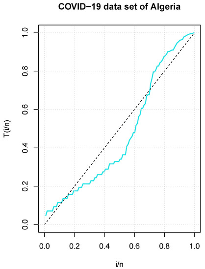
Figure 3. TTT plot for the COVID-19 dataset from Algeria.

We compared the competitive distributions to the LZTKD employing the statistical techniques provided, namely the negative log-likelihood (−$logL$), Akaike information criterion (AIC), Bayesian information criterion (BIC), and ${\chi }^2$ value. Table 5 displays the corresponding MLEs, model adequacy measures, and ${\chi }^2$ values. As it can be seen in this table, the model adequacy measures and ${\chi }^2$ value of the LZTKD are lower than those of the other studied distributions. The suggested model is therefore the most suitable one to model the provided dataset.

Table 5. MLEs, model adequacy measures, and ${\chi }^2$ values for the COVID-19 dataset from Algeria.

Model	MLEs	$-log\mathit{L}$	${\mathit{\chi }}^2$	$\mathbf{df}$	AIC	BIC
ZTPD	$\alpha =42.11645$	2492.831	6752.655	8	4987.661	4990.389
IPD	$\alpha =41.7093$	2492.831	6288.288	7	4989.662	4995.117
	$\beta =0.0102$
ZTDLD	$\alpha =9.7621\times {10}^{-1}$	534.3375	1243.423	7	1072.675	1079.813
	$\beta =5.6811\times {10}^{-5}$
ZTKD	$\alpha =0.0212$	637.6204	5976.975	7	1279.241	1284.696
	$\gamma =0.9556$
AGPSD	$\alpha =0.0464$	553.7651	1214.439	7	1111.530	1116.985
	$\beta =0.00027$
IGPD	$\alpha =1.7271$	580.3144	5395.918	6	1166.629	1174.811
	$\beta =0.7391$
	$\gamma =2.2265$
ZTGKD	$\alpha =0.8527$	532.8011	1325.411	6	1071.602	1079.784
	$\beta =0.0999$
	$\gamma =1.9658$
LZTKD	$\alpha =0.8307$	532.3369	1207.696	6	1070.674	1078.856
	$\beta =0.0999$
	$\gamma =1.3898$

In the case of the GLRT, the calculated value based on the test statistic given in Equation (19) was $2(-532.3369+637.6204)=210.567$ (p-value $=0.03620$). As a result, at any level $>0.03620$, the null hypothesis is rejected in favor of the alternative hypothesis. Hence, we conclude that the additional parameter $\beta$ in the LZTKD is significant in light of the test procedure outlined in Section 7.

9.3. Daily Death Cases of COVID-19 Dataset

Here, we considered a dataset of daily death cases of COVID-19 instances from Bosnia and Herzegovina in Europe, recorded between 2 August 2020 to 28 June 2021. These data are accessible at http://covid19.who.int/data, (accessed on 20 October 2022). The dataset is: 11 12 11 11 6 5 10 8 6 17 22 6 5 11 2 9 6 9 12 8 10 6 5 11 13 11 11 9 3 4 11 11 7 9 3 12 4 9 5 6 5 6 4 6 9 20 11 11 5 6 6 6 8 12 12 6 7 2 12 14 13 5 10 6 2 9 15 5 5 13 1 1 8 11 11 14 8 2 4 11 20 14 20 14 6 15 18 21 36 21 30 22 14 32 37 41 44 55 33 20 73 46 72 49 58 49 41 75 69 47 64 56 40 27 66 52 35 51 62 34 44 61 46 46 39 53 57 30 60 69 70 48 51 48 38 55 66 54 38 34 42 28 53 86 46 40 23 22 30 23 48 26 22 14 14 31 48 32 37 16 21 20 25 28 15 26 12 18 20 23 14 23 12 15 19 14 5 19 28 22 16 20 17 9 19 13 8 16 14 16 9 13 21 19 15 13 11 4 20 19 14 13 17 16 12 9 18 17 11 9 17 8 20 29 29 26 28 19 12 38 48 37 28 36 42 33 63 53 35 57 44 44 48 73 67 62 77 76 58 50 99 74 80 76 88 40 84 66 99 80 84 82 60 47 82 79 76 60 86 49 33 68 87 57 82 39 39 39 69 68 46 48 39 28 15 59 60 23 26 28 21 23 28 50 31 15 23 26 19 25 19 16 10 12 9 14 19 18 16 10 17 11 11 20 17 33 29 42 21 4 12 49 7 6 6 9 3 4 39 74 18 4 4 3 6 5 3 2 2 1 2.

The descriptive measures of the real dataset, which include n, $min$, $Q_1$, $M_d$, $Q_3$, $max$, and $IQR$ are given in Table 6.

Table 6. Descriptive statistics for the COVID-19 dataset from Bosnia and Herzegovina.

Statistic	n	$\mathit{min}$	${\mathit{Q}}_1$	${\mathit{M}}_{\mathit{d}}$	${\mathit{Q}}_3$	$\mathit{max}$	$\mathit{IQR}$
Values	331	1	11	20	43	99	32

In addition, Figure 4 shows an empirical TTT plot for the COVID-19 dataset from Bosnia and Herzegovina and it shows an increasing HRF.

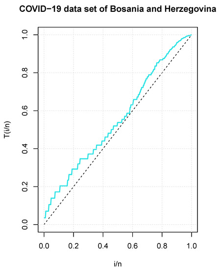
Figure 4. TTT plot for the COVID-19 dataset from Bosnia and Herzegovina.

We used well-established statistical measures to compare the competitive distributions to the LZTKD, including the $-logL$, AIC, BIC, and ${\chi }^2$ value. Table 7 displays the corresponding MLEs, model adequacy measures, and ${\chi }^2$ values. It is observed that the LZTKD’s model adequacy measures and ${\chi }^2$ value are lower than those of the other distributions studied. Because of this, the suggested model is the best choice for modeling the considered dataset.

Table 7. MLEs, model adequacy measures and ${\chi }^2$ values for the Bosnia and Herzegovina COVID-19 dataset.

Model	MLEs	$-log\mathit{L}$	${\mathit{\chi }}^2$	$\mathbf{df}$	AIC	BIC
ZTPD	$\alpha =28.132$	3750.28	2462.098	14	7502.560	7506.363
IPD	$\alpha =2.8134$	3750.28	2451.34	13	7504.56	7512.165
	$\beta =3.3826\times {10}^{-6}$
ZTDLD	$\alpha =0.9444$	1424.361	1692.128	13	2852.721	2863.326
	$\beta =0.0818$
ZTKD	$\alpha =0.0019$	1764.195	8116.362	13	3532.391	3539.995
	$\gamma =0.9626$
AGPSD	$\alpha =6.8867\times {10}^{-2}$	1431.826	1688.206	13	2867.653	2875.257
	$\beta =7.4190\times {10}^{-5}$
IGPD	$\alpha =0.80271$	1424.994	1787.308	12	2855.987	2867.393
	$\beta =0.00036$
	$\gamma =5.5263$
ZTGKD	$\alpha =2.0241\times {10}^{-7}$	1423.018	1692.323	12	2852.035	2863.442
	$\beta =9.5162\times {10}^{-1}$
	$\gamma =1.9658$
LZTKD	$\alpha =0.7915$	1422.617	1684.051	12	2851.234	2862.64
	$\beta =0.0999$
	$\gamma =2.0960$

In the case of the GLRT, the calculated value based on the test statistic given in Equation (19) was $2(-1422.617+1764.195)=341.578$ (p-value $=0.02620$). As a result, at any level $>0.02620$, the null hypothesis is rejected in favor of the alternative hypothesis. Hence, we conclude that the additional parameter $\beta$ in the LZTKD is significant in light of the test procedure outlined in Section 7.

10. Concluding Remarks

In this article, we proposed a novel zero-truncated Lagrangian distribution called the “LZTKD” using the Lagrange expansion of the second kind. We demonstrated that the ZTKD was a special case of the LZTKD. We looked at the shape properties of the PMF and HRF of the LZTKD. The expressions for the factorial moments, generating functions, mean, and median were derived. Using the equivalence theorem of the class of Lagrangian distributions, we demonstrated that the LZTKD belonged to the $L{D}_1$. Subsequently, the ML method was employed to estimate the model parameters for the LZTKD. Using the GLRT procedure, we tested the significance of the additional parameter included in the LZTKD. Simulated studies were conducted to show the effectiveness of MLEs. Two actual datasets were used to validate the results, which proved that the LZTKD offered a superior fit compared to competing models. The LZTKD may also act as a baseline distribution for the hurdle model’s development. If the bivariate version of the LZTKD and the corresponding regression model are constructed, this research may go in a new direction. This task requires a lot of improvements and research, which we leave for further study.

References

- Cohen, A.C. Estimating parameters in a conditional Poisson distribution. Biometrics 1960, 16, 203–211. [Google Scholar] [CrossRef]
- Grogger, J.T.; Carson, R.T. Models for Truncated Counts. J. Appl. Econom. 1991, 6, 225–238. [Google Scholar] [CrossRef]
- Johnson, N.L.; Kemp, A.W.; Kotz, S. Univariate Discrete Distributions; John Wiley & Sons: New York, NY, USA, 2005. [Google Scholar]
- Consul, P.C.; Famoye, F. Lagrangian Probability Distributions; Birkhäuser: New York, NY, USA, 2006. [Google Scholar]
- Consul, P.C.; Famoye, F. The truncated generalized Poisson distribution and its estimation. Commun. Stat. Theory Methods 1989, 18, 3635–3648. [Google Scholar] [CrossRef]
- Shanmugam, R. An intervened Poisson distribution and its medical application. Biometrics 1985, 41, 1025–1029. [Google Scholar] [CrossRef] [PubMed]
- Scollnik, D.P.M. On the intervened generalized Poisson distribution. Commun. Stat. Theory Methods 2006, 35, 953–963. [Google Scholar] [CrossRef]
- Shanker, R.; Shukla, K.K. A generalization of Poisson-Sujatha distribution and its applications to ecology. Int. J. Biomath. 2019, 12, 1–11. [Google Scholar] [CrossRef]
- Hussain, T. A zero truncated discrete distribution: Theory and applications to count data. Pak. J. Stat. Oper. Res. 2020, 16, 167–190. [Google Scholar] [CrossRef]
- Jenson, J.L.W. Sur une identité d’ Abel et sur d’autres formules analogues. Acta Math. 1902, 26, 307–318. [Google Scholar] [CrossRef]
- Riordan, J. Combinatorial Identities; John Wiley & Sons: New York, NY, USA, 1968. [Google Scholar]
- Berg, K.; Nowicki, K. Statistical inference for a class of modified power series distribution with applications to random mapping theory. J. Stat. Plan. Inference 1991, 28, 247–261. [Google Scholar] [CrossRef]
- Consul, P.C.; Shenton, L.R. Use of Lagrange expansion for generating generalized probability distributions. SIAM J. Appl. Math. 1972, 23, 239–248. [Google Scholar] [CrossRef]
- Li, S.; Famoye, F.; Lee, C. On certain mixture distributions based on Lagrangian probability models. J. Probab. Stat. Sci. 2008, 6, 91–100. [Google Scholar]
- Innocenti, A.R.; Fox, O.; Chibbaro, S. A Lagrangian probability density function model for collisional turbulent fluid-particle flows. J. Fluid Mech. 2019, 862, 449–489. [Google Scholar] [CrossRef]
- Li, S.; Black, D.; Lee, C.; Famoye, F. Dependence Models Arising from the Lagrangian Probability Distributions. Commun. Stat. Theory Methods 2010, 29, 1729–1742. [Google Scholar] [CrossRef]
- Consul, P.C.; Famoye, F. Lagrngian Katz family of distributions. Commun. Stat. Theory Methods 1996, 25, 415–434. [Google Scholar] [CrossRef]
- Janardan, K.G. Generalized Polya- Eggenberger family of distributions and its relation to Lagrangian Katz family. Commun. Stat. Theory Methods 1998, 27, 2423–2443. [Google Scholar] [CrossRef]
- Gathy, M.; Lefevre, C. On Markov-Pólya Distribution and the Katz Family of Distributions. Commun. Stat. Theory Methods 2011, 40, 267–278. [Google Scholar] [CrossRef]
- Kim, H.; Lee, S. On first-order integer-valued autoregressive process with Katz family innovations. J. Stat. Comput. Simul. 2017, 87, 546–562. [Google Scholar] [CrossRef]
- Janardan, K.G. A wider class of Lagrange distributions of the second kind. Commun. Stat. Theory Methods 1997, 26, 2087–2097. [Google Scholar] [CrossRef]
- Consul, P.C.; Famoye, F. On Lagrangian distribution of the second kind. Commun. Stat. Theory Methods 2001, 30, 165–178. [Google Scholar] [CrossRef]
- Consul, P.C. Geeta distribution and its properties. Commun. Stat. Theory Methods 1990, 19, 3051–3068. [Google Scholar] [CrossRef]
- Consul, P.C.; Famoye, F. DEV Probability Distribution and some of its Applications. Adv. Appl. Stat. 2005, 5, 17–30. [Google Scholar]
- Consul, P.C.; Famoye, F. Harish Probability Distribution and its Applications. J. Stat. Theory Appl. 2006, 5, 17–30. [Google Scholar]
- Irshad, M.R.; Chesneau, C.; Shibu, D.S.; Monisha, M.; Maya, R. Lagrangian Zero Truncated Poisson Distribution: Properties Regression Model and Applications. Symmetry 2022, 14, 1775. [Google Scholar] [CrossRef]
- Irshad, M.R.; Chesneau, C.; Shibu, D.S.; Monisha, M.; Maya, R. A Novel Generalization of Zero-Truncated Binomial Distribution by Lagrangian Approach with Applications for the COVID-19 Pandemic. Stats 2022, 5, 1004–1028. [Google Scholar] [CrossRef]
- Irshad, M.R.; Monisha, M.; Chesneau, C.; Maya, R.; Shibu, D.S. A Novel Flexible Class of Intervened Poisson Distribution by Lagrangian Approach. Stats 2023, 6, 150–168. [Google Scholar] [CrossRef]
- Janardan, K.G.; Rao, B.R. Lagrangian distributions of second kind and weighted distributions. SIAM J. Appl. Math. 1983, 43, 302–313. [Google Scholar] [CrossRef]
- Delignette-Muller, M.L.; Dutang, C. fitdistrplus: An R Package for Fitting Distributions. J. Stat. Softw. 2015, 64, 1–34. [Google Scholar] [CrossRef]
- Rao, C.R. Minimum variance and the estimation of several parameters. Math. Proc. Camb. Philos. Soc. 1947, 43, 280–283. [Google Scholar] [CrossRef]
- Ross, S. Simulation, 5th ed.; Academic Press: Cambridge, MA, USA, 2013; pp. 5–38. [Google Scholar] [CrossRef]
- Aarset, M.V. How to identify a bathtub hazard rate. IEEE Trans Reliab. 1987, 36, 106–108. [Google Scholar] [CrossRef]
Disclaimer/Publisher’s Note: The statements, opinions and data contained in all publications are solely those of the individual author(s) and contributor(s) and not of MDPI and/or the editor(s). MDPI and/or the editor(s) disclaim responsibility for any injury to people or property resulting from any ideas, methods, instructions or products referred to in the content. |
© 2023 by the authors. Licensee MDPI, Basel, Switzerland. This article is an open access article distributed under the terms and conditions of the Creative Commons Attribution (CC BY) license (https://creativecommons.org/licenses/by/4.0/).