Abstract
For robust classification, selecting a proper classifier is of primary importance. However, selecting the best classifiers depends on the problem, as some classifiers work better at some tasks than on others. Despite the many results collected in the literature, the support vector machine (SVM) remains the leading adopted solution in many domains, thanks to its ease of use. In this paper, we propose a new method based on convolutional neural networks (CNNs) as an alternative to SVM. CNNs are specialized in processing data in a grid-like topology that usually represents images. To enable CNNs to work on different data types, we investigate reshaping one-dimensional vector representations into two-dimensional matrices and compared different approaches for feeding standard CNNs using two-dimensional feature vector representations. We evaluate the different techniques proposing a heterogeneous ensemble based on three classifiers: an SVM, a model based on random subspace of rotation boosting (RB), and a CNN. The robustness of our approach is tested across a set of benchmark datasets that represent a wide range of medical classification tasks. The proposed ensembles provide promising performance on all datasets.
1. Introduction
In the canonical classification workflow, raw sensor data undergo various transformations that aim at selecting the most relevant features to input into a model. Many transforms, such as principal component analysis (PCA) [1], require one-dimensional (1D) vector inputs. As a result, raw input data originally in matrix format (the common output of many medical sensors) must eventually be reshaped into vectors, potentially removing some structural information in the original data, as noted recently in [2]. Transforming data into such a vector is not always optimal. Leaving raw matrix data in their original form or reshaping data originally in a 1D vector format into 2D matrices has been shown to often improve the performance of transforms and reduce computational complexity [3,4].
The problem of how to transform 2D data into 1D data or whether to do so at all is of interest in many different areas, such as in the prediction of molecular properties on the bases of molecular structures [5] or in the case of automated methods for detecting viral subtypes using genomic data [6]. The choice often depends on the selected transformers and classifiers. With many classic classifiers, such as SVM, a transformation of samples in matrix form into 1D vectors is required.
SVM remains the leading adopted solution in many domains. It is easy to use and functions well in ensembles. Many works, even recent works, have leveraged the power of combining simple machine learning approaches using SVMs for improving the classification performance [7,8] and/or for selecting features [9,10].
In this work, we intend to show the power of matrix representations of features. This will allow the development of ensemble methods based on more powerful classifiers, specifically, convolutional neural networks (CNNs). Recently, a novel approach called DeepInsight has been proposed to convert non-image samples into a well-organized image form [11]. This allows any data to be classified by CNNs, including sets of features. DeepInsight has been further improved to leverage transformer models [12].
The classification system proposed here is an ensemble that combines two components. The first leverages the power of classic feature vector representations of a pattern trained on an SVM based on random subspace of rotation boosting (RB). The second takes advantage of CNNs pretrained on ImageNet, where 2D representations of patterns are generated for the CNNs by reshaping vectors into matrices.
We perform an extensive empirical evaluation on several datasets within the medical domain. We compared our proposal with fine-tuned SVMs and state-of-the-art models, comprising random forest, AdaBoost, XGBoost, and transformer models, which have emerged to be one of the main counterparts of CNNs. The assessments provide evidence that the proposed approach performs similarly to or better than the state of the art. Moreover, the proposed ensemble outperforms the best-performing fine-tuned SVM, which, as mentioned, is still the most popular classification approach when the patterns are represented as 1D feature vectors.
The main contributions of this paper are as follows:
- We provide an extensive comparison among different approaches for feeding standard CNNs using 2D representations of a feature vector;
- We propose an ensemble of classifiers that outperforms the widely used SVM;
- We make freely available all the resources and source code used in this work.
The remainder of the paper is structured as follows: Section 2 provides some related work on vector transformations and their application to CNNs. Section 3 describes the proposed approach. Finally, in Section 4, we provide a thorough evaluation of our proposed ensemble combining SVMs with CNNs using 2D representations of feature vectors by comparing our best ensembles with the state of the art. The paper concludes with a look at future work.
2. Related Work
Many 2D versions and improvements of 1D transforms have been proposed that work directly on matrix data, such as 2DPCA [13] and 2D linear discriminant analysis (2DLDA) [14], both of which succeed in evading the singular scatter matrix issue. However, LDA has been shown to retain covariance information between different local geometrical structures that are unfortunately eliminated in 2LDA [15]. Other notable examples of 2D versions of 1D transforms include the sparse two-dimensional discriminant locality-preserving projection (S2DDLPP) [16], 2D outliers-robust PCA (ORPCA) [17], individual local mean-based 2DPCA (ILM-2DPCA) [18], and a regional covariance matrix based on 2DPCA (RCM-2DPCA) [19], which corrects the tendency of 2DPCA to obtain an ineffective eigenvector. Another 2D version of 1D descriptors was proposed in [20], where 2D vector quantification encoding with bag of features was proposed for histopathological image classification. Recently, a 2D quaternion PCA called BiG2DQPCA was proposed to treat color images [21].
In addition to transforms, some of the most powerful handcrafted descriptors are inherently 2D. Examples include Gabor filters [22] and local binary patterns (LBPs) as well as the many variants based on LBP [23]. These descriptors typically work on images. However, 1D vectors of other types of data can be reshaped into matrices and treated as images from which Gabor filters or LBP descriptors can be extracted (e.g., [24]). Older work in the first decade of this century revolved around the discriminative gains offered by matrix representation and feature extraction (see, for instance, [25,26,27]). The reshaping methods investigated in [26,28] are relevant to this study, as these diversify classifiers in a technique based on AdaBoost. Another approach, called composite feature matrix representation, has been proposed in [29]. This is derived from discriminant analysis and basically takes a set of primitive features and makes them correspond to an input variable. Local ternary patterns (LTPs) is a variant of LBPs [30] where vectors are randomly rearranged into matrices that are used to train SVMs whose predictions are combined with the mean rule. The authors of that study noticed that both one-dimensional vector descriptors, as well as 2D texture descriptors, can be used to increase the performance of the classifiers and showed that linear SVMs provide good performance with texture descriptors.
Some traditional classifiers, such as min-sum matrix products (MSPs) [31], nonnegative matrix factorization (NMF) [32], and the matrix-pattern-oriented modified Ho-Kashyap classifier (MatMHKS) [33] have been designed explicitly to handle 2D matrix data and even some 2D versions of classical learners that require 1D vectors, such as 2D nearest neighbor [34]. An interesting work that proposed to represent patterns as matrices for exploiting the power of CNN can be found in [35], where molecular descriptors and fingerprint features of molecules are mapped into 2D feature maps used to feed a CNN. A similar idea is proposed in [5], where molecules are treated like 2D images so that they can be coupled with approaches based on image recognition neural networks. Another recent approach transforms tabular data into images by assigning features to pixel positions so that similar features are close to each other in the image [36]. CNNs trained on image representations of cancer cell lines and drugs report better performance than prediction models trained on the original tabular data. A further method, DeepInsight [11], mentioned in the Introduction, was proposed for feeding CNNs using matrices built starting from the standard feature vector.
3. Proposed Approach
Ensembles of classifiers usually outperform the performance of single models, as reported by many papers [37,38,39,40,41,42]. The best practice for creating efficient ensembles is to select high-performing models whose predictions are as uncorrelated as possible [42]. This approach is intuitive since an ensemble of models whose predictions are the same cannot improve the performance of the corresponding stand-alone model. However, if every model learns to distinguish different features, then it can extract different information on the test samples.
In the study presented here, we propose a new classification system that is based on an ensemble of approaches. The structure of our proposal is depicted in Figure 1. The ensemble is built with two models based on the classic feature vector representation of a pattern: SVM and random subspace of rotation boosting (RB). The third model is based on CNNs pretrained on ImageNet. The input data is represented by a 1D vector for the SVMs. The same vector is also transformed with neighborhood-preserving embedding to train RB. For the CNNs, a 2D representation of patterns is obtained by reshaping vectors into matrices. These three approaches are combined by the weighted sum rule.
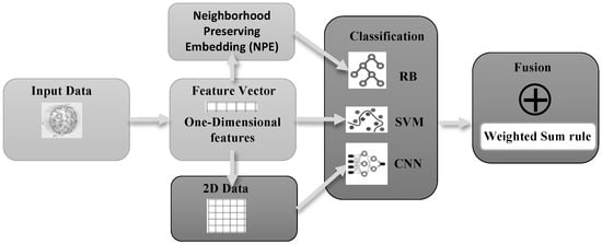
Figure 1.
Structure of the proposed approach: The input data is represented through a 1D vector that is used to train the SVMs. The same is also transformed with NPE to train RB. Specific transformations are applied to the 1D input in order to transform it into a 2D matrix to train the CNNs.
In the following sections, we give a brief description of all the methods adopted in this work, including those for comparison purposes.
3.1. Random Forest
The random forest algorithm [43] is based on decision trees and uses the bagging technique. This involves training multiple decision trees on different sections of the dataset by randomly selecting data points with replacements. Once trained, the model can predict the value of the target variable for new data based on the average of the predictions from the different trees. Random forest usually has better generalization performance than a single decision tree due to the randomness, which helps to reduce overfitting, thus decreasing the variance of the model. We used .
3.2. AdaBoost
The AdaBoost algorithm is a machine learning method that is employed to create regression or classification models [44]. It is a boosting technique that functions as an ensemble approach. During the training process, the algorithm focuses on those instances that have been misclassified. It assigns weights to each instance, with higher weights given to the incorrectly classified samples. We used 100 classifiers.
3.3. XGBoost
XGBoost is an improved version of gradient boosting, a technique developed by Friedman [45,46]. It uses a regularization term to prevent overfitting and thus achieve better results. Gradient boosting combines multiple models, such as random forest, to create a final model. It does this by giving more weight to instances with incorrect predictions. In each learning cycle, the prediction errors are used to calculate the gradient, and a new tree is created to predict the gradients. The prediction values are then updated. After the learning phase, XGBoost produces the final predictions of the target variable by adding the average calculated in the initial step to all the residuals predicted by the trees, multiplied by the learning rate. We used 100 classifiers.
3.4. Support Vector Machine (SVM)
SVM [47] is a classic binary classifier that works well in ensembles. For this reason, it was selected as the core classifier in several of our ensembles. SVM works by dividing an n-dimensional space (with n being the number of features) into two regions representing two distinct classes, referred to as the positive and negative classes. An n-dimensional hyperplane separates the two regions with the maximum distance d from the training vectors of the two classes. SVM is implemented using LibSVM, which is available at [48]. All the SVMs used in this work adopt the radial basis function. Moreover, a dataset-driven fine-tuning of parameters is performed on the SVMs by running a five-fold cross-validation using only the training data: i.e., if the testing protocol is a five-fold cross-validation, we run the five-fold for each of the five training sets. In this way, we try to avoid any overfitting. Hyperparameters are optimized by adopting a grid search approach with the following method (−5:2:15, −15:2:3).
3.5. Image Generator for Tabular Data (IGTD)
The objective of IGTD [36] is to convert tabular features into image features. Given two rank matrices R and Q of dimension , respectively, of tabular data and image, IGTD finds a mapping that minimizes the error:
where is a distance function (e.g., Euclidean distance), while and are the elements of R and Q. IGTD achieves the objective with an iterative process that swaps features of R until it converges or reaches a maximum number of iterations.
3.6. Random Subspace Rotation Boosting (RB)
RB is an ensemble of decision trees that randomly splits the features into subsets. RB corresponds to a random subspace version of rotating boosting [49]. In RB, subsets are changed by applying a feature transformation; for instance, in the original formulation of RB, features are reduced using PCA. As in [37], we apply NPE [50], which is designed to preserve the local manifold structure. In NPE, each data point is specified by a linear combination of the neighboring points, computed using KNN. The neighbors are represented as an adjacency matrix with weight from node i to node j computed as the minimum of . Then, the optimal embedding is such that the neighborhood structure can be preserved in the dimensionality-reduced space, given by the minimum eigenvalue solution:
where is the matrix of the points, , W is weight matrix with and .
3.7. Convolutional Neural Networks (CNNs)
In this work, we test four CNN topologies: ResNet18, ResNet50, ResNet101, and Inception ResNet v2. Many other topologies (VGG, DenseNet, GoogleNet, NasNet, DarkNet) were tested on the blood–brain barrier (BBB) dataset, but their performance was worse. Thus, they were not used to reduce test time. ResNet18, ResNet50, and ResNet101 are different versions of the ResNet architecture proposed in [51] and differ only in the depth of the networks. The main feature of ResNet is the presence of residual blocks. As shown in that figure, it is a standard convolutional block in a neural network, with the difference being that the input is summed to the output through a so-called residual connection. This trick helps gradient flow and mitigates the problem of vanishing and exploding gradients, allowing for better training. ResNet usually manages to reach a lower training error than older architectures with the same depth, thanks to the improved training.
Inception ResNet v2 [52] is the fusion between Inception v2 and ResNet. It is basically the Inception v2 architecture [53], with the difference that every inception module also has a residual connection.
The networks that we refer to here as stochastic [54] are modifications of CNN architectures whose activation functions have been randomly modified. Given a network and a pool of activation functions, we modify every activation layer of the original network with a new one randomly selected among those in the pool. This procedure yields a new network with a different activation. The randomness of the method yields a different network every time the algorithm is executed. The set of networks is then combined by the sum rule.
For feeding the CNNs, we reshape the original feature vector into a matrix. Given a feature vector , where is a single feature value, we want to obtain a matrix:
where and is the channel dimension while and are row and column coordinates. In order to obtain the matrix, we reshape the original feature vector f into a matrix by applying two different approaches.
In the first approach, each channel corresponds to the feature vector reshaped to match the column and row dimensions. The dimension of the matrix is . The value of are mapped into the first channel of the matrix as . For and the same procedure is repeated. If n is not a perfect square, then the feature vector is filled with zeros until is rational.
In the second approach, the feature vector is directly reshaped to match the matrix. The dimension of the matrix is since an image has three channels. The value of are mapped into with the following equation: . Similarly to the first approach, if is not a perfect square, then the feature vector is filled with zeros until is rational.
After the reshaping step, the resulting matrix is resized to match the input size requested by the specific CNN topology. Note that a random shuffling of the original features is performed to improve the diversity among the classifiers for each network in the ensemble before creating the matrices used to train the network.
3.8. Transformers in Image Classification
Deep learning has been dominated by CNN networks ever since their first appearance in 1989 [55], thanks to their structure, which is invariant to shift and less prone to overfitting. Their biggest impact has been in computer vision, where CNNs have become the mainstay for solving many tasks, such as image classification [51], semantic segmentation [56], and object detection [57]. While many researchers were developing more sophisticated CNN models, Vaswani et al. [58] was proposing the transformer to solve the machine translation problem. The transformer leverages self-attention mechanisms that have obtained disruptive performances in this area, thereby becoming the new leading paradigm in neural language processing.
Transformers were applied to image classification by Dosovitskiy et al. with a model named vision-transformer (ViT) [59], the first pure transformer model reaching results comparable to CNNs on image tasks. The authors adopted the encoder of the original transformer [58] by treating image patches as tokens. Training such a network is not effortless due to its lack of inductive biases. Moreover, aggregating local information is more difficult with the transformer model compared to standard CNNs [59,60]. To overcome these problems, ViT requires a pre-training on a dataset with millions of images, viz., the JFT-300M dataset [61].
A different approach to address the issue of data requirements was presented in [62]. The authors of that study proposed to distillate the knowledge from a CNN network combined with real ground-truth values. They also introduced a “distillation token” alongside the image tokens to improve the distillation process. These changes have simplified training and improved performance, resulting in a new model the authors called the data-efficient transformer (DeiT).
One of the best transformer models inspired by ViT is Swin [63]. It uses a hierarchical window structure that computes the self-attention inside a window, reducing execution time. Swin structure is also suitable for large-scale distributed training. The authors demonstrated that ViT can also be used as a backbone for other vision tasks, such as semantic segmentation [63].
Whereas ViT, DeiT, and Swin models may be considered “pure” transformer models, some authors have exploited the power of the CNN’s inductive bias and the transformer’s capacity within the same model. An example of this combination is CoAtNet [60], which merges depthwise convolution and self-attention, stacking them vertically to improve generalization, capacity, and efficiency.
Since training from random weights requires a huge amount of data, in this work, we fine-tune the models trained on ImageNet [64], available in the Timm library [65]. Specifically, we use DeiT-Base with patch dimension 16, ViT-Base with patch 16, Swin-Base with patch 4, and a specific implementation CoAtNet in Timm that removes the continuous log-coordinate relative position bias. It is worth mentioning that ViT implementation in Timm was first pretrained on Imagnet-21k. For each model, we changed the last layer to match the number of classes of the chosen dataset. In each dataset, we extracted a validation set with 0.25 split ratio to perform early-stopping to avoid overfitting, and we resized the dimension to 224 × 224 to match the input dimension of the pretrained networks.
We trained the models using AdamW optimizer with cosine annealing [66], starting from a learning rate of 10, weight decay value of 0.03, batch size of 32, and the standard cross-entropy loss. After five consecutive epochs without decreasing the minimum validation loss, we reduced the learning rate to 10 and 10. We kept the model with the best F1-score in the validation during the training.
With transformers, we created ensembles of them in the same way we create ensembles for CNNs.
4. Experimental Results
To assess the proposed approach, we performed an empirical evaluation using the following medical datasets (along with a large dataset based on stars that will be used in one of our experiments):
- RNA: This is the tumor gene expression dataset published in [67]. It contains the RNA sequencing values from tumor samples belonging to five cancer types: (a) lung squamous cell carcinoma (LUSC), (b) lung adenocarcinoma (LUAD), (c) breast invasive carcinoma (BRCA), (d) uterine corpus endometrial carcinoma (UCEC), and (e) kidney renal clear-cell carcinoma (KIRC). This dataset contains 2086 patterns with 972 features. The number of samples for each tumor is reported in Table 1. The protocol for RNA is five-fold cross-validation.
 Table 1. Number of samples for tumor category in RNA dataset.
 - Two datasets that predict blood–brain barrier (BBB) permeability of compounds:
- BBB: This dataset contains 7162 compounds [68] with 5453 BBB-permeable and 1709 non-permeable compounds. The protocol for BBB is 10-fold cross-validation.
- BBBind: This dataset contains 74 central nerve system compounds gathered from the literature, with 39 BBB compounds permeable and 35 nonpermeable. The 74 compounds are classified with models trained on the first BBB dataset of 7162 compounds.
- Enz: This is the drug–enzyme interaction dataset in [69]. Enz is composed of 445 drugs, 664 targets, and 2926 interactions. The drug molecules are encoded by a substructure fingerprint with a dictionary of substructure patterns. The discrete wavelet transform (DWT) is applied simultaneously to extract features from the target sequences, after which the feature vectors are constructed by concatenating and normalizing the target, drug, and network. The protocol for Enz is five-fold cross-validation.
- Two datasets for prognosis prediction of breast cancer [70]. The dataset consists of data from 1980 patients. Patients were classified as long-time survivors (greater than five years), of which there are 1489 patients, and short-term survivors (less than five years), of which there are 491. The two datasets, labeled as follows, differ in the features that represent each patient:
- Breast, wherein the features are the gene expression profile, copy number alteration (CNA) profile, and clinical data, as suggested in [70].
- Breast_L, where a CNN is used for feature extraction, as in [70].
The protocol for both breast cancer datasets is five-fold cross-validation. - InSilico: It is a drug repositioning dataset [71]; the goal of this application is to find new uses for existing drugs (the dataset is originally called Fdataset). In the dataset, there are 1933 associations between drugs and diseases, 593 drugs, and 313 diseases. Interacting drug–disease pairs are used as positive samples, and the same number of pairs with no known interactions are randomly selected as negative samples. Finally, 10-fold cross-validation is used to evaluate performance. In this work, we employ the same feature extraction applied originally. Features are [0, 1], if we do not normalize, and [0, 255] otherwise. CNN networks do not converge well, and poor performance is obtained when features are not normalized. Hence, all tests reported for CNN use features normalized to [0, 255], which is obtained by simply multiplying each unnormalized feature by 255.
- Pestis: This dataset corresponds to the original Human–Yersinia pestis datasets, and contains features for understanding the behavioral process of life and disease-causing mechanism in terms of protein–protein interactions (PPI) [72]. In the interaction dataset, the numbers of positive and negative interactions are 4097 and 12,500, respectively. The protocol for Pestis is five-fold cross-validation.
- Kepler: This is not a medical dataset. We use the same threshold crossing event (TCE) catalog, from the Kepler data in [73]. A TCE is a sequence of significant, periodic, planet-transit-like features in the light curve of a target star. This TCE catalog contains a total of 18,407 TCEs, and each TCE is described by 237 attributes that are based on, e.g., the wavelet matched filter, transit model fitting, and difference image centroids. The aim is to assign to each TCE one of these four classes: planet candidate; astrophysical false positive; non-transiting phenomena; and unknown object. To reduce computation time, we run a two-fold cross-validation
- Alz: Data were obtained from the Alzheimer’s Disease Neuroimaging Initiative (ADNI) database (adni.loni.usc.edu); it has been collected from 41 different radiology centers. The aim is to classify the mildly cognitive impaired converting to Alzheimer’s Disease (MCIc) vs. cognitively normal (CN) subjects. We apply the same testing protocol (20-fold cross-validation), preprocessing, and the number of features of [74]. We have 162 CN and 76 MCIc patterns, each described by 2000 features selected by the Chi-2 test feature selection approach.
For all datasets with k-fold cross-validation, the split is performed five times, and performance reports the average values. For training and testing the SVMs, the features are normalized to [0, 1] using only the data in the training set. Two metrics are adopted as the performance indicators: error rate and the error area under the ROC curve (EAUC).
We report the performance obtained in the following experiments using different CNN topologies. The following models were considered:
- Base: a single CNN;
- Ens: an ensemble obtained with 14 reiterated CNNs, where all of them use ReLu as the activation function;
- Stoc: an ensemble of 14 CNNs obtained using the stochastic approach detailed in the previous section.
Stoc is built with fourteen classifiers, seven using the first method reported in Section 3.7 and seven with the approach reported in Section 3.7 for reshaping a vector to a matrix. ResNet50 (DeepIns) is ResNet50 coupled with the method proposed in [11] for feeding CNNs using matrices built starting from the standard feature vector. In this case, Stoc is always coupled with the matrices created by DeepIns. The size of Ens and Stoc is always 14, even when IGTD is coupled with the 14 CNNs trained using the stochastic approach. Moreover, in each ensemble (including DeepIns and IGTD), each CNN is trained randomly by shuffling the features before reshaping the feature vector into a matrix to increase diversity among ensemble elements. The networks are combined by the weighted sum rule (the weight is 1 if unspecified). Specifically, we investigated the following:
- ResNet18 + ResNet50 + ResNet101, which adopts the sum rule between ResNet18, ResNet50, and ResNet101, each coupled with Stoc.
- ResNet18 + ResNet50 + ResNet101 (IGTD), which adopts the sum rule between ResNet18, ResNet50, and ResNet101. Each model is coupled with Stoc, where the IGTD approach has been used for creating the matrices used to feed the CNNs.
- ReShape + IGTD, which adopts the sum rule between ResNet18 + ResNet50 + ResNet101 and ResNet18 + ResNet50 + ResNet101 (IGTD).
The first set of experiments is reported in Table 2 and Table 3. Examining the results in those tables, we observe that the best tradeoff between performance and computational complexity is obtained on average by ResNet50. We also note that our approach is more stable in performance than DeepIns. Moreover, both the Stoc and Ens ensembles outperform the Base approach. As always happens with CNNs, the computational complexity is essentially related to training and not to the inference phase. Using an NVIDIA 1080, the time it takes to classify 100 patterns in the following are:
Table 2.
CNN error rate; to reduce computation time some tests are not performed. Best performance in bold.
Table 3.
CNN error area under the ROC curve; to reduce computation time some tests are not performed. Best performance in bold.
- Resnet50 takes 0.30 s;
- ResNet101 takes 0.35 s;
- ResNet18 takes 0.16 s.
Note: the input for ResNet above is always the same since they are pretrained on ImageNet.
Table 4.
Proposed ensemble and error rate. Best performance in bold.
Table 5.
Proposed ensemble and error area under the ROC curve. Best performance in bold.
- SVM: where the parameters are found separately in each training set of each fold using a grid search;
- RB: where a random subspace of 10 RBs are combined by sum rule;
- Deep: ResNet50 coupled with Stoc;
- DeepIG: the method previously defined as ReShape+IGTD;
- “k × SVM + RB + Deep/DeepIG”: an ensemble that is the weighted sum rule among SVM (weight = k), RB, and Deep/DeepIG (the scores of each approach, i.e., Deep, SVM, RB, and DeepIG, are normalized to mean 0 and std 1 before the fusion).
- State of the art: this corresponds to the best method reported on that dataset: [69] for Enz, [68] for BBB and BBB-Ind, [67] for RNA, [70] for Breast and Breast_L, and [71] for InSilico.
- There is no clear winner among SVM, RB, and Deep;
- Deep performs better than the transformers;
- On average, the best method, considering all the datasets and both the performance indicators, is 4 × SVM + RB + DeepIG; this ensemble obtains similar or better performance compared to the state of the art in all the datasets and is our suggested ensemble.
From the results in Table 4 and Table 5, it can be seen that the ensemble 4 × SVM + RB + Deep is similar to or better than SVM. The latter is still used by many as a basic classification method when working with feature vectors. It is unclear whether CNN-1d can replace SVM, but we envision that by providing the code, many could benefit from our solution and use ’4 × SVM + RB + Deep’/’4 × SVM + RB + DeepIG’ instead of SVM. Considering the results reported in Table 5, “4 × SVM + RB+ DeepIG” outperforms SVM with a p-value of 0.0312, using the Wilcoxon signed-rank test. Keep in mind that we are adopting SVM by LibSVM (https://github.com/cjlin1/libsvm—Last access, 13 March 2023), by far the most used SVM tool, and we also fix SVM weights following a five-fold cross-validation on each training set as best practice. This procedure should be widely adopted, but in the literature, some approaches still use the entire dataset to set weights, thereby overfitting. Note as well that despite some research already proposed in the literature on using ensembles, none supplants SVM. Thus, our main novelty here is the successful combination of SVM with CNN using classic image-based topologies.
We tested many different networks, but only ResNet-based networks performed similarly to SVM and RB. Moreover, DeepIns seems to be unstable as it works poorly in some datasets; notice that we are using the original tool.
For each test, we also evaluate and compare the ability to perform a classification task. To do that, we adopt the receiver operator characteristic (ROC) curve. An ROC curve is a graphical representation used to show the diagnostic capabilities of binary classification. The ROC curve is built by plotting the true positive rate (TPR) versus the false positive rate (FPR). TPR represents the percentage of all positive observations that are correctly predicted to be positive. Similarly, FPR depicts the percentage of falsely predicted positive observations out of all negative observations. The ROC curve shows the trade-off between sensitivity (or TPR) and specificity (1—FPR). The closer the yield curve is to the upper left corner, the better the performance is. Any random classification produces a plot around the diagonal (FPR = TPR). The ROC curve is indifferent to class imbalance. Here, we report the ROC curves of tests where our approach performs better than SVM. In other cases, performances are mostly overlapping. In Figure 2, we compare the ROC curves for our proposed ensemble (red line in the figure) and SVM (blue line in the figure). In each ROC curve, it can be noticed that the proposed ensemble is always performing better than the standard SVM (as in the many points where the red line is above the blue line). This is evidence that suggests that the proposed methods are outperforming the standard SVM classifier.
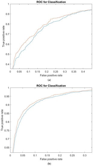
Figure 2.
ROC curves for different datasets: (a) BREAST dataset; (b) Pestis dataset. Ensemble (red line) and SVM (blue line).
In addition to the tests above, we also evaluated our approach on two other large datasets (Kepler and Pestis) and a small one (Alz). Due to computational power resource limitations, on these datasets, we ran only a subset of the previous experiments. Table 6, Table 7 and Table 8 report the performance of our proposal and the results of recent literature on the above-cited datasets. As can be observed, in the very small dataset (200 patterns), CNN, as expected, suffers; the other two datasets contain thousands of patterns and confirm that the proposed ensemble improves the stand-alone SVM. We are aware that in [75] better performance is obtained in Pestis, but we were not able to reproduce the same results adopting our testing protocol.
Table 6.
Performance on Pestis dataset. Best performance in bold.
Table 7.
Performance on Alzheimer dataset. Best performance in bold.
Table 8.
Performance on Kepler dataset. Best performance in bold.
As a final test, we attempted to improve the performance of the ensemble by using a validation set to find the weights of the three methods (SVM, RB, and DeepIG) that make up the ensemble. As an approach for extracting the validation set, we used five-fold cross-validation only on the data from the training set. The results do not allow us to come to a definitive conclusion: in some datasets, the use of validation improves performance; in others, it does not (probably as a consequence of overfitting the parameters on the validation set). The results are reported in Table 9, where A, B, and C are the weights obtained using the validation data. Although in the ALZ dataset the proposed method performs worse than SVM, the importance of the ensemble is evident: the EAUC of a single ResNet50 coupled to Deep is 19.03, the EAUC of a single ResNet50 coupled to IGTD is 18.62, while the EAUC of the DeepIG ensemble is 13.95. Even in the Kepler dataset, the importance of the ensemble is evident, as the EAUC of a single ResNet50 coupled with Deep is 7.56, the EAUC of a single ResNet50 coupled with IGTD is 9.03, and the EAUC of the DeepIG ensemble is 4.48. In contrast, for the Pestis dataset, we obtain the following performance: the EAUC of a single ResNet50 coupled with Deep is 4.59, the EAUC of a single ResNet50 coupled with IGTD is 3.68, while the EAUC of the DeepIG ensemble is 2.65.
Table 9.
Proposed ensemble validation set: EAUC.
5. Conclusions
In this work, we investigated training CNNs with matrices generated by reshaping original feature vectors. We also reported the performance obtained by combining CNN and vector-based descriptors. The research presented here sheds more light on this area by exploring different topologies and the value of combining different classifiers to build heterogeneous ensembles. From this analysis, we found that approaches based on ResNet performed the best. Our approach has been tested on several different datasets to check generalizability. Across the board, we obtained results that were close to or better than the state of the art.
In future works, we plan to add new datasets to improve the analysis of the generalization of our method as well as test other methods (also proposed in the literature) to create a suitable matrix to train CNN. Other future lines of research will be:
- Data normalization: it is important to understand the best way to pass data to pre-trained networks on images;
- Adapting methods based on the dataset: e.g., if we know that the input consists of a sequence of only four letters (as with DNA or RNA), we can adapt the methods to create ad hoc ones considering that we know what possible features are present;
- Working towards achieving a more contextual transformation method related to data semantics.
Finally, note that in the proposed framework, we used a CNN pretrained on ImageNet. The next step will analyze the performance of pretraining other datasets, e.g., by adopting more datasets and then adopting a leave-one-out approach where one dataset is used for testing and the other datasets are used to pretrain the model. We are planning new methods to transform vectors in matrices in order to maintain as much information as possible avoiding biases. We strongly believe that reported results may also prompt other authors to work on the same task of adapting classic CNNs to be used to classify feature vectors.
Author Contributions
Conceptualization, L.N.; software, L.N. and L.B.; writing—original draft preparation, A.L., S.B. and L.N.; writing—review and editing, A.L., S.B. and L.N. All authors have read and agreed to the published version of the manuscript.
Funding
This research received no external funding.
Institutional Review Board Statement
Not applicable.
Informed Consent Statement
Not applicable.
Data Availability Statement
All the code required to replicate our experiments is available at https://github.com/LorisNanni.
Acknowledgments
We would like to acknowledge the support that NVIDIA provided us through the GPU Grant Program. We used a donated TitanX GPU to train the neural networks discussed in this work.
Conflicts of Interest
The authors declare no conflict of interest.
References
- Poggio, T. Image representations for visual learning. Lect. Notes Comput. Sci. (Incl. Subser. Lect. Notes Artif. Intell. Lect. Notes Bioinform.) 1997, 1206, 143. [Google Scholar] [CrossRef]
- Zhu, L.; Hu, Q.; Yang, J.; Zhang, J.; Xu, P.; Ying, N. EEG signal classification using manifold learning and matrix-variate Gaussian model. Comput. Intell. Neurosci. 2021, 2021, 6668859. [Google Scholar] [CrossRef]
- Nanni, L.; Brahnam, S.; Lumini, A. Ensemble of Deep Learning Approaches for ATC Classification. In Smart Innovation, Systems and Technologies; Springer: Singapore, 2020; Volume 159, pp. 117–125. [Google Scholar] [CrossRef]
- Loreggia, A.; Malitsky, Y.; Samulowitz, H.; Saraswat, V. Deep learning for algorithm portfolios. In Proceedings of the AAAI Conference on Artificial Intelligence, Phoenix, AR, USA, 12–17 February 2016; Volume 30. [Google Scholar]
- Yoshimori, A. Prediction of molecular properties using molecular topographic map. Molecules 2021, 26, 4475. [Google Scholar] [CrossRef] [PubMed]
- Akbari Rokn Abadi, S.; Mohammadi, A.; Koohi, S. WalkIm: Compact image-based encoding for high-performance classification of biological sequences using simple tuning-free CNNs. PLoS ONE 2022, 17, e0267106. [Google Scholar] [CrossRef] [PubMed]
- Wang, H.; Li, G.; Wang, Z. Fast SVM classifier for large-scale classification problems. Inf. Sci. 2023, 642, 119136. [Google Scholar] [CrossRef]
- Shao, Y.H.; Lv, X.J.; Huang, L.W.; Bai, L. Twin SVM for conditional probability estimation in binary and multiclass classification. Pattern Recognit. 2023, 136, 109253. [Google Scholar] [CrossRef]
- Bania, R.K.; Halder, A. R-HEFS: Rough set based heterogeneous ensemble feature selection method for medical data classification. Artif. Intell. Med. 2021, 114, 102049. [Google Scholar] [CrossRef]
- Teimouri, H.; Medvedeva, A.; Kolomeisky, A.B. Bacteria-Specific Feature Selection for Enhanced Antimicrobial Peptide Activity Predictions Using Machine-Learning Methods. J. Chem. Inf. Model. 2023, 63, 1723–1733. [Google Scholar] [CrossRef]
- Sharma, A.; Vans, E.; Shigemizu, D.; Boroevich, K.A.; Tsunoda, T. DeepInsight: A methodology to transform a non-image data to an image for convolution neural network architecture. Sci. Rep. 2019, 9, 11399. [Google Scholar] [CrossRef]
- Gokhale, M.; Mohanty, S.K.; Ojha, A. GeneViT: Gene Vision Transformer with Improved DeepInsight for cancer classification. Comput. Biol. Med. 2023, 155, 106643. [Google Scholar] [CrossRef]
- Yang, J.; Zhang, D.; Frangi, A.F.; Yang, J.Y. Two-Dimensional PCA: A New Approach to Appearance-Based Face Representation and Recognition. IEEE Trans. Pattern Anal. Mach. Intell. 2004, 26, 131–137. [Google Scholar] [CrossRef] [PubMed]
- Li, J.; Janardan, R.; Li, Q. Two-dimensional linear discriminant analysis. Adv. Neural Inf. Process. Syst. 2002, 17, 1569–1576. [Google Scholar]
- Zheng, W.S.; Lai, J.H.; Li, S.Z. 1D-LDA vs. 2D-LDA: When is vector-based linear discriminant analysis better than matrix-based? Pattern Recognit. 2008, 41, 2156–2172. [Google Scholar] [CrossRef]
- Zhi, R.; Ruan, Q. Facial expression recognition based on two-dimensional discriminant locality preserving projections. Neurocomputing 2008, 71, 1730–1734. [Google Scholar] [CrossRef]
- Razzak, I.; Saris, R.A.; Blumenstein, M.; Xu, G. Integrating joint feature selection into subspace learning: A formulation of 2DPCA for outliers robust feature selection. Neural Netw. 2020, 121, 441–451. [Google Scholar] [CrossRef] [PubMed]
- Hancherngchai, K.; Titijaroonroj, T.; Rungrattanaubol, J. An individual local mean-based 2DPCA for face recognition under illumination effects. In Proceedings of the 2019 16th International Joint Conference on Computer Science and Software Engineering (JCSSE), Chonburi, Thailand, 10–12 July 2019; pp. 213–217. [Google Scholar]
- Titijaroonroj, T.; Hancherngchai, K.; Rungrattanaubol, J. Regional covariance matrix-based two-dimensional pca for face recognition. In Proceedings of the 2020 12th International Conference on Knowledge and Smart Technology (KST), Markham, ON, Canada, 10–13 November 2020; pp. 6–11. [Google Scholar]
- Pal, R.; Saraswat, M. A new weighted two-dimensional vector quantisation encoding method in bag-of-features for histopathological image classification. Int. J. Intell. Inf. Database Syst. 2020, 13, 150–171. [Google Scholar] [CrossRef]
- Zhao, M.X.; Jia, Z.G.; Gong, D.W.; Zhang, Y. Data-Driven Bilateral Generalized Two-Dimensional Quaternion Principal Component Analysis with Application to Color Face Recognition. arXiv 2023, arXiv:2306.07045. [Google Scholar]
- Eustice, R.; Pizarro, O.; Singh, H.; Howland, J. UWIE underwater image toolbox for optical image processing and mosaicking in MATLAB. In Proceedings of the Underwater Technology, Tokyo, Japan, 19 April 2002; Volume 2002, pp. 141–145. [Google Scholar] [CrossRef]
- Brahnam, S.; Jain, L.C.; Lumini, A.; Nanni, L. Introduction to Local Binary Patterns: New Variants and Applications; Springer: Berlin, Germany, 2014; Volume 506, pp. 1–13. [Google Scholar] [CrossRef]
- Uddin, J.; Islam, R.; Kim, J.M.; Kim, C.H. A Two-Dimensional Fault Diagnosis Model of Induction Motors using a Gabor Filter on Segmented Images. Int. J. Control. Autom. 2016, 9, 11–22. [Google Scholar] [CrossRef]
- Chen, S.; Zhu, Y.; Zhang, D.; Yang, J.Y. Feature extraction approaches based on matrix pattern: MatPCA and MatFLDA. Pattern Recognit. Lett. 2005, 26, 1157–1167. [Google Scholar] [CrossRef]
- Wang, Z.; Chen, S. Matrix-pattern-oriented least squares support vector classifier with AdaBoost. Pattern Recognit. Lett. 2008, 29, 745–753. [Google Scholar] [CrossRef]
- Liu, J.; Chen, S. Non-iterative generalized low rank approximation of matrices. Pattern Recognit. Lett. 2006, 27, 1002–1008. [Google Scholar] [CrossRef]
- Wang, Z.; Chen, S.; Liu, J.; Zhang, D. Pattern representation in feature extraction and classifier design: Matrix versus vector. IEEE Trans. Neural Netw. 2008, 19, 758–769. [Google Scholar] [CrossRef] [PubMed]
- Kim, C.; Choi, C.H. A discriminant analysis using composite features for classification problems. Pattern Recognit. 2007, 40, 2958–2966. [Google Scholar] [CrossRef]
- Nanni, L.; Brahnam, S.; Lumini, A. Local Ternary Patterns from Three Orthogonal Planes for human action classification. Expert Syst. Appl. 2011, 38, 5125–5128. [Google Scholar] [CrossRef]
- Felzenszwalb, P.F.; McAuley, J.J. Fast inference with min-sum matrix product. IEEE Trans. Pattern Anal. Mach. Intell. 2011, 33, 2549–2554. [Google Scholar] [CrossRef] [PubMed]
- Lee, D.D.; Seung, H.S. Algorithms for non-negative matrix factorization. Adv. Neural Inf. Process. Syst. 2001, 13, 556–562. [Google Scholar]
- Chen, S.; Wang, Z.; Tian, Y. Matrix-pattern-oriented Ho-Kashyap classifier with regularization learning. Pattern Recognit. 2007, 40, 1533–1543. [Google Scholar] [CrossRef]
- Song, F.; Guo, Z.; Chen, Q. Two-dimensional nearest neighbor classifiers for face recognition. In Proceedings of the 2012 International Conference on Systems and Informatics, ICSAI 2012, Yantai, China, 19–20 May 2012; pp. 2682–2686. [Google Scholar] [CrossRef]
- Shen, W.X.; Zeng, X.; Zhu, F.; Wang, Y.L.; Qin, C.; Tan, Y.; Jiang, Y.Y.; Chen, Y.Z. Out-of-the-box deep learning prediction of pharmaceutical properties by broadly learned knowledge-based molecular representations. Nat. Mach. Intell. 2021, 3, 334–343. [Google Scholar] [CrossRef]
- Zhu, Y.; Brettin, T.; Xia, F.; Partin, A.; Shukla, M.; Yoo, H.; Evrard, Y.A.; Doroshow, J.H.; Stevens, R.L. Converting tabular data into images for deep learning with convolutional neural networks. Sci. Rep. 2021, 11, 11325. [Google Scholar] [CrossRef]
- Nanni, L.; Brahnam, S.; Ghidoni, S.; Lumini, A. Toward a General-Purpose Heterogeneous Ensemble for Pattern Classification. Comput. Intell. Neurosci. 2015, 2015, 1–10. [Google Scholar] [CrossRef]
- Kotsiantis, S.; Tampakas, V. Combining heterogeneous classifiers: A recent overview. J. Converg. Inf. Technol. 2011, 6, 164–172. [Google Scholar] [CrossRef]
- Melville, P.; Mooney, R.J. Creating diversity in ensembles using artificial data. Inf. Fusion 2005, 6, 99–111. [Google Scholar] [CrossRef]
- Pang, T.; Xu, K.; Du, C.; Chen, N.; Zhu, J. Improving adversarial robustness via promoting ensemble diversity. In Proceedings of the 36th International Conference on Machine Learning, ICML 2019, Long Beach, CA, USA, 9–15 June 2019; Volume 2019, pp. 8759–8771. [Google Scholar]
- Amelio, A.; Bonifazi, G.; Corradini, E.; Di Saverio, S.; Marchetti, M.; Ursino, D.; Virgili, L. Defining a deep neural network ensemble for identifying fabric colors. Appl. Soft Comput. 2022, 130, 109687. [Google Scholar] [CrossRef]
- Cornelio, C.; Donini, M.; Loreggia, A.; Pini, M.S.; Rossi, F. Voting with random classifiers (VORACE): Theoretical and experimental analysis. Auton. Agents -Multi-Agent Syst. 2021, 35, 22. [Google Scholar] [CrossRef]
- Breiman, L. Random forests. Mach. Learn. 2001, 45, 5–32. [Google Scholar] [CrossRef]
- Schapire, R.E. Explaining adaboost. In Empirical Inference; Springer: Berlin/Heidelberg, Germany, 2013; pp. 37–52. [Google Scholar]
- Friedman, J.H. Stochastic gradient boosting. Comput. Stat. Data Anal. 2002, 38, 367–378. [Google Scholar] [CrossRef]
- Friedman, J.H. Greedy function approximation: A gradient boosting machine. Ann. Stat. 2001, 29, 1189–1232. [Google Scholar] [CrossRef]
- Andrew, A.M. An Introduction to Support Vector Machines and Other Kernel-Based Learning Methods; Cambridge University Press: Cambridge, UK, 2001; Volume 30, pp. 103–115. [Google Scholar] [CrossRef]
- Chang, C.C.; Lin, C.J. LIBSVM: A Library for Support Vector Machines. Acm Trans. Intell. Syst. Technol. (TIST) 2011, 2, 1–39. [Google Scholar] [CrossRef]
- Zhang, C.X.; Zhang, J.S. RotBoost: A technique for combining Rotation Forest and AdaBoost. Pattern Recognit. Lett. 2008, 29, 1524–1536. [Google Scholar] [CrossRef]
- He, X.; Cai, D.; Yan, S.; Zhang, H.J. Neighborhood preserving embedding. In Proceedings of the Tenth IEEE International Conference on Computer Vision (ICCV’05) Volume 1, Beijing, China, 17–21 October 2005; Volume 2, pp. 1208–1213. [Google Scholar]
- He, K.; Zhang, X.; Ren, S.; Sun, J. Deep residual learning for image recognition. In Proceedings of the IEEE Computer Society Conference on Computer Vision and Pattern Recognition, Las Vegas, NV, USA, 26 June–1 July 2016; Volume 2016, pp. 770–778. [CrossRef]
- Szegedy, C.; Ioffe, S.; Vanhoucke, V.; Alemi, A.A. Inception-V4, Inception-Resnet and the Impact of Residual Connections on Learning; Cornell University: Ithaca, NY, USA, 2017; pp. 4278–4284. [Google Scholar] [CrossRef]
- Ioffe, S.; Szegedy, C. Batch normalization: Accelerating deep network training by reducing internal covariate shift. In Proceedings of the 32nd International Conference on Machine Learning, ICML 2015, Lille, France, 6–11 July 2015; Volume 1, pp. 448–456. [Google Scholar]
- Nanni, L.; Lumini, A.; Ghidoni, S.; Maguolo, G. Stochastic selection of activation layers for convolutional neural networks. Sensors 2020, 20, 1626. [Google Scholar] [CrossRef]
- LeCun, Y.; Boser, B.; Denker, J.; Henderson, D.; Howard, R.; Hubbard, W.; Jackel, L. Handwritten digit recognition with a back-propagation network. Adv. Neural Inf. Process. Syst. 1989, 2, 396–404. [Google Scholar]
- Chen, L.C.; Papandreou, G.; Kokkinos, I.; Murphy, K.; Yuille, A.L. Deeplab: Semantic image segmentation with deep convolutional nets, atrous convolution, and fully connected crfs. IEEE Trans. Pattern Anal. Mach. Intell. 2017, 40, 834–848. [Google Scholar] [CrossRef] [PubMed]
- Girshick, R. Fast r-cnn. In Proceedings of the IEEE International Conference on Computer Vision, Santiago, Chile, 7–13 December 2015; pp. 1440–1448. [Google Scholar]
- Vaswani, A.; Shazeer, N.; Parmar, N.; Uszkoreit, J.; Jones, L.; Gomez, A.N.; Kaiser, Ł.; Polosukhin, I. Attention is all you need. Adv. Neural Inf. Process. Syst. 2017, 30, 5998–6008. [Google Scholar]
- Dosovitskiy, A.; Beyer, L.; Kolesnikov, A.; Weissenborn, D.; Zhai, X.; Unterthiner, T.; Dehghani, M.; Minderer, M.; Heigold, G.; Gelly, S.; et al. An image is worth 16x16 words: Transformers for image recognition at scale. arXiv 2020, arXiv:2010.11929. [Google Scholar]
- Dai, Z.; Liu, H.; Le, Q.V.; Tan, M. Coatnet: Marrying convolution and attention for all data sizes. Adv. Neural Inf. Process. Syst. 2021, 34, 3965–3977. [Google Scholar]
- Sun, C.; Shrivastava, A.; Singh, S.; Gupta, A. Revisiting unreasonable effectiveness of data in deep learning era. In Proceedings of the IEEE International Conference on Computer Vision, Venice, Italy, 22–29 October 2017; pp. 843–852. [Google Scholar]
- Touvron, H.; Cord, M.; Douze, M.; Massa, F.; Sablayrolles, A.; Jégou, H. Training data-efficient image transformers & distillation through attention. In Proceedings of the International Conference on Machine Learning, PMLR, Virtual, 18–24 July 2021; pp. 10347–10357. [Google Scholar]
- Liu, Z.; Lin, Y.; Cao, Y.; Hu, H.; Wei, Y.; Zhang, Z.; Lin, S.; Guo, B. Swin transformer: Hierarchical vision transformer using shifted windows. In Proceedings of the IEEE/CVF International Conference on Computer Vision, Virtual, 11–17 October 2021; pp. 10012–10022. [Google Scholar]
- Krizhevsky, A.; Sutskever, I.; Hinton, G.E. Imagenet classification with deep convolutional neural networks. Commun. ACM 2017, 60, 84–90. [Google Scholar] [CrossRef]
- Wightman, R. PyTorch Image Models. 2019. Available online: https://github.com/rwightman/pytorch-image-models (accessed on 3 August 2023). [CrossRef]
- Loshchilov, I.; Hutter, F. Fixing weight decay regularization in adam. In Proceedings of the ICLR 2018 Conference Blind Submission, Vancouver, BC, Canada, 30 April–3 May 2017. [Google Scholar]
- Khalifa, N.E.M.; Taha, M.H.N.; Ezzat Ali, D.; Slowik, A.; Hassanien, A.E. Artificial intelligence technique for gene expression by tumor RNA-Seq Data: A novel optimized deep learning approach. IEEE Access 2020, 8, 22874–22883. [Google Scholar] [CrossRef]
- Shaker, B.; Yu, M.S.; Song, J.S.; Ahn, S.; Ryu, J.Y.; Oh, K.S.; Na, D. LightBBB: Computational prediction model of blood-brain-barrier penetration based on LightGBM. Bioinformatics 2021, 37, 1135–1139. [Google Scholar] [CrossRef]
- Shen, C.; Ding, Y.; Tang, J.; Xu, X.; Guo, F. An ameliorated prediction of drug–target interactions based on multi-scale discretewavelet transform and network features. Int. J. Mol. Sci. 2017, 18, 1781. [Google Scholar] [CrossRef]
- Arya, N.; Saha, S. Multi-Modal Classification for Human Breast Cancer Prognosis Prediction: Proposal of Deep-Learning Based Stacked Ensemble Model. IEEE/ACM Trans. Comput. Biol. Bioinform. 2022, 19, 1032–1041. [Google Scholar] [CrossRef]
- Yi, H.C.; You, Z.H.; Wang, L.; Su, X.R.; Zhou, X.; Jiang, T.H. In silico drug repositioning using deep learning and comprehensive similarity measures. BMC Bioinform. 2021, 22, 293. [Google Scholar] [CrossRef]
- Kösesoy, İ.; Gök, M.; Öz, C. A new sequence based encoding for prediction of host–pathogen protein interactions. Comput. Biol. Chem. 2019, 78, 170–177. [Google Scholar] [CrossRef]
- McCauliff, S.D.; Jenkins, J.M.; Catanzarite, J.; Burke, C.J.; Coughlin, J.L.; Twicken, J.D.; Tenenbaum, P.; Seader, S.; Li, J.; Cote, M. Automatic Classification of Kepler Planetary Transit Candidates. Astrophys. J. 2015, 806, 6. [Google Scholar] [CrossRef]
- Nanni, L.; Interlenghi, M.; Brahnam, S.; Salvatore, C.; Papa, S.; Nemni, R.; Castiglioni, I.; the Alzheimer’s Disease Neuroimaging Initiative. Comparison of Transfer Learning and Conventional Machine Learning Applied to Structural Brain MRI for the Early Diagnosis and Prognosis of Alzheimer’s Disease. Front. Neurol. 2020, 11, 576194. [Google Scholar] [CrossRef] [PubMed]
- Mahapatra, S.; Gupta, V.R.; Sahu, S.S.; Panda, G. Deep neural network and extreme gradient boosting based Hybrid classifier for improved prediction of Protein-Protein interaction. IEEE/ACM Trans. Comput. Biol. Bioinform. 2021, 19, 155–165. [Google Scholar] [CrossRef]
- Mahapatra, S.; Sahu, S.S. Boosting predictions of Host-Pathogen protein interactions using Deep neural networks. In Proceedings of the 2020 IEEE International Students’ Conference on Electrical, Electronics and Computer Science (SCEECS), Bhopal, India, 22–23 February 2020; pp. 1–4. [Google Scholar]
- Li, X.; Han, P.; Wang, G.; Chen, W.; Wang, S.; Song, T. SDNN-PPI: Self-attention with deep neural network effect on protein-protein interaction prediction. BMC Genom. 2022, 23, 474. [Google Scholar] [CrossRef] [PubMed]
Disclaimer/Publisher’s Note: The statements, opinions and data contained in all publications are solely those of the individual author(s) and contributor(s) and not of MDPI and/or the editor(s). MDPI and/or the editor(s) disclaim responsibility for any injury to people or property resulting from any ideas, methods, instructions or products referred to in the content. |
© 2023 by the authors. Licensee MDPI, Basel, Switzerland. This article is an open access article distributed under the terms and conditions of the Creative Commons Attribution (CC BY) license (https://creativecommons.org/licenses/by/4.0/).