Optimal Matching with Matching Priority

Abstract

Matching algorithms are commonly used to build comparable subsets (matchings) in observational studies. When a complete matching is not possible, some units must necessarily be excluded from the final matching. This may bias the final estimates comparing the two populations, and thus it is important to reduce the number of drops to avoid unsatisfactory results. Greedy matching algorithms may not reach the maximum matching size, thus dropping more units than necessary. Optimal matching algorithms do ensure a maximum matching size, but they implicitly assume that all units have the same matching priority. In this paper, we propose a matching strategy which is order optimal in the sense that it finds a maximum matching size which is consistent with a given matching priority. The strategy is based on an order-optimal matching algorithm originally proposed in connection with assignment problems by D. Gale. When a matching priority is given, the algorithm ensures that the discarded units have the lowest possible matching priority. We discuss the algorithm’s complexity and its relation with classic optimal matching. We illustrate its use with a problem in a case study concerning a comparison of female and male executives and a simulation.

1. Introduction

Matching algorithms are an established method for balancing covariates across two samples of units, usually treated and control units. A matching algorithm is designed to find a matched subset of the original data where the covariate balance across the treated and control units is similar to that arising from a randomized experiment. Under a set of hypothesis known as Rubin’s causal framework [1], a balanced matched subset makes possible drawing causal inferences from observational data. Given the cost and difficulties of randomized experiments, in contrast with the increasingly large availability of observational data, matching has become a standard tool for research in comparative studies [2]. The researcher first chooses a suitable cost function for measuring the dissimilarity between the covariates of treated and control units (possibly specifying a maximum matching cost (i.e., the caliper) and then selects a matching algorithm in order to obtain comparable subsets of treated and control units (the final matching).

Classic matching algorithms are designed to build matched pairs of treated and control units. In their simplest form of nearest neighbor 1:1 matching, each treated unit is sequentially matched with the control at minimum dissimilarity. These algorithms are sometimes referred to as “greedy” because they match units sequentially, so that the dissimilarity is minimized only “locally”, without considering the whole matching cost. A different approach to the problem of matching leads to the idea of optimal matching.

Optimal matching has been an established technique since the paper by Rosenbaum [3]. Instead of minimizing the dissimilarity pair by pair in a sequential fashion, optimal matching finds the maximum subset size of the original data, minimizing the global dissimilarity. To accomplish this, optimal matching applies classic network flow theory. Recently, a functional reinterpretation of optimal matching as a weighting method minimizing the worst-case conditional mean squared error was proposed [4]. While efficient implementations are available [5], optimal matching—and also order-optimal matching—is computationally more expensive than greedy matching, making its use more suitable for small data sets. More recent research on optimal matching focuses on extensions covering the use of constraints on maximum pair differences [6] or penalization of the dissimilarity function [7].

This paper focuses on matching optimality when complete matching is not possible (i.e., when some treated units must be excluded from the matched subset). The exclusion may stem from the use of a caliper, particularly when the covariate distribution of treated and control units is different. In this case, it is likely that some treated units are discarded because only a few control units are within the caliper. Yu et al. [8] proposed a method for carefully calculating the caliper in order to avoid prior exclusion of some treated units. However, exclusion can also be unavoidable, such as when the number of controls is less than the number of treated units.

Incomplete matching is intuitively undesirable. The concept of “bias due to incomplete matching” was first introduced by Rosenbaum and Rubin [9] to denote the bias induced by an incomplete matching (i.e., one not including all treated units). The authors pointed to the undesirability of drops, as they implied a change in the target parameter. In the context of optimal matching, the problem of discarded units was considered by Rosenbaum [3]. The author briefly touched upon the problem of incomplete matching, observing the following ([3], p. 1027):

the method described [...] will always find a complete pair matching if it exists and otherwise we’ll find an optimal matching of maximum size

The final remark recalls that cost-optimal matching is also optimal with respect to the size of the matched subset ([10], Ch. 4). However, there may exist several incomplete optimal matchings of the same size. In this case, optimal matching is agnostic in the sense that it does not differentiate between matchings dropping different units (provided they have the same cost). This lack of univocality is not relevant as long as the treated units have the same importance, but this need not always be the case. For example, it may be known a priori that the difference between the treated and control units is stronger for a particular subgroup of the treated units. If a complete matching is not possible, then it seems desirable to select a matching comprising this particular subgroup as much as possible.

In this paper, we describe a matching algorithm for finding a matching which is optimal for a given matching priority. This order-optimal matching has the same size of the cost-optimal matching, but it may have a higher cost. It is also possible to combine the cost and order criteria with a matching strategy, yielding a compromise between order and cost optimality. We exploit the results from combinatorial optimization, where the order-optimal matching problem can be casted as a particular assignment problem. For clarity, these results are reviewed and translated in the context of causal inference.

The motivation for this work arose from a gender gap study where female executives had to be matched with similar male counterparts in a number of firms, with high-ranking women having greater priority. In some companies, cost-optimal matching resulted in high-ranking women being sacrificed for a tiny decrease in overall cost. However, a compromise could be found between the cost and order criteria: the order-optimal matching had the same size of the cost-optimal matching but covered treated units with higher priority, with a small increase in matching cost.

In Section 2, we recall combinatorial theory, showing the existence of order-optimal matching, and describe an algorithm for finding it. In the same section, we propose a matching strategy which combines the cost and order criteria and we illustrate this matching strategy with artificial data sets. The gender gap study is described in detail in Section 3. Section 4 closes the paper, discussing order-optimal matching in the broader context of matching algorithms.

2. Methods

In the following, we assume that we have a sample of treated and control units, denoted by T and C, respectively, and a matrix M, where

$$0\le m_{i,j}\le \infty$$

is the cost of assigning a control j to a treated unit i, with equality on the LHS denoting an exact match and equality on the RHS denoting an infeasible match. We also assume that the units in T are sorted, with units having high matching priority coming first. We keep this convention for any subset $S=\{s1,\cdots ,s_n\}$ of T such that, for example, $s_i$ should be matched before $s_j$ if $i<j$. We aim to find a matching which is optimal for a given matching priority. To this end, we devote the next section to recalling the combinatorial results granting the existence of order-optimal matching, and then we move to our proposed matching strategy.

2.1. Basic Theory

This section and the next one are dedicated to presenting a classic result in a similar nature to D. Gale, which is central for our matching strategy. A concise presentation of this material can be found in [11]. In this presentation, we adapted the nomenclature to our context. For example, we talk about matchable subsets instead of assignable subsets, as is typical in combinatorial optimization. Let us first define a matchable subset:

Definition 1.

A subset S of T is matchable if different controls can be matched to each s in S.

It turns out that the family of matchable subsets of T has a special structure, being a matroid. Informally, this means that (1) any subset of a matchable subset is itself matchable, and (2) matchable subsets enjoy an extension property: it is always possible to extend a matchable subset using an element from a larger matchable subset. A proof of this can be found in the work of Cook et al. (1998) [10]. Below is an adapted proof using our nomenclature.

Theorem 1.

The family of matchable subsets of T is a matroid.

Proof. 

Let $\mathcal{A}$ be the family of matchable subsets of T. We need to prove that the following properties hold:

• Any subset of an element of $\mathcal{A}$ is also in $\mathcal{A}$;
• If $\{t_1,\cdots ,t_n\}$ and $\{v_1,\cdots ,v_{n+1}\}$ are both in $\mathcal{A}$, then so is $\{t_1,\cdots ,t_n,v_i\}$ for some i in $\{1,\cdots ,n+1\}$.

Property 1 is clearly satisfied since any subset of a matchable subset is itself matchable. For property 2, we proceed by induction. If $n=1$, then either $t_1$ belongs to $\{v_1,v_2\}$ or it does not. In the first case, $\{v_1,v_2\}$ is the extended matchable subset. Otherwise, one of $v_i$, say $v_1$, is matched with a free control, and then $\{t_1,v_1\}$ is an extended matchable subset such that property 2 is true for $n=1$. Now, assume the property is true for $n=k-1$, and consider the matchable subsets $\{t_1,\cdots ,t_k\}$ and $\{v_1,\cdots ,v_{k+1}\}$. Since the set of $v^{\prime }$ values is larger, it must contain at least one treated unit $v_h$ which can be matched with a free control. If this $v_h$ is not in $\{t_1,\cdots ,t_n\}$, then just add it to this set to obtain an extended matchable subset. On the other hand, if $v_h=t_s$ for some $s\le n$, then $t_s$ can be matched with the control matched with $v_h$, and removing $v_h$ and $t_s$ leaves matchable subsets with $k-1$ and k elements, respectively. Through an induction hypothesis, one of the v values can be added to the t values, followed by finally adding back $t_s$ to obtain a $k+1$ matchable subset.    □

2.2. Order-Optimal Matching

Clearly, if T is matchable, then we can find a complete matching of a minimum cost which is also an order-optimal matching such that no further analysis is required. As we indicated in the introduction, T is not always matchable, and thus we would like to find the largest possible matching comprising the most “important” units. This requirement is made precise in the next definition.

Definition 2.

A matchable subset $t_1,\cdots ,t_n$ is said to be order optimal if, given any other matchable subset $u_1,\cdots ,u_m$, we have $m\le n$ and $t_i\le u_i$ for all $i\le m$. A matching built on the order-optimal subset is an order-optimal matching.

The previous definition excludes the occurrence of incomparable subsets which cannot be compared in a straightforward manner (e.g., subsets like $t_1,t_2$ and $t_2,t_3,t_4$, with the former matching more important units but the latter matching more units). It is not obvious that the order-optimal matching defined above exists for any possible order of T. The latter is a classic combinatorial result as indicated by D. Gale [12].

Theorem 2.

Let $\mathcal{A}$ be a family of subsets of T. If $\mathcal{A}$ is a matroid, then $\mathcal{A}$ admits an order-optimal element for any possible order.

The result requires that the family of matchable subsets of T is a matroid, which is true under Theorem 1. In the next section, we describe an algorithm for finding the order-optimal matching.

2.3. An Algorithm for Finding the Order-Optimal Matching

Gale’s proof of the existence of an order-optimal matching is not constructive, and thus it leaves open the problem of concretely finding the optimal element. The author himself suggested a procedure for finding the optimum in a point-wise fashion ([12], p. 179), which is computationally heavy. Instead, we resort to an algorithm described by Anderson [11], which we implemented in an R package. The algorithm’s pseudocode is given below (Algorithm 1).

Basically, the algorithm matches the units sequentially, like in nearest neighbor matching. However, before leaving a unit unmatched, the algorithm attempts a backward correction. If the attempt is successful, then one of the previous matches is modified in order to include the unmatched unit. Otherwise, the unit is definitely dropped.

Algorithm 1: Algorithm for order-optimal matching.

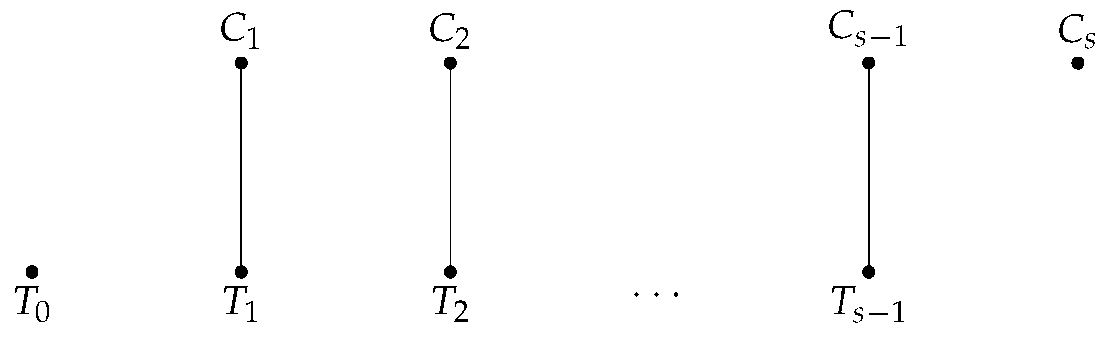
The backward correction in Algorithm 2 is further illustrated herein. Suppose that we have already matched the first s treated units, and no free control is available to match the next treated unit $T_0$. Pick any feasible control in this list, such as $C_1$. This control has already been matched with a treated unit, such as $T_1$ (see Figure 1). The joint list of feasible controls for $T_0$ and $T_1$ may or may not contain a free control. If it does, then this free control is matched with $T_1$. This frees $C_1$, which can be matched with $T_0$, increasing the number of matched units by one. If not, then pick any feasible control in the list of $T_1$, such as $C_2$, and look for a free control in the joint list of $T_0$, $T_1$, and $T_2$. This procedure can be repeated for a maximum of s steps. If a free control is found during the process, then the number of matches increases from s to $s+1$. If not, then the treated unit is left unmatched.

Algorithm 2: Algorithm for backward correction.

The algorithm does not specify how to pick the controls when more than one is available. Different selection rules can lead to different order-optimal matchings, but all matchings share the same subset of treated units, which is the order-optimal element of Gale’s theorem. If the controls are sampled uniformly at random, then the algorithm complexity is $O\left(n^2\right)$, as shown in Appendix A. For our matching strategy, the selection rule leads to an order-optimal matching of a minimum cost (see the next section).

An Example with a Few Units

We close this section with a simple example illustrating both Algorithm 1 and its implementation in the R environment [13]. Consider the cost matrix in Figure 2. The matching problem requires five treated units to be matched with four control units, and thus a complete matching is not possible. The order-optimal element is $\{t_1,t_2,t_3,t_5\}$, and it is found after using the backward correction algorithm twice. Two order-optimal matchings can be built on the order-optimal element, as shown in Figure 3.

Classic cost-optimal matching can be implemented in R with the optmatch package [5]. For order-optimal matching, we built the package OSDR [14]. The main function of OSDR is running Algorithm 1. To find the order-optimal matching in R, we gave as input the ordered list of controls. The function output contains (1) OSDR (a random order-optimal matching), (2) matched (the index of matched units), and (3) unmatched (the index of unmatched units). The example above can be run in R as follows:

# M is a list of within-caliper control units

M1<-c(‘‘c1’’,‘‘c2’’,‘‘c3’’)

M2<-c(‘‘c1’’,‘‘c3’’)

M3<-c(‘‘c2’’)

M4<-c(‘‘c1’’,‘‘c3’’)

M5<-c(‘‘c1’’,‘‘c4’’)

M  <-list(M1,M2,M3,M4,M5)

OSDR(M)

$OSDR

[1] ‘‘c1’’ ‘‘c3’’ ‘‘c2’’ ‘‘0’’  ‘‘c4’’

$matched

[1] 1 2 3 5

$unmatched

[1] 4

Finally, we can save the restricted list of matchable treated units, M[[OSDR$matched], and find the cost-optimal matching for this list, such as with the calling function pairmatch from package optmatch. This matching strategy finds a minimum cost matching on the order-optimal element, and it is discussed in the next section.

2.4. An Optimal Matching Strategy

In this section, we propose a matching strategy which compromises between order- and cost-optimal optimality. Before proceeding, we analyze the relation between these two types of optimal matchings. In the example from the previous section, the cost- and order-optimal matchings were the same size. This is true in general, as we prove in the next proposition.

Theorem 3.

Order- and cost-optimal matchings are maximum size matchings.

Proof. 

Let $M_C$ and $M_O$ be cost- and order-optimal matchings, respectively. Since $M_C$ is a maximum size matching, we have $\mid M_O\mid \le \mid M_C\mid$. Suppose that $M_O$ matches fewer treated units than $M_C$. Then, since $M_C$ is built on a matchable subset of treated units, it follows from the definition of a matroid that one more treated unit can be added to $M_O$ to obtain a larger matching. The previous property can be used until $\mid M_O\mid =\mid M_C\mid$.    □

Thus, in the set of maximum size matchings, the subsets of order- and cost-optimal matchings do not necessarily intersect. If they do, then any matching in the intersection is both a cost- and order-optimal matching. Thus, these matchings are, in a sense, “doubly” optimal. Instead, any matching outside the intersection sacrifices either the cost or order optimality. The following matching strategy leads to a doubly optimal matching when it exists. Otherwise, it returns an order-optimal matching of a minimum cost.

The strategy consists of two steps:

• Find the matchable subset which is order optimal under Definition 2;
• Find the minimum-cost matching for this subset.

In comparative studies, the matched subsets are finally used to compare the outcome variables across the two groups. A common measure of the difference between the outcomes is the average treatment effect on the treated units (ATT). Suppose that we have a sample of $n_T+n_C$ units, and let n be the common size (according to Proposition 3) of the cost- and order-optimal matching. Also, let

$$(a_1,\cdots ,a_n)\mathrm{and}(a_1^{\prime },\cdots ,a_n^{\prime })$$

be the matched treated and control index sets from the cost-optimal matching, respectively, and

$$(b_1,\cdots ,b_n)\mathrm{and}(b_1^{\prime },\cdots ,b_n^{\prime })$$

be the corresponding sets obtained from the order-optimal matching. Then, we have

$${\widehat{ATT}}_{cost}=\frac{1}{n}\sum _1^n(y_{a_i}-y_{a_i^{\prime }})\mathrm{and}{\widehat{ATT}}_{ord}=\frac{1}{n}\sum _1^n(y_{b_i}-y_{b_i^{\prime }}).$$

(1)

In the case of a complete matching, all $n_T$ treated units in the sample are matched in both the order- and cost-optimal matching. However, the matched controls $c_{a_i}$ and $c_{b_i}$ may be different. When a complete matching is not possible ($n<n_T$), both the treated and control units in the two matchings may differ. The matching strategy described above finds the controls of a minimum cost for the order-optimal subset. Thus, if the matching is complete, then the $ATT$ estimate found with this strategy is clearly the same as that for the cost-optimal matching; otherwise, the $ATT$ estimate is generally different.

2.5. Simulation Study

We performed a small simulation to investigate the performance of the proposed matching strategy in the case of incomplete matching. The population ($N=1000$) was generated as follows. We simulated a single covariate $X\sim U(0,1)$. The covariate was a confounder: it was associated with both the binary treatment T and the outcome variable Y. As for T, we assumed that $P(T=1)$, the probability of being treated, increased with X. The outcome Y was assumed to be normally distributed, with the mean depending on the treatment status. We assumed that $Y\left(0\right)$, the potential outcome under no treatment, was roughly constant, while $Y\left(1\right)$, the potential outcome under treatment, was an increasing function of X.

A random sample was available from the population. From the sample units, we knew the values of X, T, and the observed outcome $Y=Y\left(0\right)(1-T)+Y\left(1\right)T$. Notice that since $P(T=1)$ is increasing in X, we generally observed samples with higher numbers of treated units, and thus a complete matching was not possible. For each sample, we calculated the matching imbalance (measured by the average pair distance for the matching), the $ATT$ estimates using Equation (1), and their simulation standard error. The latter was implemented, giving higher matching priority to units with higher X values. The results are shown in

Table 1. Performance measure for cost- and order-optimal matching ($n=10$).

Statistic 1	Cost Optimal	Order Optimal
Imbalance	1.18	1.34
$\widehat{ATT}$	1.94	2.17
sd($\widehat{ATT}$)	0.62	0.70

¹ Average over 100 replications. (true) $ATT\approx 2.1$.

,

Table 2. Performance measure for cost and order optimal matching ($n=20$).

Statistic 1	Cost Optimal	Order Optimal
Imbalance	2.70	3.37
$\widehat{ATT}$	1.98	2.19
sd($\widehat{ATT}$)	0.49	0.51

¹ Average over 100 replications. (true) $ATT\approx 2.1$.

and

Table 3. Performance measure for cost and order optimal matching ($n=30$).

Statistic 1	Cost Optimal	Order Optimal
Imbalance	4.00	5.60
$\widehat{ATT}$	1.95	2.29
sd($\widehat{ATT}$)	0.40	0.42

¹ Average over 100 replications. (true) $ATT\approx 2.1$.

. Cost-optimal matching was less imbalanced (by design for each sample and thus also on average) and had less variability across the samples on average compared with order-optimal matching, which showed a lower bias.

The average lower bias from order-optimal matching was due to the choice of the “right” matching priority, as choosing a random priority would give the same average bias for both cost- and order-optimal matching. In other words, the technique can be advantageous when we have additional information about the correlation structure of the covariate, treatment assignment, and outcome that can be turned into a sensible matching priority.

In the next section, we present a case study about the salary gap across male and female executives where the matching priority is suggested by the literature on the salary gap. The resulting order-optimal matching for the gender gap study (shown in Figure 4) had an average matching cost of 2.21, which was higher than the average matching cost of the cost-optimal matching (1.77). The difference can be considered the price paid for matching units with higher priority.

3. Case Study

In this section, we expose a case study arising from a consultancy given to a firm offering services for health resource management. The research project focused on the gender gap and required a comparison of several work outcomes across male and female workers. Since the classic work of [15], statistical analysis based on matched pairs has increasingly been used in diversity management studies. Matching women and men having the same job characteristics has a strong intuitive appeal, and it also guarantees separation of the design stage (where matched pairs are obtained) from the analysis stage (where the outcomes are compared).

3.1. Data Description

The research project required a comparison of several work outcomes across male and female workers. The project involved several firms in different sectors, and a sample was extracted from each of them. Sample sizes were based on the sustained cost of research and varied from 100 observations (for the firms commissioning the research) to 20 observations for smaller firms. The average non-response rate was about 30%, and the company sample sizes ranged from 16 to 80 observations. The procedure for collecting sample information involved the use of archival data via randomized stratified sampling. The sampling strata were given by the following variables: age (years), position (top manager = 4, middle manager or executive = 3, and first-line manager or supervisor = 2), education (post-graduate = 5, graduate = 4, and high school = 3), contract type (fixed term = 4 and permanent = 3), and seniority (years in the position). For the outcome analysis, a questionnaire was distributed to retrieve information about wages and detailed compensation components. Moreover, interviews were also carried out, targeting information on the organizational climate and working attitudes which could not be obtained otherwise. The sampling mechanism reflected the true sex proportion in the population, resulting in several samples having more women than men (see

Table 4. Sample size for gender gap study.

Firm ID	Sector	Number of Men	Number of Women	Sample Size
1		16	10	26
2		6	10	16
3		7	16	23
4		9	3	12
5		12	15	27
6		13	13	26
7		7	4	11
8		10	12	22
9		1	0	1
10		1	0	1
11		34	27	61
12		1	3	4
13		1	6	7
14		9	11	20
15		11	16	27
16		18	44	62

).

3.2. Methodology

There is evidence from the gender studies literature that the gender gap increases with one’s position in the organizational hierarchy, with the greatest differences being at the highest executive levels, where the pay levels and the variable part of remuneration vary more (see [16] for a review), and thus it is desirable to include women in the analysis. However, for most of the firms analyzed, classic cost-optimal matching resulted in dropping some of the women in apical positions due to either caliper restriction, the structural prevalence of women over men, or both. Instead, we used an order-optimal matching algorithm to give matching priority according to the executive rank.

3.3. Data Analysis

We describe the analysis for firm number 15, a company with a strong prevalence of female executives (see Table 4). A complete matching was not possible, but it was desired to lose as few women in apical positions as possible. The female executives were first ordered by (decreasing) position in the organizational hierarchy. In case of ties, seniority was used to break the tie. Then, we applied the two-step strategy illustrated in Section 2.4. We restricted the data set to the order-optimal subset, and we sought out the cost-optimal matching for that subset.

The matched subsets from order- and cost-optimal matching are compared in

Table 5. Order- and cost-optimal matched subsets for the gender gap study. Women IDs are ordered by matching priority (1 = highest).

ID	1	2	3	4	5	6	7	8	9	10	11	12	13	14	15	16
Cost Optimal	0	1	1	1	0	1	1	1	1	1	1	1	0	0	1	0
Order Optimal	1	1	1	1	1	1	1	1	1	1	1	0	0	0	0	0

. Both had the same (maximum) size, but they differed in two units. Specifically, the order-optimal matching comprised female executives from $t_1$ to $t_{11}$, while the cost-optimal matchings excluded $t_1$ and $t_5$ and included $t_{12}$ and $t_{15}$. Executives $t_1$ and $t_5$ were higher in the hierarchy, which is desirable under the study’s hypothesis. However, their inclusion caused an increase in the covariate distance between the two groups. To evaluate this cost, we calculated the sum of the matched distances for the two matchings. The average matching distance increased from $1.73$ to $2.21$ ($3.68$ in standard deviation units), and thus this was the imbalance resulting from including executives $t_1$ and $t_5$ in the matched subset.

The matchings are represented in Figure 4. The final matching was the input for the outcome analysis, where several comparisons between the male and female executives were carried out. Even if the imbalance difference were relatively small, it was not clear whether the inclusion of higher-ranked women was worth the greater imbalance. As noticed earlier, the literature suggests that the inclusion of highly ranked female executives is important, and the matching priority was carried out accordingly. Obviously, we do not know the true correlation structure between the executive rank, sex, and work characteristics, which suggests that the final estimates should be taken cautiously. We return to this issue in the Discussion section.

4. Discussion

In this work, we proposed an optimal matching strategy for matching units according to a given priority. The strategy is based on a combinatorial result from D. Gale, proving the existence of an order-optimal matching and algorithmic proof thereof. The matching is optimal in the sense that no other matching of the same size can contain a unit with a higher matching priority. The matching priority essentially gives zero weight to some pair matchings, favoring matched pairs with higher-priority units. We illustrated order-optimal matching in a case study comparing female and male executives. In this case, it was presumed that the inclusion of specific pairs in the final matching was important, and thus we used this information to set the matching priority.

We observed that the idea of giving different weights to sample units in estimation problems is quite ubiquitous, and alternative techniques exist to avoid drop-offs. Whenever possible, the problem can be avoided with a careful design phase. Unequal probability sampling [17] can be used when it is known in advance that a subset of the population is not going to be adequately represented in the sample. This is common practice when a population subset is believed to be more important for the estimation. After the data collection phase, post-correction can be performed using importance sampling [18]. In comparative studies involving matching, the most common approach for avoiding drop-offs is probably matching with replacement [19], and it has many variations, including the recent development of the synthetic control method [20]. This technique stems from a different philosophy as it allows resampling units. Analytical results are available for its asymptotic behavior. In large samples, the estimates obtained with replacement showed a bias and variance trade-off compared with matching without replacement [19].

In causal inference, the term optimal matching usually refers to minimum-cost matching. P. Rosenbaum [3] pioneered minimum cost flow algorithms as the key tool for finding an optimal matching between treated variables and their controls. We showed that order- and cost-optimal matching had the same (maximum) size, but they did not necessarily coincide. Despite the covariate balance of an order-optimal matching not being able to be lower than the covariate balance achieved by a cost-optimal matching, it is possible to obtain better estimates from order-optimal matching in particular situations. This happens when we have a sensible matching priority. A simulation study showed that less biased estimates were obtained when the treatment effect increased with the matching covariate.

A limitation of order-optimal matching is that it is not always possible to know the correlation structure for deciding the matching priority. This information is generally unavailable in empirical studies. In similar cases, estimates must be performed carefully as they depend on a belief about the covariance structure. The simulation provided is illustrative of a special case, but it is limited in scope. A full assessment of the pros and cons of order-optimal matching versus cost-optimal matching would require a larger simulation effort exploring several scenarios for the covariance structure of the outcome and the covariates.