Abstract
Accurate vehicle detection is crucial for the advancement of intelligent transportation systems, including autonomous driving and traffic monitoring. This paper presents a comparative analysis of two advanced deep learning models—YOLOv8 and YOLOv10—focusing on their efficacy in vehicle detection across multiple classes such as bicycles, buses, cars, motorcycles, and trucks. Using a range of performance metrics, including precision, recall, F1 score, and detailed confusion matrices, we evaluate the performance characteristics of each model.The findings reveal that YOLOv10 generally outperformed YOLOv8, particularly in detecting smaller and more complex vehicles like bicycles and trucks, which can be attributed to its architectural enhancements. Conversely, YOLOv8 showed a slight advantage in car detection, underscoring subtle differences in feature processing between the models. The performance for detecting buses and motorcycles was comparable, indicating robust features in both YOLO versions. This research contributes to the field by delineating the strengths and limitations of these models and providing insights into their practical applications in real-world scenarios. It enhances understanding of how different YOLO architectures can be optimized for specific vehicle detection tasks, thus supporting the development of more efficient and precise detection systems.
1. Introduction
A rapid increase in vehicles on the road has created challenges in traffic management, requiring accurate vehicle detection and counting for effective traffic control. Vehicle detection, which is vital for real-time estimation of types and total counts of vehicles, involves localization to provide the locations of vehicles and classification to identify their categories [1]. Vehicle detection is a crucial application in computer vision, with wide-ranging uses in traffic monitoring, autonomous driving, security, and environmental management. Various challenges can significantly influence the accuracy of vehicle detection. Variations in lighting conditions can alter the appearance of vehicles in images or videos, making detection inconsistent. The presence of obstacles, such as other vehicles, buildings, or trees, can obscure vehicles wholly or partially. Furthermore, diversity in vehicle colors, shapes, and sizes adds complexity to detection processes. Viewing angles also affect the consistency of vehicle appearances, with different perspectives like the front, rear, and side posing unique challenges. Image or video quality, particularly low-resolution or blurry media, can impair the precision of detection models. Lastly, extreme weather conditions such as heavy rain, fog, or snow can drastically reduce visibility, further complicating the detection of vehicles.
Traditionally, methods like the histogram of oriented gradients (HOG) have been used to implement vehicle detection [2]. These traditional approaches often involve complex workflows, significant manual intervention, and lengthy processing times. To overcome these challenges, convolutional neural networks (CNNs) have been introduced, demonstrating superior performance [3,4,5]. Further advancements in this field have led to the development of region-based convolutional networks (R-CNN), Fast R-CNN, Faster R-CNN, and region-based fully convolutional networks (R-FCN), which employ a two-stage detection process. This process begins with the generation of region proposals and is followed by their refinement through localization and classification [6,7,8,9,10].
Given the computational complexities, slower inference speeds, and resource limitations of the previously mentioned models, the one-stage detection approach has gained popularity. This method identifies objects in a single iteration by predicting bounding box locations and assigning labels to detected objects [11]. The Single Shot Multibox Detector (SSD) leverages convolutional features across multiple scales to predict bounding boxes and class probabilities. RefineDet++ [12] enhances accuracy by merging improved feature extraction with precise boundary determination. The Deconvolutional Single Shot Detector (DSSD) [13] uses deconvolutional layers to restore spatial data lost during feature pooling, while ResNet manages class imbalances effectively with focal loss.
You Only Look Once (YOLO ) stands out for its simple architecture, high accuracy, and rapid inference speed among single-stage detectors. YOLOv1 employs a 24 layer convolutional network with 2 fully connected layers, and a streamlined variant, Fast YOLO, features 9 convolutional layers, with both built on Darknet. YOLOv2 improves upon this with batch normalization, anchor boxes, a depth-classifying feature, dimension clusters for anchor sizing, and fine-grained features to detect smaller objects, using Darknet-19 instead of the more complex VGG-16 or less accurate GoogleNet [14,15]. YOLOv3 further deepens the architecture and refines feature extraction using Darknet-53 coupled with residual networks, and it shifts from SoftMax to binary cross-entropy for more versatile box labeling [16].
YOLOv4 and YOLOv5 continue this evolution by enhancing both speed and accuracy. YOLOv4 integrates advancements in the backbone network (CSPDarknet53), a neck module for feature integration (PANet with SPP), and a predictive head based on the YOLOv3 architecture [17]. YOLOv5, built on PyTorch, simplifies the model for better user accessibility and further speeds up performance using a new CSP-Darknet53 backbone, SPPF, and a new CSP-PAN neck. YOLOv6 and YOLOv7 focus on reducing computational demands and improving precision, respectively, with YOLOv7 introducing auxiliary and lead heads for enhanced training and output accuracy [18,19].
YOLOv8 expands the framework to support a variety of AI tasks such as detection, segmentation, and tracking, enhancing its versatility across multiple domains. It features a modified CSPDarknet53 backbone and a PAN-FPN neck. YOLOv9 and YOLOv10 introduce cutting-edge techniques like programmable gradient information (PGI) and the generalized efficient layer aggregation network (GELAN), with YOLOv10 eliminating the need for non-maximum suppression (NMS) through an end-to-end head, facilitating real-time object detection [20,21].
This study aims to compare the performance of YOLOv8 and YOLOv10 for vehicle detection, focusing on their effectiveness in various challenging environments. Given the advancements in one-stage detection algorithms, it is crucial to evaluate how these newer models perform in terms of accuracy, speed, and computational efficiency. This analysis will help identify which model delivers superior performance and under what conditions, providing valuable insights for applications in autonomous driving, traffic management, and other related fields.
The remainder of this work is organized as follows. The literature related to this study is thoroughly discussed in the Section 2, which provides a comprehensive overview of the developments in vehicle detection technologies, especially focusing on the evolution of YOLO architectures. The Section 3 details the workflow and mechanisms behind YOLOv8 and YOLOv10, elaborating on their technical specifications and implementation strategies. Finally, in the Section 4 and Section 5, exploratory data analysis is conducted, and performance matrices are evaluated and discussed, highlighting the comparative strengths and weaknesses of the models.
2. Literature Review
In the field of computer vision, the ability to accurately detect and track vehicles has become increasingly vital across various applications, from traffic management to autonomous driving. Over the years, technology has evolved from basic detection algorithms to sophisticated neural networks capable of performing complex vehicle recognition tasks under a variety of conditions. This literature review explores the progression from early vehicle detection methods to the latest advancements in YOLO, highlighting significant contributions and innovations which have shaped current practices in vehicle monitoring systems.
Vehicle detection and tracking are critical components of computer vision-based monitoring systems, facilitating tasks such as vehicle counting, accident identification, traffic pattern analysis, and traffic surveillance. Vehicle detection involves identifying and locating vehicles using bounding boxes, while tracking entails following and predicting vehicle movements through trajectories [22]. Initially, convolutional algorithms focused on background removal and feature extraction defined by users, but these faced difficulties with dynamic backgrounds and variable weather conditions [23]. To address these issues, Barth et al. introduced the Stixels method in their research, which utilizes color schema to convert movement information [24]. Convolutional neural networks (CNNs) have been adopted to overcome obstacles such as obstructive objects, varying backgrounds, and processing delays, enhancing accuracy in the process [6]. Various papers have explored CNN architectures tailored to these tasks, including the RCNN, FRCNN, SSD, and ResNet [7,25,26,27,28,29,30,31,32,33]. Additionally, Azimjonov and Özmen compared traditional machine learning and deep learning algorithms for road vehicle detection [11]. For vehicle tracking, these methods include tracking by detection using bounding boxes and appearance-based tracking focused on visual features. Among these, the combination of YOLO for detection and a CNN for tracking has shown superior performance compared with nine other machine learning models, demonstrating a robust approach for vehicle monitoring systems.
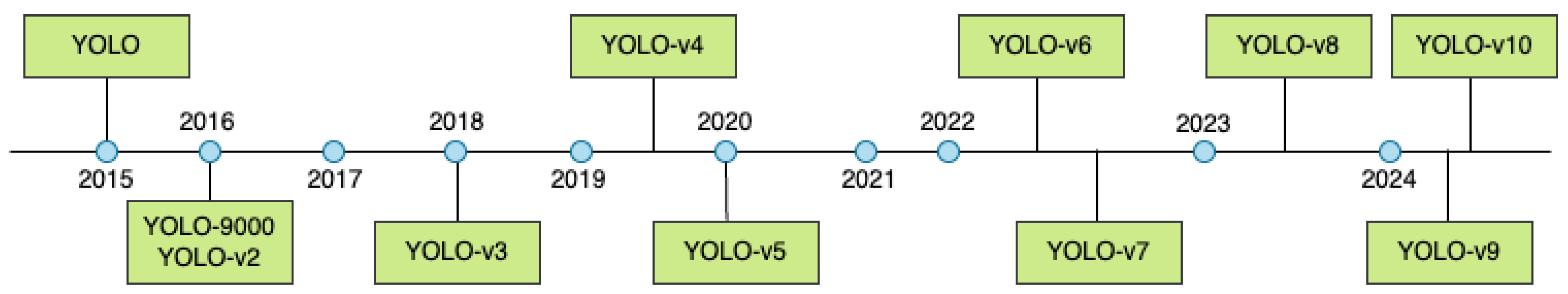
YOLO, by approaching vehicle detection as a regression task using convolutional neural networks (CNNs), has significantly improved the accuracy of detecting the locations, types, and confidence scores of vehicles. It also enhances detection speed while managing blur during movement by providing bounding boxes and class probabilities. Figure 1 shows a comprehensive visual overview of the progressive enhancements in the YOLO architecture series from YOLOv1 to YOLOv10. YOLOv2, leveraging GPU features and the anchor box technique, improved upon its predecessor in the detection, classification, and tracking of vehicles [34]. Ćorović, Ilić et al. proposed YOLOv3, which was trained for five classes, including cars, trucks, street signs, people, and traffic lights. It was proposed to detect traffic participants effectively across various weather conditions [35]. YOLOv4 focused on enhancing the detection speeds of slow-moving vehicles in video feeds [36], while YOLOv5 utilized an infrared camera to locate heavy vehicles in snowy conditions, facilitating real-time parking space prediction due to its efficient framework and fast identification capabilities [37]. Furthermore, YOLOv6 introduced an enhanced network architecture and training methods to achieve superior accuracy in real-time detection [38]. Modifications in YOLOv7 were tailored for detecting, tracing, and measuring vehicles on highways, improving decision making and tracking in urban settings [39,40]. Future iterations of YOLO are expected to incorporate features such as lane tracking and velocity estimation to further enhance the accuracy and utility of the system in diverse driving environments.

Figure 1.
Evolution of the YOLO architecture.
In their research, Soylu and Soylu explored the development of a traffic sign detection system using YOLOv8, which was enhanced with a spatial attention module (SAM) for better feature representation and a spatial pyramid pooling (SPP) module to capture vehicle features at multiple scales, aiming to improve road safety and efficiency in autonomous vehicles [41]. YOLOv8m, with 295 layers and while processing images of 1280 pixels, achieved impressive accuracies of 99% in mAP-50 and 83% in mAP-50-95. Further optimizations could involve simplification, fine-tuning, and pruning of the model. Future enhancements may integrate natural language processing to extend YOLOv8’s capabilities. Additionally, this model has improved vehicle detection in segmented images by employing advanced feature extraction techniques such as the scale-invariant feature transform, oriented FAST and rotated BRIEF, and KAZE, followed by training with a deep belief network classifier, achieving accuracies of 95.6% and 94.6% on the Vehicle Detection in Aerial Imagery and Vehicle Aerial Imagery from a Drone datasets, respectively. Increasing vehicle categories and integrating additional features could further enhance classification accuracy [42].
In comparison, YOLOv10, although faster in post-processing due to its non-maximum suppression (NMS) free approach, which reduces latency, tends to miss smaller objects because of fewer parameters and lower confidence scores [43]. Each iteration of YOLO has seen enhancements in inference speed and overall performance. While earlier versions like YOLO and YOLOv3 struggled with vehicle visibility in severe weather, YOLOv5 proved effective under cold conditions. YOLOv8 and YOLOv10 have the potential to further refine feature extraction techniques to better cope with adverse weather. These models have traditionally struggled with detecting small and occluded objects due to their fixed grid structure. However, YOLOv8 improved the detection of smaller objects through advanced feature extraction, and YOLOv10 adopted multi-resolution techniques and an anchor-free approach. While older YOLO models grappled with inaccuracies in complex scenarios due to higher frame rates, YOLOv8 implemented model quantization to balance accuracy with real-time performance, and YOLOv10 employed a complex architecture with lightweight layers to maintain precise detection capabilities.
In conclusion, the literature review underscores the rapid advancements in vehicle detection technologies, particularly within the YOLO series, from basic detection to sophisticated systems capable of handling complex scenarios and adverse conditions. The progression from YOLO to YOLOv10 highlights a continual improvement in speed, accuracy, and adaptability, addressing previous limitations such as poor visibility in bad weather and difficulty detecting small or occluded objects. These developments set a solid foundation for this study, which aims to delve deeper into the capabilities and performance of YOLOv8 and YOLOv10, focusing on their application in real-world vehicle detection scenarios. By comparing these models, this research seeks to identify optimal solutions which may significantly enhance the efficacy of automated systems in traffic management and autonomous driving.
3. Methodology
3.1. Dataset
The dataset for this study was sourced from the open source repository ‘GitHub—MaryamBoneh/Vehicle-Detection: Vehicle Detection Using Deep Learning and YOLO Algorithm’ [44]. This dataset has a total of 1321 images, where the train folder has 1196, the test folder has 8, and the validation folder has 117. Each image has a resolution of 416 × 416 pixels. The images are already annotated with 5 classes as follows: car, motorcycle, truck, bus, and bicycle. Sample images of the collected dataset are shown in Figure 2.
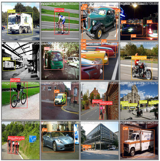
Figure 2.
Sample images from the dataset [44].
3.2. Data Augmentation
Data augmentation is an important process in deep learning models in computer vision. Augmentation adds more images to the existing images to increase the size of the dataset. By performing augmentation, a machine can learn a wider variety of scenarios in order to capture the essence of unseen versions of data, thereby reducing overfitting. In order to avoid underrepresented classes, data augmentation can be used to generate more samples, thereby tackling issues in imbalanced classes and ensuring unbiased representation. Adding noise helps a machine learn variations in real-world applications and learn from different examples, increasing the accuracy of models. Collecting a large amount of data in real time is impractical, and this can be overcome by using augmentation to provide many images.
When detecting or classifying a vehicle, light conditions, weather changes, partial or full occlusion, and different angles are challenges. Data augmentation addresses these issues by diversifying the training dataset. It introduces variations such as different light variations and angles and can even add occlusions to images. By using augmented data, models learn to identify objects better, enhancing their ability to detect and classify vehicles accurately in different settings. This approach not only improves the performance of models but also increases robustness.
3.2.1. Random Crop
Cropping increases the flexibility of a model by ensuring that the model can detect vehicles even if the vehicles are not visible fully (when part of the image is missing or when vehicles appear larger), scaled uniformly, or at different distances from the camera. Here, the images were cropped with 0% minimum zoom, where the original image was retained as given, and with 20% maximum zoom, meaning about 20% of the dimensions of the images were cropped from each side. The cropped image might range from 332 × 332 pixels for 20% maximum zoom to 416 × 416 pixels for 0% minimum zoom, making cropping more effective in real-world cases where vehicles may not always appear with the same position, size, or shape. To crop 20% of each side of the images, Equation (1) was used:
3.2.2. Random Rotation
The image rotated between −15 and +15 degrees in direction, shifting the positions of the vehicles in the image (Equation (2)). The bounding box had to be adjusted to include a vehicle perceived from a different angle. When using rotating cameras, the vehicles might not be aligned in the frames, where the vehicles might appear in a rotated view. Hence, various angles could be taken into consideration for better learning:
Equation (3) illustrates the rotational transformation of a two-dimensional image:
where denotes the rotation matrix.
3.2.3. Random Shear
Shearing the image by ±10 degrees horizontally (x axis) and vertically (y axis) resulted in geometric distortion, providing different perspectives:
where S is the shear matrix.
3.2.4. Random Grayscale
This technique converts 15% of colored images to grayscale, where the models learn to prioritize shape and texture over color. Equation (5) displays the process of transformation from color to grayscale:
3.2.5. Saturation
Adjusting saturation introduces a varied color intensity (based on light variations), improving the ability of models to use different colors. The formula for saturation contains a saturation adjustment factor (), ranging here between −25% and +25% (Equation (6)):
3.2.6. Brightness
Brightness augmentation is beneficial as a model needs to handle different brightness levels to denote various weather conditions. In this study, the brightness of the dataset was adjusted between −15% and +15% (Equation (7)):
Here, denotes the brightness adjustment factor, ranging between −0.15 and +0.15.
3.2.7. Blur
Blur is used to reduce the sharpness and contrast of images. Here, blur applies a blurring effect in which the blur kernel size can vary by up to 2.5 pixels. This process can help in vehicle detection by reducing noise and increasing feature extraction, thereby increasing the accuracy of vehicles in an image:
wherein illustrates the standard deviation of the Gaussian blur kernel.
3.2.8. Random Noise
Introducing noise to images intentionally alters the pixel values, causing black and white spots in unexpected areas of images while implementing noise affecting 0.1% of the pixels in an image. N is the noise added to the original image in Equation (9):
3.2.9. Hue, Saturation, and Value (HSV)
Hue, saturation, and value (HSV) is used to control the brightness of an image. It is a parameter for adjusting the levels of hue, saturation, and value (HSV) for a color, where hue represents a color type, saturation denotes the intensity of a color, and value indicates the brightness of a color. Here, hsv_v = 0.4 was used to scale the brightness down to 40% in order to create variations in brightness:
where is the adjusted brightness of a pixel.
3.2.10. Translate
Translate signifies the translation transformation of an image, involving shifting an image along the horizontal and vertical axes. In this work, a translate value of 0.1 shows that the images can be shifted horizontally and vertically by 10% of their width and height, respectively:
where and are the translation factors.
3.2.11. Mosaic
The mosaic augmentation technique combines four images by dividing them into quadrants and combining their parts. A value of 1.0 means that the mosaic approach is applied to the dataset:
where is the intensity of one of the four images; and are coordinates in the mosaic image; and and are the corresponding coordinates in the source image.
3.2.12. Random Erasing
The erasing method erases or occludes parts of an image. An erasing value of 0.4 indicates that 40% of the image is erased:
where I(x, y) is the intensity of the original image and indicates the intensity of the pixel after random erasing.
These augmentation processes are important in vehicle detection because they increase the dataset size and help a machine understand that real-life scenarios are different.
3.3. YOLOv8 Architecture
YOLOv8 builds upon the foundation set by YOLOv5, introducing significant enhancements in its architecture to boost detection precision. Central to its design is the transition to an anchorless architecture through incorporation of the C2f module. This module seamlessly integrates complex features with contextual information, thereby increasing the accuracy of the model. By eliminating traditional anchor boxes, which often fail to represent the diverse pattern distributions in datasets accurately, YOLOv8 simplifies the prediction of bounding boxes and streamlines post-processing activities, notably reducing the dependency on non-maximum suppression [21,45]. Table 1 outlines the architecture of YOLOv8, illustrating the configuration of each layer, the type and size of filters used, and the output dimensions at each stage. Notably, the architecture integrates the innovative C2f module and spatial pyramid pooling fractional (SPPF) approach to enhance feature representation and localization accuracy.

Table 1.
YOLOv8 architecture.
In the output layer, YOLOv8 utilizes a combination of sigmoid and softmax activation functions. The sigmoid activation function determines the probability of a bounding box containing an object, while the softmax function classifies the object into one of the predefined categories.
Further refinements include implementation of the complete intersection over union (CIoU) and distribution focal loss functions, which are specifically designed to enhance a model’s accuracy in locating and sizing bounding boxes. These functions are particularly effective in handling smaller objects, a notable challenge in previous YOLO versions. Additionally, binary cross-entropy is used for calculating classification loss, ensuring a robust approach to multi-class categorization.
The performance metrics indicate that YOLOv8x, an advanced variant of the model, demonstrated superior capability on the MS COCO dataset test-dev 2017. It achieved an impressive average precision of 53.9% for images resized to 640 pixels, while processing at a remarkable speed of 280 frames per second when accelerated by TensorRT on an NVIDIA A100 GPU.
3.4. YOLOv10 Architecture
YOLOv10 advances the field by setting a new benchmark in inference speed, notably by eliminating non-maximum suppression (NMS) from its post-processing stages. It employs a novel NMS-free approach which integrates dual-label assignment, balancing thorough supervision via the one-to-many branch and rapid inference through the one-to-one branch. This model also introduces a standardized matching method to ensure consistency between these dual branches, optimizing both the training and inference processes [21,46]. Table 2 outlines the architecture of YOLOv10, detailing the configuration of each layer, the type and size of filters employed, and the output dimensions achieved at each stage. This architecture is characterized by its innovative use of the partial self-attention (PSA) and spatially constrained (SC) layers, which enhance the model’s efficiency and precision. The model notably includes advanced feature integration techniques such as depthwise and pointwise convolutions, combined with a sophisticated mechanism for dual-label assignment to optimize both the training and inference phases. These design choices underscore YOLOv10’s advanced capabilities in handling complex object detection tasks with improved accuracy and speed.
Table 2.
YOLOv10 architecture.
The model’s architecture is designed to increase efficiency without sacrificing performance. This is achieved by focusing on a lightweight classification head to address the regression task bottleneck. Additionally, the integration of pointwise convolution elevates the channel dimensions, while depthwise convolution, which lowers the resolution, has been shown to improve the average precision by 0.7%. Furthermore, the inclusion of a depthwise layer within a compact inverted block has been shown to boost the average precision by an additional 0.3%. The model combines these features with a rank-guided block design for a compact structural approach.
The precision-centric aspects of YOLOv10 suggest that large-kernel convolutions are particularly beneficial for smaller models as they expand the size and receptive field. Moreover, partial self-attention mechanisms are implemented to link effective global modeling with minimal computational overhead, thus reducing the complexity typically associated with full self-attention.
4. Experimental Results
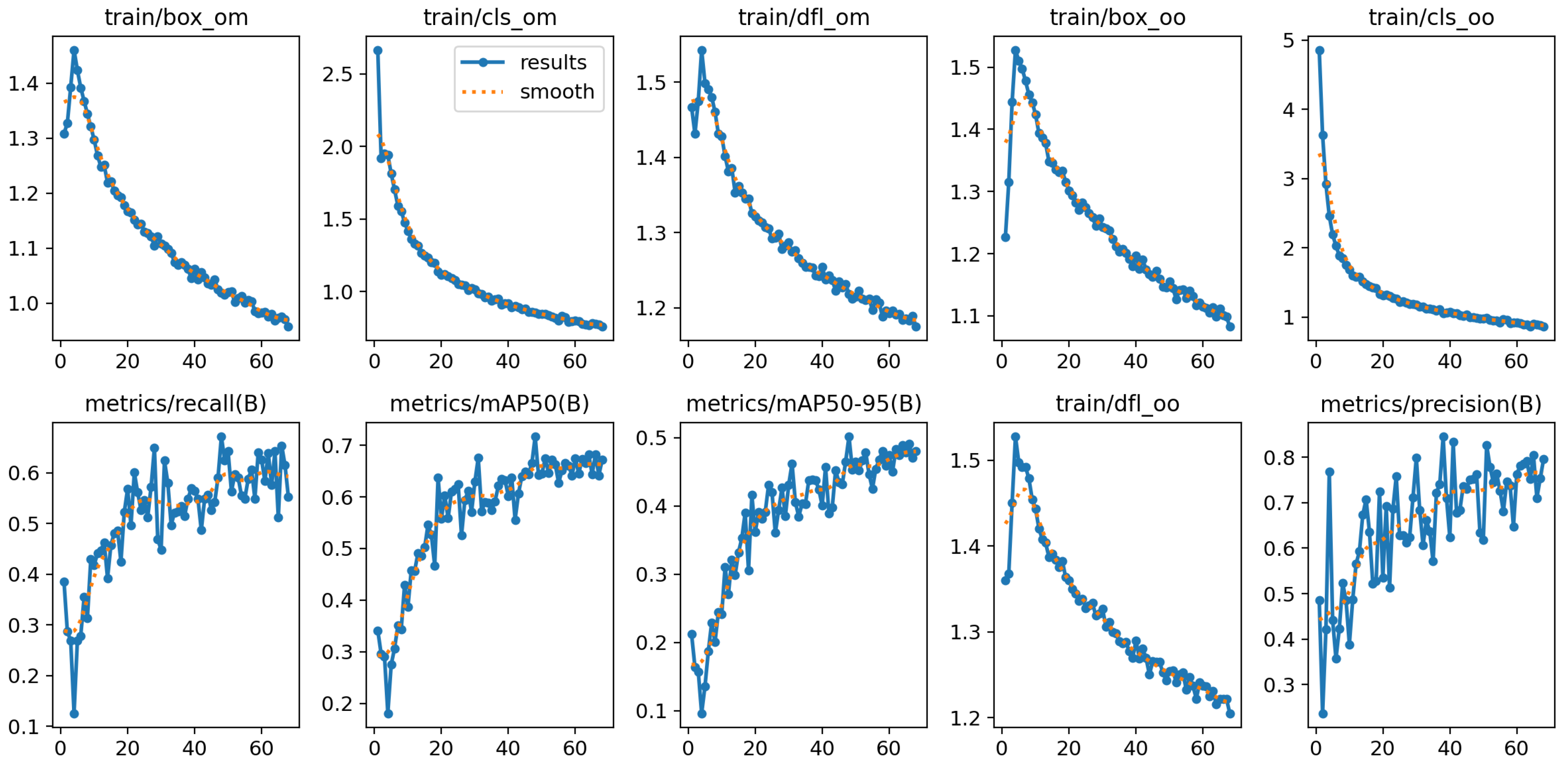
The experimental results for the YOLOv8 and YOLOv10 models, detailed in Figure 3 and Figure 4, highlight their performance across various metrics throughout the training and validation phases. Both models were trained and validated in a PyTorch environment on a high-performance system equipped with NVIDIA GPUs when using cutting-edge deep learning techniques. The hyperparameters were meticulously fine-tuned over 1000 epochs to enhance model accuracy and efficiency. The stochastic gradient descent (SGD) optimizer was employed with an initial learning rate of 0.01 and a momentum value of 0.9. A decaying learning rate strategy complemented by specific regularization settings optimized performance. Notably, the group parameters were adjusted to ensure some weights experienced no decay (decay = 0.0), while the biases were subjected to L2 regularization (decay = 0.0005). This regimen helped minimize overfitting and maintain generalizability. The batch size was set to 16 to balance computational efficiency with accuracy.
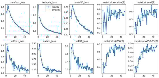
Figure 3.
Performance of YOLOv8 model.
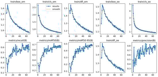
Figure 4.
YOLOv 10 model’s performance.
The training was executed for up to 1000 epochs, incorporating an early stopping mechanism activated if no improvement in the validation metrics was observed for 20 consecutive epochs. This strategy is crucial for preventing overfitting while striving for optimal accuracy. From the trends depicted in the figures, it is evident that as the training progressed, there was a consistent decrease in box loss, classification loss, and distribution focal loss for both the training and validation phases. These reductions correlated with improved accuracy in bounding box prediction, object classification, and confidence in prediction, respectively.
The precision, although fluctuating, showed a general upward trend, indicating gradual enhancements in the model’s accuracy for identifying vehicles. The recall metrics, while variable, displayed an overall upward trajectory, suggesting an increase in the model’s ability to detect vehicles consistently. The mean average precision (mAP) at IoU thresholds of 0.50 (mAP@50) and 0.50–0.95 (mAP@50–95) also demonstrated a notable increase throughout the training epochs, underscoring a significant improvement in the models’ overall precision and reliability at these thresholds.
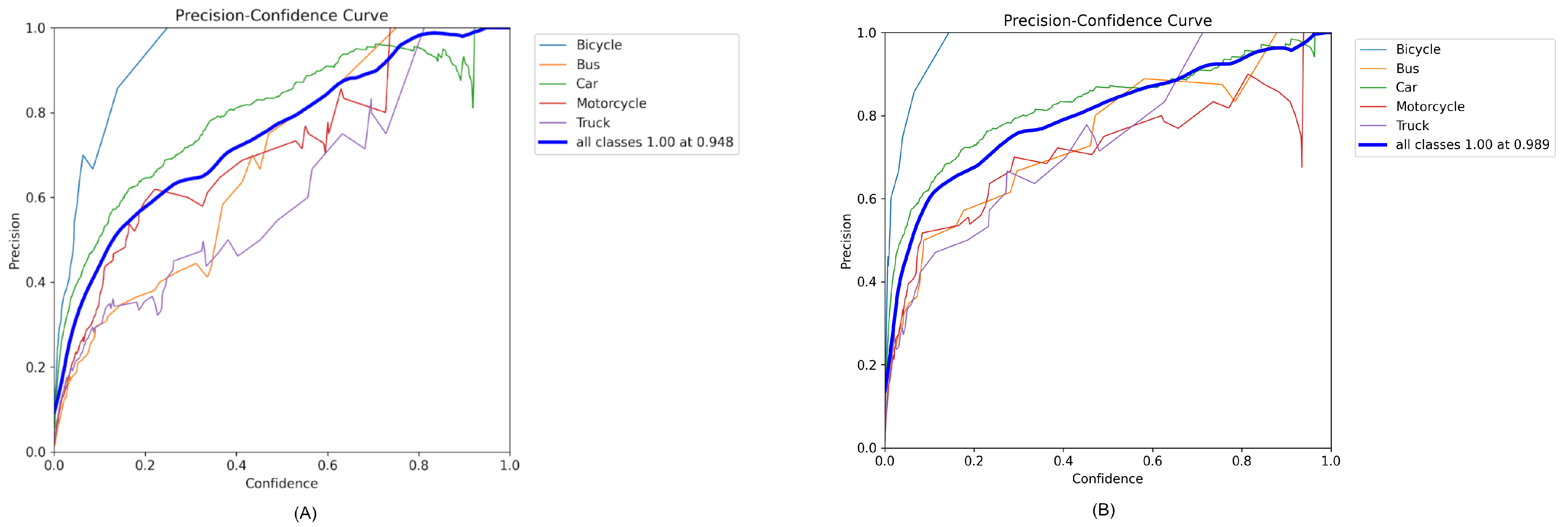
The precision–confidence curves for the YOLOv8 and YOLOv10 models, as displayed in Figure 5A,B, illustrate how the precision of vehicle detection varied with the confidence threshold for each class. These curves reveal a clear relationship between the confidence levels and the precision of detection for various vehicle classes, including bicycles, buses, cars, motorcycles, and trucks. As the confidence threshold increased, the precision of detecting each vehicle class generally increased, which reflects the models’ effectiveness in confidently predicting more accurate bounding boxes.
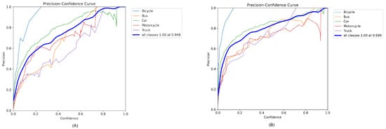
Figure 5.
Precision and confidence curve of (A) YOLOv8 and (B) YOLOv10.
In Figure 5A, representing YOLOv8, the precision for all classes combined approached a perfect score (1.00) at a confidence level of 0.948. This indicates the model’s excellent capability to accurately identify and classify objects when the confidence is high. Similarly, in Figure 5B for YOLOv10, the model achieved perfect precision (1.00) at an even higher confidence threshold of 0.989. This demonstrates the incremental improvements in the YOLOv10 model in handling detection with high confidence.
Specifically, the curve for the motorcycle class shows considerable fluctuations in precision at lower confidence levels but stabilizes and increases as the confidence level approaches the 0.6–0.8 range, highlighting a relative challenge in motorcycle detection compared with other vehicle types. On the other hand, the bus and truck categories maintained higher precision across a wider range of confidence levels, indicating robustness in detecting larger vehicle types.
These insights underscore the models’ reliability and precision across various vehicle categories at higher confidence levels, reflecting their robustness in practical applications where high confidence in detection is crucial.
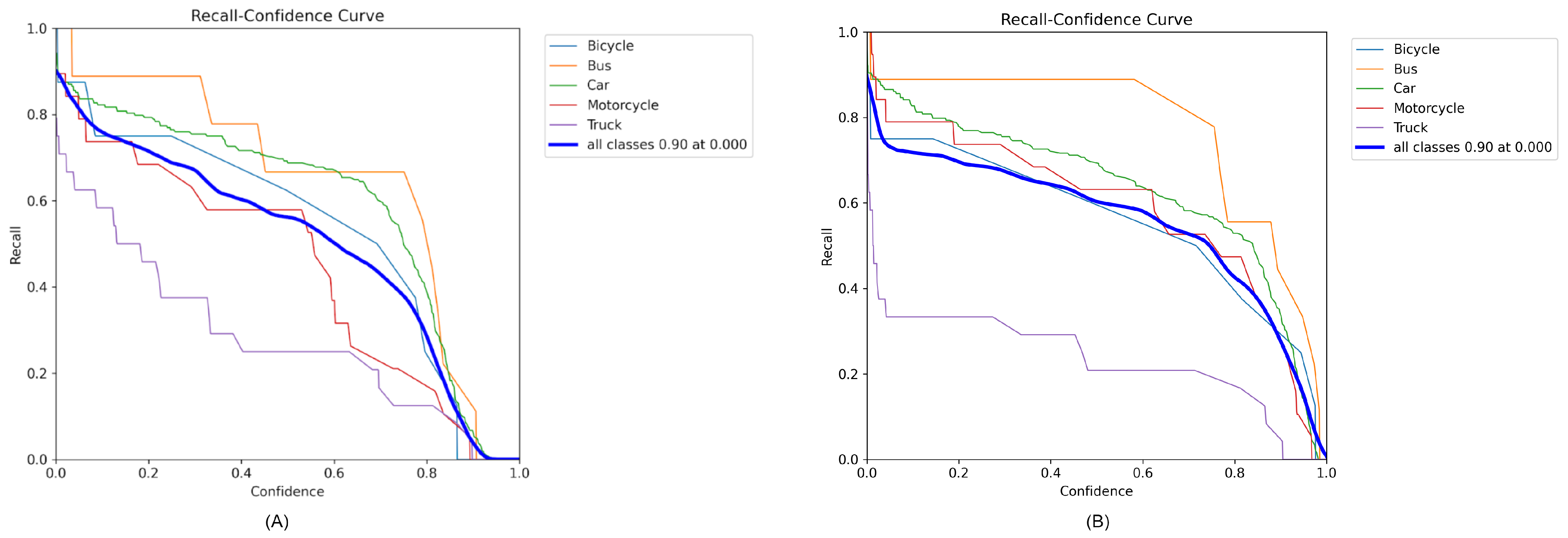
The recall–confidence curves for YOLOv8 and YOLOv10, as illustrated in Figure 6A,B, elucidate the trade-off between recall and confidence in the context of vehicle detection for various classes, such as bicycles, buses, cars, motorcycles, and trucks. The recall, which measures the proportion of actual positives correctly identified by the model, tended to decrease as the confidence threshold increased. This typical inverse relationship indicates that as the requirement for the model to be more confident in its predictions increases, the number of actual positives it detects tends to decrease.
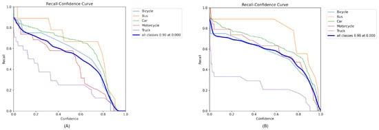
Figure 6.
Recall and confidence curves of (A) YOLOv8 and (B) YOLOv10 models.
In both graphs, the curves for different vehicle types show distinct behaviors, reflecting their varying detection challenges. For instance, the recall for motorcycles and trucks started relatively high at lower confidence levels, suggesting these models initially detected most of these vehicles but with varying degrees of confidence. As the confidence requirements increased, the recall for motorcycles and trucks sharply decreased, indicating fewer detections meeting the higher confidence threshold.
Notably, the curve representing all classes combined shows an initial high recall at extremely low confidence levels, achieving a recall of 0.90 at a confidence level of 0.000 in both YOLOv8 and YOLOv10. This demonstrates the models’ ability to detect a high number of actual positives initially, which declined as more stringent confidence thresholds were enforced.
Furthermore, the recall for cars and buses exhibited a more gradual decline compared with bicycles, which suggests that cars and buses are easier for the models to consistently detect across a range of confidence levels. Conversely, bicycles showed a steep drop in recall as the confidence level increased, highlighting specific challenges in detecting this class with high confidence.
These observations underscore the nuances of model performance across different vehicle classes, highlighting the balance between maintaining high recall and achieving high confidence in detections. This information is crucial for practical applications where missing detections (lower recall) can be critical, such as in autonomous driving and traffic monitoring systems.
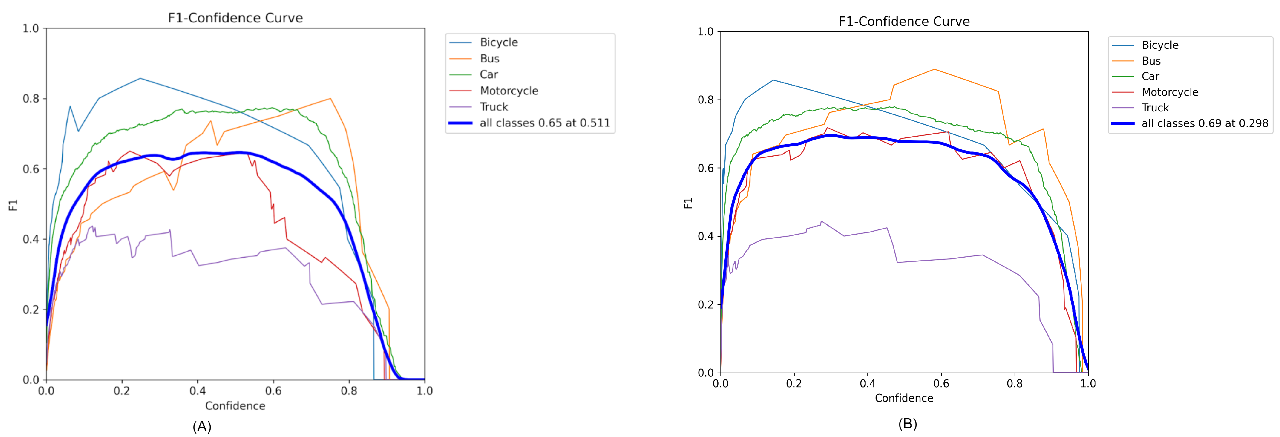
The F1–confidence curves for the YOLOv8 and YOLOv10 models, as shown in Figure 7A,B, depict the harmonic mean of the precision and recall at various confidence thresholds for different vehicle classes, including bicycles, buses, cars, motorcycles, and trucks. The F1 score serves as a balanced measure of the models’ precision and recall, providing a comprehensive metric of overall performance.
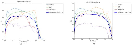
Figure 7.
F1 and confidence curves of (A) YOLOv8 and (B) YOLOv10 models.
For YOLOv8, the F1 score for all classes combined peaked at 0.65 at a confidence level of 0.511, indicating a balanced trade-off between recall and precision at this threshold. This peak suggests an optimal point for detecting objects across all classes with reasonable accuracy and minimal false negatives or positives. In contrast, YOLOv10 achieved a slightly higher peak F1 score of 0.69 at the same confidence level, reflecting improvements in either precision, recall, or both compared with YOLOv8.
When examining the curves in detail, YOLOv8 showed a steady increase in F1 score as the confidence level increased from zero, reaching a plateau around the 0.30–0.5 confidence range before gradually declining as the model became excessively strict in its predictions. On the other hand, YOLOv10 demonstrated a similar trend but maintained a higher F1 score across most confidence levels, indicating its enhanced ability to maintain high precision and recall simultaneously.
Specifically, the F1 scores for motorcycles and trucks in YOLOv10 exhibited higher peaks compared with those in YOLOv8, suggesting particular improvements in the detection of these vehicle types. Buses and cars also showed strong performance in both models but were particularly pronounced in YOLOv10, where the F1 curve remained above those for other vehicle classes across a broader range of confidence levels.
These curves clearly demonstrate the performance gains of YOLOv10 over YOLOv8, highlighting the former’s advanced capability in balancing detection accuracy across various vehicle categories at differing levels of confidence.
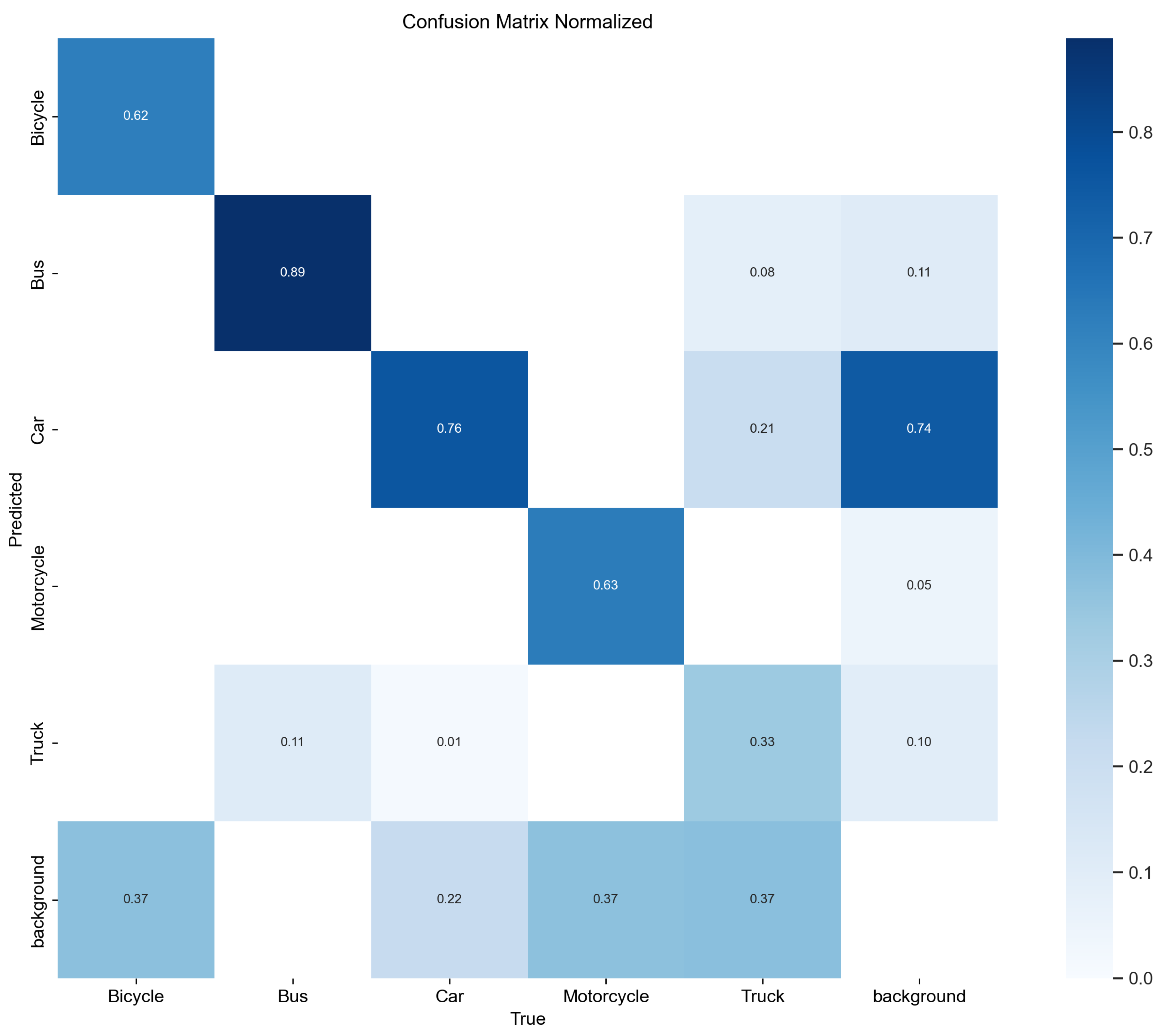
The normalized confusion matrices for YOLOv8 and YOLOv10 provide a clear comparative view of the classification accuracy across various vehicle classes, as depicted in Figure 8 and Figure 9. These matrices show the proportion of each class which was correctly classified, along with the distribution of misclassifications.

Figure 8.
Normalized confusion matrix for YOLOv8.
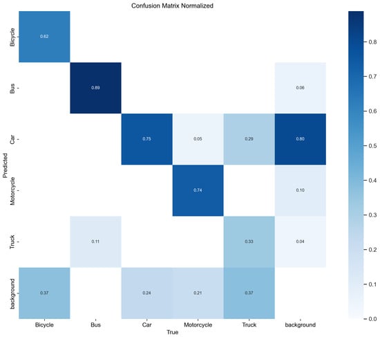
Figure 9.
Normalized confusion matrix for YOLOv10.
In Figure 8, YOLOv8 shows strong performance in correctly classifying buses with a high accuracy of 0.89, matching the performance seen in YOLOv10. For bicycles and trucks, both models achieved consistent, correct classification scores of 0.62 and 0.33, respectively. Notably, YOLOv8 slightly outperformed YOLOv10 in car classification with a score of 0.76, compared with 0.75 in YOLOv10, suggesting slightly better reliability in car detection.
However, YOLOv10, as shown in Figure 9, demonstrated a notable improvement in the classification of motorcycles, with a correct classification rate of 0.74 compared with 0.63 in YOLOv8. This improvement reflects enhancements in YOLOv10’s ability to handle the dynamic and smaller profile of motorcycles, which can be more challenging to detect accurately.
Both models also exhibited certain levels of misclassification, which were particularly noticeable where some motorcycles and trucks were misclassified as background pieces, which is highlighted by non-trivial values in the ‘background’ row of the confusion matrix. This might indicate challenges in distinguishing these vehicles from the background under certain conditions.
Additionally, the confusion matrices revealed areas where each model could potentially improve. For example, the lower scores in truck classification by both models suggest difficulties in distinguishing trucks from other vehicle types or the background, which could be due to their varied sizes and overlapping features with other large vehicles.
Overall, YOLOv10 shows a trend toward better overall accuracy, particularly in the challenging motorcycle category, while maintaining competitive performance in other categories when compared to YOLOv8.
5. Discussion
The comparative analysis between YOLOv8 and YOLOv10 for vehicle detection underscores the distinct performance characteristics inherent to each model. YOLOv10 demonstrated superior performance in detecting bicycles and trucks, with correct classification values of 0.87 and 0.33 compared with YOLOv8’s lower scores of 0.75 and 0.29, respectively. This enhancement suggests that YOLOv10 may incorporate optimizations and architectural improvements which are more adept at capturing the features of bicycles and trucks, possibly due to advanced feature extraction techniques or more effective handling of small or complex object geometries.
Conversely, YOLOv8 excelled in the detection of cars, achieving a higher classification accuracy of 0.82 against YOLOv10’s 0.79. This indicates that YOLOv8 may still retain certain advantages, particularly in recognizing features typical of passenger vehicles, which could stem from more targeted training or better tuning of model parameters for car-like shapes and sizes.
For the detection of buses and motorcycles, both models performed equivalently well, with each achieving a classification accuracy of 0.89 for buses and 0.74 for motorcycles. This parity in performance for these vehicle types suggests that the foundational elements of the YOLO architecture, present in both versions, are sufficiently robust for detecting these classes, indicating that either model may be effective in scenarios where buses and motorcycles are prevalent.
The observed discrepancies in model performance can be attributed to several factors. YOLOv10’s enhancements in handling bicycles and trucks may result from the incorporation of new layers or tuning strategies which improve the model’s ability to generalize from training data to real-world scenarios, particularly in handling objects with varying aspect ratios or in cluttered environments. On the other hand, the slight edge YOLOv8 holds in car detection could be linked to its potentially less complex but more focused approach to feature relevance, which may benefit the detection of more uniform and larger objects like cars.
These results suggest that YOLOv10 is generally more versatile, especially for detecting more challenging object classes such as bicycles and trucks, while YOLOv8 might be favored in applications where car detection is critical. Given the performance equivalency in detecting buses and motorcycles, the choice between these models could be determined by specific application needs, computational constraints, or the availability of training data.
Limitations of This Study
While this research provides a detailed comparative analysis of YOLOv8 and YOLOv10 in vehicle detection, there are several areas which were not explored and which can be addressed in future studies. Notably, the impact of varying environmental conditions, such as lighting and weather changes, on model performance was not assessed. Future research could investigate how these models perform under different scenarios, such as at nighttime or in adverse weather conditions, which are critical for real-world applications like autonomous driving. Additionally, this study did not examine the computational efficiency of the models in real-time processing environments, an important factor for deployment in onboard systems in vehicles. Further analysis may also include a deeper dive into the models’ performance on a larger and more diverse dataset which includes a wider variety of vehicle types and more complex urban scenarios. This would help in understanding the scalability and robustness of the models. Finally, integrating newer techniques, such as transfer learning or exploring the impact of different training strategies, might reveal additional insights into optimizing model performance for specific vehicle detection tasks.
In conclusion, the selection between YOLOv8 and YOLOv10 should consider these nuanced performance differences, aligning model capabilities with specific detection requirements and operational environments.
6. Conclusions
This research systematically compared the performance of the YOLOv8 and YOLOv10 models in the context of vehicle detection, highlighting the strengths and limitations of each model across different vehicle classes. The findings demonstrate that YOLOv10 generally offers improvements over YOLOv8, particularly in detecting bicycles and trucks, where it achieved higher classification accuracies. These enhancements likely stem from architectural advancements which enhance the model’s ability to capture complex features and handle objects with diverse shapes and sizes more effectively.
Conversely, YOLOv8 exhibited a slight advantage in car detection, suggesting that it remains effective for scenarios which predominantly involve passenger vehicles. Both models showed equivalent capabilities in detecting buses and motorcycles, indicating that the foundational features of the YOLO architecture robustly support the detection of these vehicle types.
Future Developments
Looking ahead, the field of vehicle detection using deep learning presents numerous avenues for further research and development. To address the practical demands of real-world applications, future studies could explore the impact of varied environmental conditions on model performance. This is particularly pertinent for applications requiring robust detection capabilities under different lighting and weather conditions [47].
Additionally, assessing the computational efficiency of these models in real-time environments would provide critical insights, especially for their potential integration into vehicle onboard systems. A broader evaluation employing a more diverse and extensive dataset would also be beneficial in assessing the scalability and robustness of these models.
Further exploration of advanced machine learning techniques, such as transfer learning, and experimentation with various training strategies could offer deeper insights into fine-tuning these models for specific vehicle detection tasks. Such advancements would not only refine the models but also expand the potential applications of the YOLO architecture in the field of autonomous driving and intelligent transportation systems, pushing the boundaries of current capabilities.
Author Contributions
Conceptualization, A.S.G.; methodology, A.S.G. and M.A.R.A.; software, M.A.R.A.; validation, M.A.R.A., A.S.G. and M.H.; formal analysis, M.A.R.A.; investigation, A.S.G.; resources, A.S.G.; data curation, A.S.G.; writing—original draft preparation, A.S.G.; writing—review and editing, P.A.; visualization, A.S.G.; supervision, M.H.; project administration, P.A. All authors have read and agreed to the published version of the manuscript.
Funding
This research received no external funding.
Data Availability Statement
Available on reasonable request.
Conflicts of Interest
The authors declare no conflicts of interest.
References
- Dodia, A.; Kumar, S. A comparison of yolo based vehicle detection algorithms. In Proceedings of the 2023 International Conference on Artificial Intelligence and Applications (ICAIA) Alliance Technology Conference (ATCON-1), Bangalore, India, 21–22 April 2023; pp. 1–6. [Google Scholar]
- Laopracha, N.; Sunat, K. Comparative study of computational time that HOG-based features used for vehicle detection. In Recent Advances in Information and Communication Technology 2017, Proceedings of the 13th International Conference on Computing and Information Technology (IC2IT), Bangkok, Thailand, 6–7 July 2017; Springer: Cham, Switzerland, 2018; pp. 275–284. [Google Scholar]
- Pyo, J.; Bang, J.; Jeong, Y. Front collision warning based on vehicle detection using CNN. In Proceedings of the 2016 International SoC Design Conference (ISOCC), Jeju, Republic of Korea, 23–26 October 2016; pp. 163–164. [Google Scholar]
- Kavitha, M.; Gayathri, R.; Polat, K.; Alhudhaif, A.; Alenezi, F. Performance evaluation of deep e-CNN with integrated spatial-spectral features in hyperspectral image classification. Measurement 2022, 191, 110760. [Google Scholar] [CrossRef]
- Ali, L.; Alnajjar, F.; Jassmi, H.A.; Gocho, M.; Khan, W.; Serhani, M.A. Performance evaluation of deep CNN-based crack detection and localization techniques for concrete structures. Sensors 2021, 21, 1688. [Google Scholar] [CrossRef] [PubMed]
- Girshick, R.; Donahue, J.; Darrell, T.; Malik, J. Rich feature hierarchies for accurate object detection and semantic segmentation. In Proceedings of the IEEE Conference on Computer Vision and Pattern Recognition, Columbus, OH, USA, 23–28 June 2014; pp. 580–587. [Google Scholar]
- Girshick, R. Fast r-cnn. In Proceedings of the IEEE International Conference on Computer Vision, Santiago, Chile, 7–13 December 2015; pp. 1440–1448. [Google Scholar]
- Gao, Y.; Guo, S.; Huang, K.; Chen, J.; Gong, Q.; Zou, Y.; Bai, T.; Overett, G. Scale optimization for full-image-CNN vehicle detection. In Proceedings of the 2017 IEEE Intelligent Vehicles Symposium (IV), Los Angeles, CA, USA, 11–14 June 2017; pp. 785–791. [Google Scholar]
- Dai, J.; Li, Y.; He, K.; Sun, J. R-Fcn: Object detection via region-based fully convolutional networks. Adv. Neural Inf. Process. Syst. 2016, 29. [Google Scholar]
- Alif, M.A.R.; Ahmed, S.; Hasan, M.A. Isolated Bangla handwritten character recognition with convolutional neural network. In Proceedings of the 2017 20th International Conference of Computer and Information Technology (ICCIT), Dhaka, Bangladesh, 22–24 December 2017; pp. 1–6. [Google Scholar]
- Azimjonov, J.; Özmen, A. A real-time vehicle detection and a novel vehicle tracking systems for estimating and monitoring traffic flow on highways. Adv. Eng. Inform. 2021, 50, 101393. [Google Scholar] [CrossRef]
- Zhang, S.; Wen, L.; Bian, X.; Lei, Z.; Li, S. Single-shot refinement neural network for object detection. arXiv 2017, arXiv:1711.06897. [Google Scholar]
- Fu, C.Y.; Liu, W.; Ranga, A.; Tyagi, A.; Berg, A.C. Dssd: Deconvolutional single shot detector. arXiv 2017, arXiv:1701.06659. [Google Scholar]
- Redmon, J.; Divvala, S.; Girshick, R.; Farhadi, A. You only look once: Unified, real-time object detection. In Proceedings of the IEEE Conference on Computer Vision and Pattern Recognition, Las Vegas, NV, USA, 27–30 June 2016; pp. 779–788. [Google Scholar]
- Redmon, J.; Farhadi, A. YOLO9000: Better, faster, stronger. In Proceedings of the IEEE Conference on Computer Vision and Pattern Recognition, Honolulu, HI, USA, 21–26 July 2017; pp. 7263–7271. [Google Scholar]
- Redmon, J.; Farhadi, A. Yolov3: An incremental improvement. arXiv 2018, arXiv:1804.02767. [Google Scholar]
- Bochkovskiy, A.; Wang, C.Y.; Liao, H.Y.M. Yolov4: Optimal speed and accuracy of object detection. arXiv 2020, arXiv:2004.10934. [Google Scholar]
- Li, C.; Li, L.; Jiang, H.; Weng, K.; Geng, Y.; Li, L.; Ke, Z.; Li, Q.; Cheng, M.; Nie, W. YOLOv6: A single-stage object detection framework for industrial applications. arXiv 2022, arXiv:2209.02976. [Google Scholar]
- Wang, C.Y.; Bochkovskiy, A.; Liao, H.Y.M. YOLOv7: Trainable bag-of-freebies sets new state-of-the-art for real-time object detectors. In Proceedings of the IEEE/CVF Conference on Computer Vision and Pattern Recognition, Vancouver, BC, Canada, 17–24 June 2023; pp. 7464–7475. [Google Scholar]
- Jocher, G.; Munawar, M.R.; Chaurasia, A. YOLO: A Brief History; 2023. Available online: https://www.scirp.org/reference/referencespapers?referenceid=3532980 (accessed on 11 February 2023).
- Al Rabbani Alif, M.; Hussain, M. YOLOv1 to YOLOv10: A comprehensive review of YOLO variants and their application in the agricultural domain. arXiv 2024, arXiv:2406.10139. [Google Scholar]
- Fernandez-Sanjurjo, M.; Bosquet, B.; Mucientes, M.; Brea, V.M. Real-time visual detection and tracking system for traffic monitoring. Eng. Appl. Artif. Intell. 2019, 85, 410–420. [Google Scholar] [CrossRef]
- Mandellos, N.A.; Keramitsoglou, I.; Kiranoudis, C.T. A background subtraction algorithm for detecting and tracking vehicles. Expert Syst. Appl. 2011, 38, 1619–1631. [Google Scholar] [CrossRef]
- Erbs, F.; Barth, A.; Franke, U. Moving vehicle detection by optimal segmentation of the dynamic stixel world. In Proceedings of the 2011 IEEE Intelligent Vehicles Symposium (IV), Baden-Baden, Germany, 5–9 June 2011; pp. 951–956. [Google Scholar]
- Ren, S.; He, K.; Girshick, R.; Sun, J. Faster R-CNN: Towards real-time object detection with region proposal networks. IEEE Trans. Pattern Anal. Mach. Intell. 2016, 39, 1137–1149. [Google Scholar] [CrossRef] [PubMed]
- Liu, W.; Anguelov, D.; Erhan, D.; Szegedy, C.; Reed, S.; Fu, C.Y.; Berg, A.C. Ssd: Single shot multibox detector. In Proceedings of the Computer Vision–ECCV 2016: 14th European Conference, Amsterdam, The Netherlands, 11–14 October 2016; Proceedings, Part I 14. Springer: Berlin/Heidelberg, Germany, 2016; pp. 21–37. [Google Scholar]
- He, K.; Zhang, X.; Ren, S.; Sun, J. Deep residual learning for image recognition. In Proceedings of the IEEE Conference on Computer Vision and Pattern Recognition, Las Vegas, NV, USA, 26 June–1 July 2016; pp. 770–778. [Google Scholar]
- Alif, M.A.R.; Hussain, M.; Tucker, G.; Iwnicki, S. BoltVision: A Comparative Analysis of CNN, CCT, and ViT in Achieving High Accuracy for Missing Bolt Classification in Train Components. Machines 2024, 12, 93. [Google Scholar] [CrossRef]
- Alif, M.A.R.; Hussain, M. Lightweight Convolutional Network with Integrated Attention Mechanism for Missing Bolt Detection in Railways. Metrology 2024, 4, 254–278. [Google Scholar] [CrossRef]
- Alif, M.A.R. Attention-Based Automated Pallet Racking Damage Detection. Int. J. Innov. Sci. Res. Technol. 2024, 9, 728–740. [Google Scholar]
- Hussain, M. YOLO-v5 Variant Selection Algorithm Coupled with Representative Augmentations for Modelling Production-Based Variance in Automated Lightweight Pallet Racking Inspection. Big Data Cogn. Comput. 2023, 7, 120. [Google Scholar] [CrossRef]
- Zahid, A.; Hussain, M.; Hill, R.; Al-Aqrabi, H. Lightweight convolutional network for automated photovoltaic defect detection. In Proceedings of the 2023 9th International Conference on Information Technology Trends (ITT), Dubai, United Arab Emirates, 24–25 May 2023; IEEE: New York, NY, USA, 2023; pp. 133–138. [Google Scholar]
- Alif, M.A.R. State-of-the-Art Bangla Handwritten Character Recognition Using a Modified Resnet-34 Architecture. Int. J. Innov. Sci. Res. Technol. 2024, 9, 438–448. [Google Scholar]
- Sang, J.; Wu, Z.; Guo, P.; Hu, H.; Xiang, H.; Zhang, Q.; Cai, B. An improved YOLOv2 for vehicle detection. Sensors 2018, 18, 4272. [Google Scholar] [CrossRef]
- Ćorović, A.; Ilić, V.; Ðurić, S.; Marijan, M.; Pavković, B. The real-time detection of traffic participants using YOLO algorithm. In Proceedings of the 2018 26th Telecommunications Forum (TELFOR), Belgrade, Serbia, 20–21 November 2018; pp. 1–4. [Google Scholar]
- Hu, X.; Wei, Z.; Zhou, W. A video streaming vehicle detection algorithm based on YOLOv4. In Proceedings of the 2021 IEEE 5th Advanced Information Technology, Electronic and Automation Control Conference (IAEAC), Chongqing, China, 12–14 March 2021; Volume 5, pp. 2081–2086. [Google Scholar]
- Kasper-Eulaers, M.; Hahn, N.; Berger, S.; Sebulonsen, T.; Myrland, Ø.; Kummervold, P.E. Detecting heavy goods vehicles in rest areas in winter conditions using YOLOv5. Algorithms 2021, 14, 114. [Google Scholar] [CrossRef]
- Li, C.; Li, L.; Geng, Y.; Jiang, H.; Cheng, M.; Zhang, B.; Ke, Z.; Xu, X.; Chu, X. Yolov6 v3. 0: A full-scale reloading. arXiv 2023, arXiv:2301.05586. [Google Scholar]
- Rouf, M.A.; Wu, Q.; Yu, X.; Iwahori, Y.; Wu, H.; Wang, A. Real-time vehicle detection, tracking and counting system based on YOLOv7. Embed. Selforganising Syst. 2023, 10, 4–8. [Google Scholar]
- Farid, A.; Hussain, F.; Khan, K.; Shahzad, M.; Khan, U.; Mahmood, Z. A fast and accurate real-time vehicle detection method using deep learning for unconstrained environments. Appl. Sci. 2023, 13, 3059. [Google Scholar] [CrossRef]
- Soylu, E.; Soylu, T. A performance comparison of YOLOv8 models for traffic sign detection in the Robotaxi-full scale autonomous vehicle competition. Multimed. Tools Appl. 2024, 83, 25005–25035. [Google Scholar] [CrossRef]
- Al Mudawi, N.; Qureshi, A.M.; Abdelhaq, M.; Alshahrani, A.; Alazeb, A.; Alonazi, M.; Algarni, A. Vehicle detection and classification via YOLOv8 and deep belief network over aerial image sequences. Sustainability 2023, 15, 14597. [Google Scholar] [CrossRef]
- Nielsen, N. Comparison between YOLOv10, YOLOv9 and YOLOv8 on Real-World Videos. 2024. Available online: https://www.youtube.com/watch?app=desktop&v=x20MxX-AWzE (accessed on 7 August 2024).
- Boneh, M. Vehicle-Detection. 2021. Available online: https://github.com/MaryamBoneh/Vehicle-Detection (accessed on 11 February 2023).
- Terven, J.; Córdova-Esparza, D.M.; Romero-González, J.A. A comprehensive review of yolo architectures in computer vision: From yolov1 to yolov8 and yolo-nas. Mach. Learn. Knowl. Extr. 2023, 5, 1680–1716. [Google Scholar] [CrossRef]
- Wang, A.; Chen, H.; Liu, L.; Chen, K.; Lin, Z.; Han, J.; Ding, G. Yolov10: Real-time end-to-end object detection. arXiv 2024, arXiv:2405.14458. [Google Scholar]
- Hussain, T.; Hussain, M.; Al-Aqrabi, H.; Alsboui, T.; Hill, R. A Review on Defect Detection of Electroluminescence-Based Photovoltaic Cell Surface Images Using Computer Vision. Energies 2023, 16, 4012. [Google Scholar] [CrossRef]


Disclaimer/Publisher’s Note: The statements, opinions and data contained in all publications are solely those of the individual author(s) and contributor(s) and not of MDPI and/or the editor(s). MDPI and/or the editor(s) disclaim responsibility for any injury to people or property resulting from any ideas, methods, instructions or products referred to in the content. |
© 2024 by the authors. Licensee MDPI, Basel, Switzerland. This article is an open access article distributed under the terms and conditions of the Creative Commons Attribution (CC BY) license (https://creativecommons.org/licenses/by/4.0/).