Broadband Microstrip Antenna for 5G Wireless Systems Operating at 28 GHz

Abstract

Communication systems have been driven towards the fifth generation (5G) due to the demands of compact, high speed, and large bandwidth systems. These types of radio communication systems require new and more efficient antenna designs. This article presents a new design solution of a broadband microstrip antenna intended for use in 5G systems. The proposed antenna has a central operating frequency of 28 GHz and can be used in the LMDS (local multipoint distribution service) frequency band. The dimensions of the antenna and its parameters have been calculated, simulated, and optimized using the FEKO software. The antenna has a compact structure with dimensions (6.2 × 8.4 × 1.57) mm. Rogers RT Duroid 5880 material was used as a substrate for the antenna construction, which has a dielectric coefficient of 2.2 and a thickness of 1.57 mm. The antenna described in the article is characterized by a low reflection coefficient of −22.51 dB, a high energy gain value of 3.6 dBi, a wide operating band of 5.57 GHz (19.89%), and high energy efficiency.

1. Introduction

The growing demand for telecommunications services is stimulating the development of new call-handling technologies. Each generation of mobile technologies has brought with it an increase in the data transmission speed along with improved connection quality and new functionalities. The fourth generation (4G) technology, which is currently in use, has been available worldwide since 2009. The fifth generation (5G) network will enable a number of new services, including those related to the Internet of Things (IoT) and the concept of smart cities. The new technology will make use of low, medium, and high frequency bands, all of which have their advantages and limitations. However, wide-scale deployment of a 5G network requires preparation of antenna infrastructure and implementation of new technological solutions. A significant number of antennas (apart from antennas used for mobile devices) will be to be installed inside buildings, especially public utility buildings, including stadiums, railway stations, and shopping centers. It should be noted, at this point, that antennas installed in locations close to crowds would be smaller than those used in current macrocell transmitters. This is a fundamental difference and a common misunderstanding in public discussion. In a traditional antenna system, the power is radiated according to the established spatial characteristics. Therefore, the area in which users can be located, is predefined. In contrast, the power in a 5G antenna is radiated directionally, and focused on individual users or groups of users. Antenna radiation directions can change almost automatically, to focus on mobile users [1,2,3].

In this article, we describe the design process and a model of a microstrip antenna designed in FEKO software by Altair. The antenna’s main assumption is its frequency of operation in the 28 GHz band, i.e., in one of the frequency bands designed for operation of the 5G system [4]. Other important assumptions for the antenna model include a small size and the widest possible bandwidth. The antenna design process has been optimized to minimize dimensions and weight, thereby enabling the use of the designed antenna in mobile terminals, as well as facilitating integration with electronic devices.

2. Characteristics of the 5G System

The 5G network makes use of new technological solutions to meet the growing requirements of users. As a result, the new system will be able to handle an increasing number of devices, and to satisfy higher quality thresholds required by modern applications. It is an evolution of the 4G networks of today, which incorporates technologies capable of handling the rapidly increasing amount of transmitted data and facilitating data exchange between an ever-growing number of IoT devices. As is typical for the introduction of any next-generation network, it is expected that until its coverage and functionality can match or surpass existing 4G networks, the 5G network will need to coexist with such [1].

In addition to the existing usage scenarios of mobile networks, three additional scenarios are planned for the emerging 5G network, all of which will be of particular importance to users and will distinguish the 5G network from previous generations.

The first new usage scenario is an enhanced mobile broadband (eMBB), which enables high-speed internet access (up to 1 Gbps) and will be the defining feature of this network as compared with existing networks, especially in the initial phase of its implementation. This advantage of the 5G system over legacy solutions will increase the efficiency and quality of communications in society. As an example, this will enable services based on the provision of high-resolution multimedia, attractive methods of communication (e.g., video, augmented and virtual reality), as well as smart city services (e.g., transmission of content from high-resolution cameras) [2,3].

The second use of 5G networks is based on massive machine type communications (mMTC), where 5G will be able to support a very large number of connections from low-power devices, referred to as the Internet of Things (IoT), to the mobile network. These devices asynchronously exchange data, using the mobile network to communicate. This scenario assumes support for a large number of device types, with the reservation that these devices will use the mobile network in an occasional manner, exchanging small volumes of data [5].

The third use is referred to as ultra-reliable low latency communications (URLLC), which be a technology providing a minimum (1 ms) latency for data exchange over a mobile network for critical applications (e.g., drone control). In previous generations of mobile networks, latency values were longer and amounted to about 100 milliseconds for 3G networks, with about 30 milliseconds in case of 4G (LTE—Long Term Evolution) network [6].

According to the current state of standardization of the 5G network, it is intended to operate in three frequency bands, i.e., low, medium, and high. The use case of a particular band depends on its characteristics, which include two factors in particular, i.e., radio signal propagation and capacity of spectrum resources. The first factor is related to the physical properties of electromagnetic waves and determines the obtainable radio transmission range in changing weather conditions and radio signal coverage in hard-to-reach areas (e.g., interiors of buildings). The second factor is associated with the available amount of RF bands in a given frequency range, which can be used by 5G networks. It should be noted that high bandwidths also require a wide radio band, which, being a limited resource, is subject to rationing, and its use must also take into account RF communication applications other than 5G networks, such as TV broadcasts, radio communication for home automation equipment, etc.

In a 5G system, the following three frequency bands are assumed to be used first [1,2]:

• From 694 to 790 MHz (700 MHz band);
• From 3400 to 3800 MHz (3.6 GHz band);
• From 27.50 to 28.35 GHz (28 GHz band).

The 700 MHz band is characterized by good signal propagation and relatively low attenuation (absorption of signal by various obstacles), which helps cover large areas. Thanks to these characteristics, this band can be used for mMTC services. However, the 700 MHz band alone would not be able to provide broadband internet access to mobile users (eMBB), as it does not allow the use of MIMO, which would increase the capacity of each cell site. However, it can be used together with the bands listed below, which have large spectral resources. This manner of operation improves signal transmission quality from the user to the base station (i.e., “upstream”) [7].

The 3.6 GHz band does allow the use of mMIMO (massive MIMO), while, at the same time, it constitutes a compromise between propagation and capacity in terms of spectral resources, especially when combined with the 700 MHz band, which would improve upward connectivity. This band would be used to build a coverage layer for eMBB services in several of the largest cities, including communication routes between these locations. This band can also be used to introduce services that requires reliable transmission and particularly low latency (URLLC) in applications requiring the transmission of particularly large amounts of data, such as high-resolution images for medical or navigation purposes [7].

The 28 GHz band is limited in its use, in particular, because of the requirements applied to transmission between the user and the base station (the “upstream” link). It can be used, for example, for broadband access points and picocell applications (cMTC/URLLC). This band, due to its large capacity and the possibility of allocating large spectrum resources, may also be considered for the provision of internet access via a fixed wireless access service [1,7].

3. Frequency Range for Local Multipoint Distribution Service

The technological solutions used in the 5G system eliminate the disadvantages of LTE. These solutions make use of very high frequencies (in a 28 GHz millimeter band) and beamforming techniques. In that, several clients within the range of the same base station can use a 1 Gbps internet connection.

The usefulness of the 28 GHz band is limited, in particular, because of requirements applying to transmission between the user and the base station (the “upstream” link). The 28 GHz frequency band has been made available by the Federal Communications Commission (FCC) by reallocating the local multipoint block distribution service (LMDS) A1, which is 850 MHz wide and lies between 27.50 and 28.35 GHz bands [8,9,10].

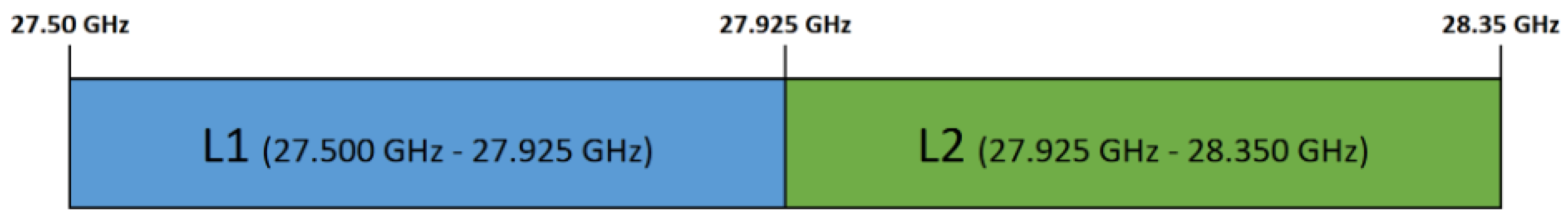
In response to the growing demand for an additional frequency spectrum, mostly for fixed/mobile 5G applications that require significant bandwidth to support higher speeds >1.0 Gbps at a lower latency, the Federal Communications Commission (FCC) has ordered the A1 channel and reallocated it as part of the new Upper Microwave Flexible Use License (UMFUS). The ordered part of the frequency spectrum has been transformed into a new licensing system based on two 425 MHz wide blocks (blocks L1 and L2) [10,11,12,13]. The division of the LMDS spectrum in the 28 GHz frequency band is presented in Figure 1.

The 28 GHz band and other millimeter frequency bands (mmWave), such as 24 GHz and 37/39 GHz bands, will play a key role in 5G implementations under the new Upper Microwave Flexible Use License (UMFUS). The UMFUS bands are standardized for 3GPP in accordance with 5G New Radio (NR) guidelines, in particular within Frequency Band 2 (FR2), which includes millimeter frequencies.

The UMFUS bands are currently maintained and used by national mobile phone operators, innovative mobile phone companies, regional phone operators, and other organizations wishing to implement mobile networks or provide fixed wireless access (FWA) services [8,9,10].

The UMFUS bands are subject to rules and regulations, which impose power limits at fixed and base stations operating in conjunction with mobile systems (EIRP density limit + 75 dBm/100 MHz). The average power of the sum of all antenna components in a mobile base station must not exceed a maximum EIRP value of +43 dBm. Network deployments may use any desired duplex scheme, provided that other technical or operational requirements are met [13].

The 28 GHz band is ideal for a wide range of applications making use of speeds >1 Gb/s (depending on channel size), which are achievable using the spectrum designated by UMFUS. High-speed backhaul, “at home” 5G/FWA, and other applications make use of the ability to implement fixed PTP (point-to-point) and PTMP (point-to-multi-point) configurations. The 28 GHz band can also be used for mobile applications, which are currently a key pillar of 5G deployment championed by national carriers and other organizations [11,12,13].

4. Analysis of Current Antenna Solutions Operating in 5G Systems at a 28 GHz Frequency

Current literature contains many proposed solutions of microstrip antennas operating in 5G systems at a frequency of 28 GHz [14,15,16,17,18,19,20,21,22,23]. These solutions are characterized by their compactness, small geometric dimensions, and antenna bandwidth of about 2 GHz. Many of them are based on a RT Duroid 5880 laminate with a permittivity of 2.2. In the analyzed antennas, the radiator is mostly rectangular, and is powered by a microstrip feed line. The proposed antenna is different, due to the modifications made to the shape of the patch, which were made on the basis of solutions originally used in fractal antennas. These modifications can be used to create a proposed antenna capable of supporting different bandwidths.

The antenna, proposed in this article, is capable of operating in systems intended for 5G communication, is designed for a resonance frequency equal to 28 GHz, and is based on a RT Duroid 5880 laminate with a rectangular radiator. The proposed antenna is designed to achieve a greater bandwidth than the antennas analyzed in the literature mentioned above. Antennas with a wider operating band can only be created by using complex spatial radiating structures, which makes them difficult to implement in 5G mobile devices.

The developed antenna, despite the use of the well-known inset feed in its design, has achieved a much wider bandwidth than similar constructions of this type found in the literature [14,15,16,17,18,19,20,21,22,23]. This effect was achieved through optimization with a large number of variables, which was aimed at achieving the lowest possible reflectance and voltage standing wave ratio (VSWR) in the widest possible frequency range. The results significantly exceed the previously published parameter values for this type of antenna in terms of bandwidth, especially in cases of strict matching conditions (VSWR ≤ 2, VSWR ≤ 1.5, and VSWR ≤ 1.25).

5. Broadband Microstrip Antenna Designed for Use in 5G Systems

The design process of a microstrip antenna consists of multiple stages. The main steps of the project process are presented below. The procedure for designing a single-piece rectangular microstrip antenna are the following:

• Determine operational frequency;
• Determine operational bandwidth;
• Choose a substrate;
• Choose substrate height;
• Determine the dimensions of the patch;
• Determine the power supply;
• Determine the electrical parameters and characteristics of the antenna;
• Optimize the antenna to obtain the best possible parameters in the given frequency range.

Before the development of a proper numerical model of the designed antenna could begin, it was necessary to perform preliminary calculations of its geometric parameters. These calculations were done to work out an approximate shape of the antenna, which would ensure that the structure complied with the assumptions adopted for its design. The dimensions of the individual edges of the antenna depend primarily on the resonance frequency, f_r, and the relative permittivity, ε_r, of the dielectric layer of the copper laminate, which are the foundation of the new antenna [24].

The antenna is designed to operate in a 5G system, on frequencies ranging from 27.50 GHz to 28.35 GHz (LMDS band) and the center frequency f_r = 28.00 GHz. Choosing the thickness of the substrate is one of the most important stages in the antenna design process, as the thickness of the substrate directly affects the efficiency and bandwidth of the microstrip antenna. One of the assumptions for this antenna is to obtain the widest bandwidth possible. As the thickness of the substrate increases, the antenna’s bandwidth increases, while its efficiency decreases. The upper value of the substrate thickness was determined from the following relationship [14,15]:

$$h\le \frac{0.3c}{2\pi f\sqrt{{\epsilon }_r}}\le \frac{0.3\times 3\times {10}^8}{2\pi \times 28\times {10}^9\sqrt{2.2}}\le \frac{90\times {10}^7}{260.8\times {10}^9}\le 3.45 \mathrm{mm}.$$

(1)

Taking into account the result provided above, the RT Duroid 5880 laminate was selected as a substrate, with a thickness of h = 1.57 mm, permittivity ε_r = 2.2, and tanδ = 9.0 × 10⁻⁴. In the next calculation step, the width of the radiating element should be determined from the following relationship [16,17]:

$$W=\frac{c}{2f_r}\sqrt{\frac{2}{{\epsilon }_r+1}}=\frac{3\times {10}^8}{2\times 28\times {10}^9}\sqrt{\frac{2}{2.2+1}=}4.17 \mathrm{mm}.$$

(2)

To determine the length of the radiating element, the effective permittivity ε_reff, of the substrate must first be calculated. It is defined by the following relationship [18,19]:

$${\epsilon }_{reff}=\frac{{\epsilon }_r+1}{2}+\frac{{\epsilon }_r-1}{2\sqrt{1+12\frac{h}{W}}}=\frac{2.2+1}{2}+\frac{2.2-1}{2\sqrt{1+12\times \frac{1.57}{4.17}}}=1.6+0.21=1.81.$$

(3)

Upon calculating ε_reff, the effective length of the patch Le should be determined from the following relationship [20,21]:

$$L_e=\frac{c}{2f_r\sqrt{{\epsilon }_{reff}}}=\frac{3\times {10}^8}{2\times 28\times {10}^9\sqrt{1.81}}=3.98 \mathrm{mm}.$$

(4)

Then, we calculate by how much the patch should be shortened using the following relationship [22,25]:

$$\Delta L=\frac{0.412\times h\left({\epsilon }_{reff}+0.3\right)\left(\frac{W}{h}+0.264\right)}{\left({\epsilon }_{reff}-0.258\right)\left(\frac{W}{h}+0.8\right)}=\frac{0.412\times 1.57\left(1.81+0.3\right)\left(\frac{4.17}{1.57}+0.264\right)}{\left(1.81-0.258\right)\left(\frac{4.17}{1.57}+0.8\right)}=0.74 \mathrm{mm}.$$

(5)

The final patch length value is:

$$L=L_e-2\Delta L=3.98-2\times 0.74=2.58 \mathrm{mm}.$$

(6)

Once the size of the radiating element is determined, the size of the reference plane also needs to be determined. The size of the reference plane is assumed to be greater than the radiating element by approximately six thicknesses of the substrate, by both width and length. The dimensions of the reference plane are determined by the following relationship [26,27]:

$$L_s=L+6h=2.58+6\times 1.57=12 \mathrm{mm}.$$

(7)

$$W_s=W+6h=4.17+6\times 1.57=13.59 \mathrm{mm}.$$

(8)

In the next step, we determine the inset feed gap from the following relation [21]:

$$f_{gap}=\frac{4.65\times {10}^{-18}·c·f_r}{\sqrt{2{\epsilon }_{reff}}}=\frac{4.65\times {10}^{-18}\times 3\times {10}^5\times 28\times {10}^9}{\sqrt{2\times 1.81}}=0.21 \mathrm{mm}.$$

(9)

The last step of the numerical antenna design process is to determine the size of the feed line. By calculating the dimensions of a microstrip feed line with a characteristic impedance Z_C = 50 Ω, we start the determination of auxiliary variables a and b as:

$$\begin{gathered} a=\frac{Z_c}{60}\sqrt{\frac{{\epsilon }_r+1}{2}}+\frac{{\epsilon }_r-1}{{\epsilon }_r+1}\left(0.23+\frac{0.11}{{\epsilon }_r}\right)=1.158 \\ b=\frac{60{\pi }^2}{Z_c\sqrt{{\epsilon }_r}}=7.97 \end{gathered}$$

(10)

Since parameter a is less than 1.52, the width and length of the feed line is determined from the following relationships [21,23]:

$$\begin{gathered} W_f=\frac{2}{\pi }\left\{b-1-ln\left(2b-1\right)+\frac{{\epsilon }_r-1}{2{\epsilon }_r}\left[ln\left(b-1\right)+0.39-\frac{0.61}{{\epsilon }_r}\right]\right\}·h \\ =3.07 \mathrm{mm}. \end{gathered}$$

(11)

$$L_f=3·h=3\times 1.57=4.71 \mathrm{mm}.$$

(12)

At this stage, the process of developing a numerical model of the designed antenna is complete. The calculations above resulted in the antenna dimensions presented in

Table 1. Dimensions of the preliminary antenna design.

Antenna Component	Symbol	Dimensions (mm)
Ground plane width	Ws = We	13.59
Ground plane length	Ls = Le	12.00
Patch width	Wp	4.17
Patch length	Lp	2.58
Copper thickness	Cu	0.05
Substrate thickness	h	1.57
Permittivity	Er	2.20
Feed line width	Wf	3.07
Feed line length	Lf	4.71

. The design of the developed antenna, as calculated, is shown in Figure 2. These data are be used to optimize the antenna in terms of bandwidth and miniaturize its dimensions.

6. Optimization Process and Discussion of Simulation Results

Computer simulations can help to determine the electrical parameters and radial characteristics of the antenna; in this case, we used FEKO software developed by the Altair company.

The analysis of electrical parameters of the radiating element design solution and other antenna elements indicates that there is room to improve the electrical parameters of the antenna by reducing VSWR, increasing the width of the operating band, miniaturizing antenna dimensions, and increasing antenna gain. For this purpose, the design was optimized for the parameters mentioned above, using FEKO software from the Altair company. The calculated parameters of the rectangular patch were used to create a preliminary simulation of the electrical parameters of the developed antenna model. Then, the model underwent a process of optimization, with the main assumption that the antenna must operate at the resonance frequency of 28 GHz.

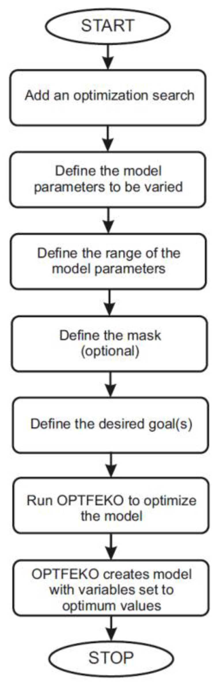
The FEKO software supports the ability to define the electrical parameters optimization process for the designed antenna and provides a number of options related to optimization. The algorithm of the optimization process used by the FEKO software is shown in Figure 3.

During the optimization process, one of the following optimization methods of FEKO software must be chosen: simplex (Nelder–Mead), particle swarm optimization (PSO), or genetic algorithm (GA). For the above methods, there are two options for stop criteria:

Specify maximum number of runs by the solver: The optimization process ends when the FEKO solver has been run a certain number of times during the optimization process. In the case of PSO and GA methods, if a full swarm or generation is not generated within the allowed number of assigned runs, optimization may be completed before the indicated number of runs by the solver. If the optimization process is terminated prematurely, due to a reduction in the number of runs by the solver, the software will provide the optimal solutions found up to that point, as well as information about the optimization process.

Optimization convergence accuracy (standard deviation): This option allows adjustment of accuracy levels required for the optimization process. Three options for selecting the accuracy level are available, i.e., high, normal, and low. The selected accuracy level of the optimization process modifies the conditions in which the search algorithm will converge, and the effect depends on the selected method.

In the optimization process of the proposed antenna, the option “specify maximum number of runs by the solver” was chosen. In the next step, we have to define the parameters of the antenna model that are to be changed during the optimization process in order to achieve an optimal solution. The parameters define the variables, which can be changed during the optimization process. These parameters are local for each optimization search, and a correct search must contain at least one defined parameter. Any variable defined in the FEKO software can be used as an optimization parameter, for example, the physical dimensions of the model, load, and source (amplitude and phase), provided that no relationship is implied between the optimization parameters in the same search.

During the optimization process, the length and width of the antenna base with the screen (W_s, W_e, L_s, and L_e), the length and width of the radiator (L_p and W_p), the length and width of the power line (L_f and W_f) and the length and width of the patch inset (Y₀ and X₀) were changed. Other structural elements, such as thickness and permittivity of the substrate, were not changed [28,29,30,31].

In the next step, we define the range of parameters to be changed, specifying their minimum, maximum, and initial values. For each optimization parameter, a minimum value and a maximum value must be defined, and optionally, an initial value can be given as well. The initial value will influence the optimization process when using particle swarm optimization or genetic algorithm. If the starting value is not specified by the user, the value in the middle of the range of the parameter will be taken as the starting point of the optimization. In our optimization process, we selected the minimum, maximum, and start values based on calculated parameters of the rectangular patch and the center frequency.

In the next step, we define an optimization mask. An optimization mask is a set of user-defined values forming a continuous line. The mask is a criterion to which the optimal solution must adhere. It is specified that the optimized solution is smaller, equal, or larger than the mask. When calculating an optimal solution, the target values are compared with the mask. If the mask criterion is met, the values are added to the value table. We do not define an optimization mask in our optimization process.

The last step of the optimization process is the selection of the optimization target. The objectives, which need to be defined, specify the desired state that the optimization process should try to achieve by changing certain parameters of the antenna model.

For each optimization search, goals should be defined to determine the desired state that the optimization process should aim to achieve. Many goals can be defined, but a correct optimization search must include at least one goal. During the optimization process we define the following goals:

• Impedance goal (input impedance, input admittance, reflection coefficient (S₁₁), transmission coefficient, VSWR, return losses, current);
• Near-field goal (E field – electric field, H field – magnetic field, directional component, coordinate system);
• Far-field goal (E field, antenna gain, directivity, RCS – Radar Cross Section);
• S-parameter goal (coupling coefficient, reflection coefficient, transmission coefficient, VSWR, return losses);
• SAR (Specific Absorption Rate) goal;
• Power goal (efficiency, active power, power loss);
• Transmission/reflection coefficients goal (reflection, transmission, co-polarization, and cross-polarization);
• Receiving antenna power goal (efficiency, active power, and power loss).

In our optimization process, we chose an impedance target (reflectance and VSWR) with a target minimization operator. The impedance target provides optimization related to the impedance and admittance of any voltage or current source, which is solved within the FEKO model. The reflectance ratio is calculated in relation to the indicated reference impedance.

In the case of an impedance target, the reflection factor is calculated directly from the observed input impedance. Therefore, this value is the active reflection factor, and may differ from the S₁₁, which was calculated during the calculation of the S parameter in the multiport model. The voltage standing waveform factor for the observed input impedance is considered in relation to the indicated reference impedance.

Once the parameters of the optimization process have been defined, we can run “OPTFEKO” to calculate the optimal solution for the specified parameters. Once the optimal values for the model are obtained, the FEKO model with the optimal parameters is created.

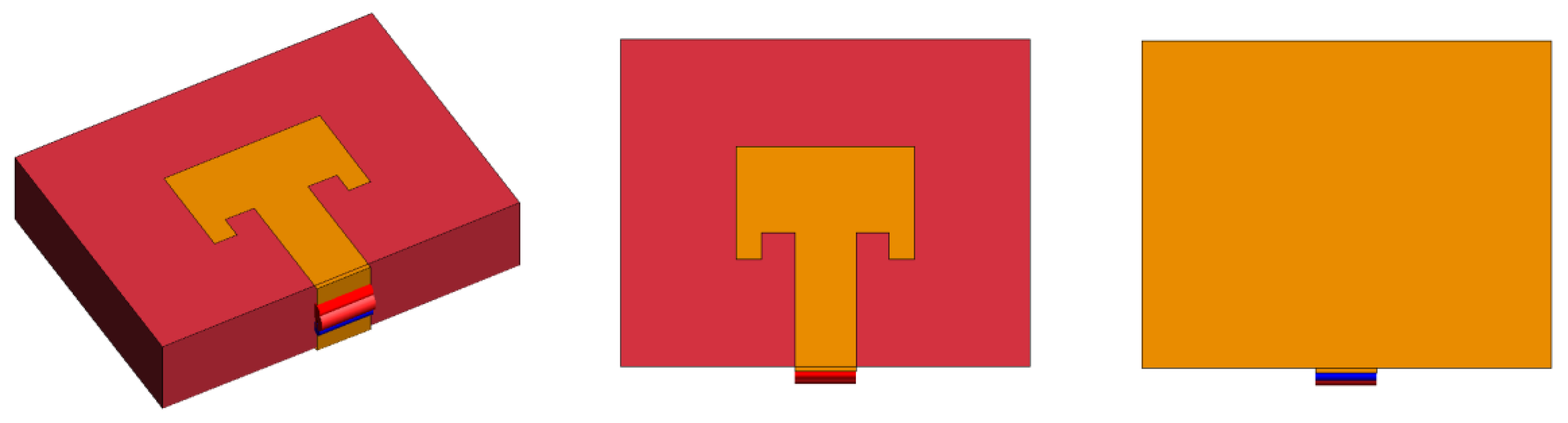
The optimization process resulted in a final design of the antenna model, as shown in Figure 4. Dimensions of this design are shown in

Table 2. Dimensions of the optimized antenna model.

Antenna Component	Symbol	Dimensions (mm)
Ground plane width	Ws = We	8.40
Ground plane length	Ls = Le	6.20
Patch width	Wp	3.66
Patch length	Lp	2.14
Copper thickness	Cu	0.05
Substrate thickness	h	1.57
Permittivity	Er	2.2
Feed line width	Wf	1.26
Feed line length	Lf	3.10
Inset feed gap	Y0	0.50
Width feed gap	X0	0.68

.

The resulting antenna design was simulated with the use of FEKO software from the Altair company, which provided results for the following electrical parameters: reflection coefficient, standing wave ratio, input impedance, antenna gain, current distribution in the antenna, and radiation characteristics.

6.1. Q Factor

The Q factor of an antenna is defined in the same way as for resonant circuits, i.e., the ratio of energy stored to energy lost during one period of vibration. The difference is in the user’s expectations, while for resonant circuits, a high Q factor is usually required, the opposite is true for antennas. By determining the Q factor, it is possible to easily estimate the bandwidth of an antenna. The larger BW is because of a reduction in the Q factor of the patch resonator, which is due to less energy being stored beneath the patch, and due to higher radiation. In order to determine the Q factor value in the first step, we analytically determine the bandwidth of the antenna based on the dimensions of the proposed antenna model (dimensions of the radiating element and the thickness of the substrate), using the following dependencies:

$$\begin{gathered} BW=3.771·\left[\frac{{\epsilon }_r-1}{{\left({\epsilon }_r\right)}^2}\right]·\frac{h}{{\lambda }_0}·\left(\frac{W}{L}\right)=3.771\times \left[\frac{2.2-1}{{2.2}^2}\right]\times \frac{1.57}{10.7 }\times \left(\frac{3.66}{2.14}\right) \\ =3.771\left[\frac{1.2}{4.84}\right]\times 0.146728\times 1.71028=23\% \end{gathered}$$

(13)

The theoretical bandwidth for the antenna, calculated from mathematical relationships, is about 23%. The BW of the microstrip antenna is inversely proportional to its Q factor and is given by [32] the following:

$$BW=\frac{\left(VSWR-1\right)}{Q\sqrt{VSWR}}$$

(14)

Having determined the theoretical bandwidth BW and taking VSWR = 2 as the limit value for the bandwidth, after transforming the above Relation (14) the Q factor of the antenna was determined as:

$$Q=\frac{\left(VSWR-1\right)}{BW\sqrt{VSWR}}=\frac{\left(2-1\right)}{0.23\sqrt{2}}=\frac{1}{0.3252}=3.07.$$

(15)

The analytically low value of the antenna’s Q factor confirms its ability to operate in a wide frequency range.

6.2. Reflection Coefficient

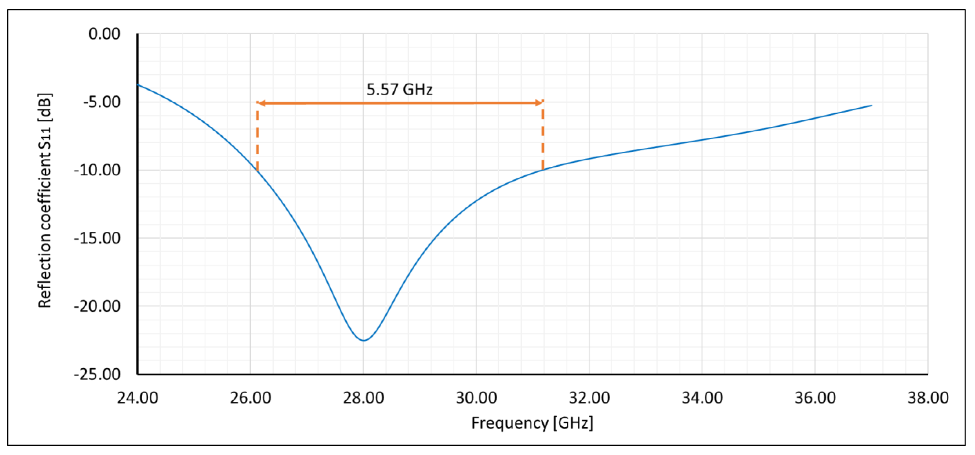
The base value of the reflection coefficient is assumed to be −10 dB, which means that 10% of the incident power is reflected, i.e., 90% of the power is received by the antenna, which is considered to be perfect for mobile communication [24,33]. The proposed antenna has a resonance at 28.00 GHz with a reflection loss of −22.50 dB, as shown in Figure 5. The S₁₁ parameter was obtained by powering the antenna using the edge port. The antenna has an operating bandwidth of 5.57 GHz, which gives a relative operating bandwidth of 19.89%. The bandwidth determined from the results of computer simulations is slightly smaller than the theoretical bandwidth determined on the basis of Relation (13), due to the inset feed used as a power supply. Nevertheless, this method of supplying power to a microstrip antenna provides us with better impedance matching (lower reflection factor value) for a resonance frequency.

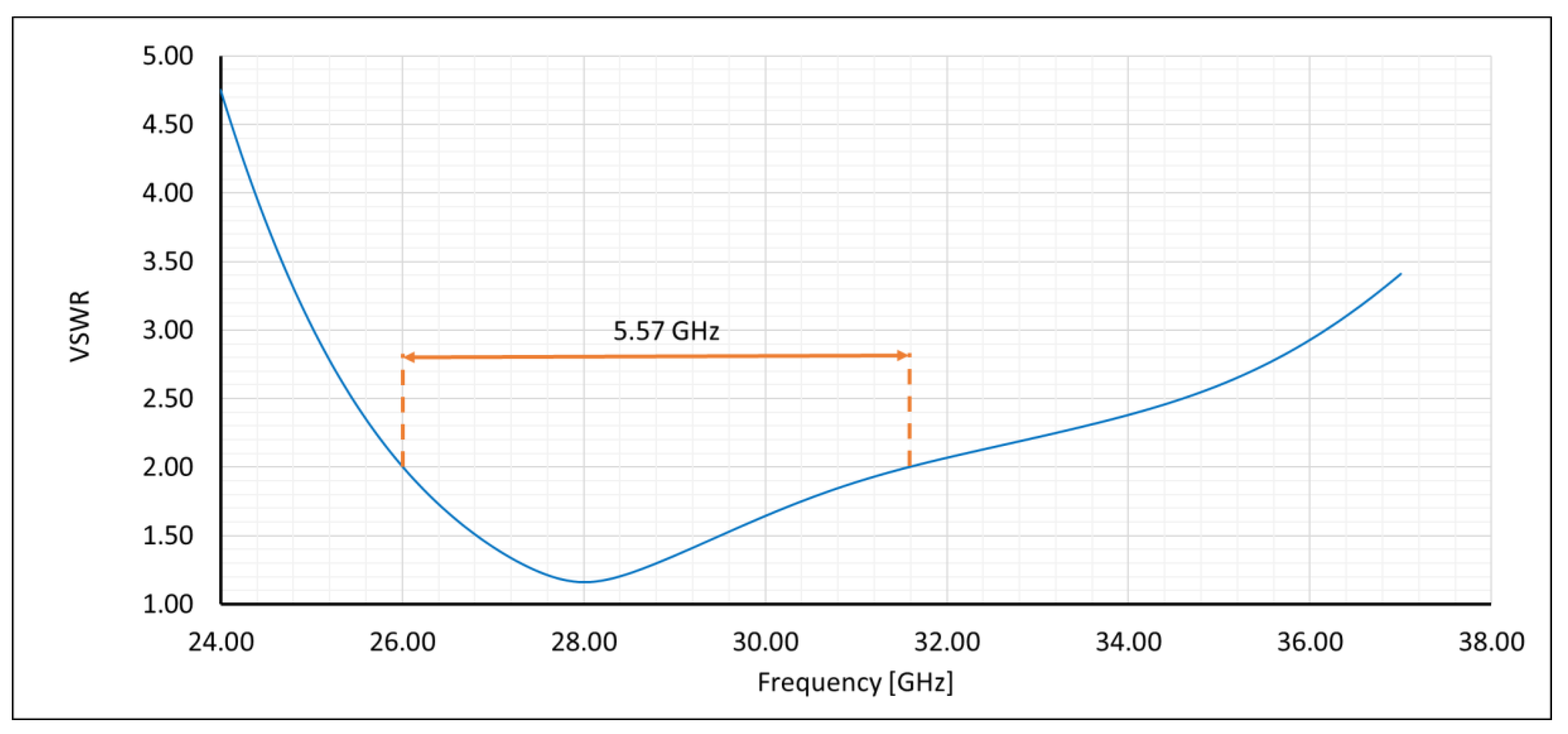
6.3. Voltage Standing Wave Ratio

In the case of a patch antenna, the voltage standing wave ratio (VSWR) should not be greater than 2 across the entire frequency band. Ideally, this value should equal 1 [24,34]. The voltage standing wave ratio as a function of frequency is shown in Figure 6. As can be seen in Figure 6, the VSWR value obtained at a resonance frequency of 28.00 GHz equals 1.162, and the VSWR value of 2 was determined at 26.01 and 31.58 GHz respectively. The above values show that the proposed antenna operates in the whole assumed frequency band (LMDS), i.e., from 27.50 to 28.35 GHz.

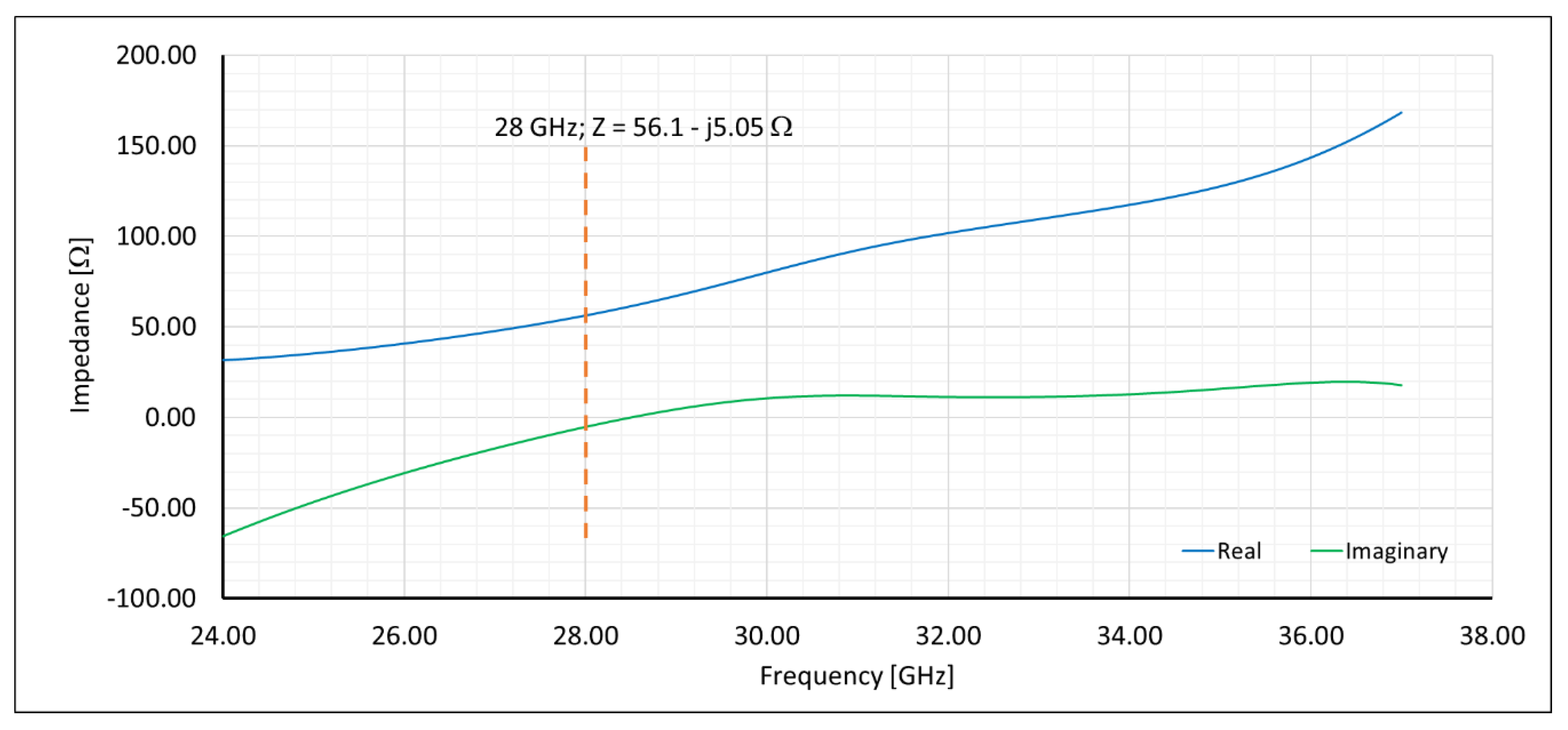
6.4. Input Impedance

The antenna’s design assumes that the impedance of the power line should be 50 Ω. In the case of large discrepancies, it is possible to use a matching system. However, adding another system introduces additional losses and generates additional costs [35,36,37]. The designed width and length of the feed line in the antenna has a complex input impedance of Z = 56.1 + j5.08 Ω at the resonance frequency of 28.00 GHz, while at 27.50 GHz the complex input impedance is Z = 51.57 − j10.73 Ω, and at 28.35 GHz the complex input impedance is Z = 59.6 − j1.39 Ω. Detailed input impedance values for the proposed antenna as a function of frequency are shown in Figure 7.

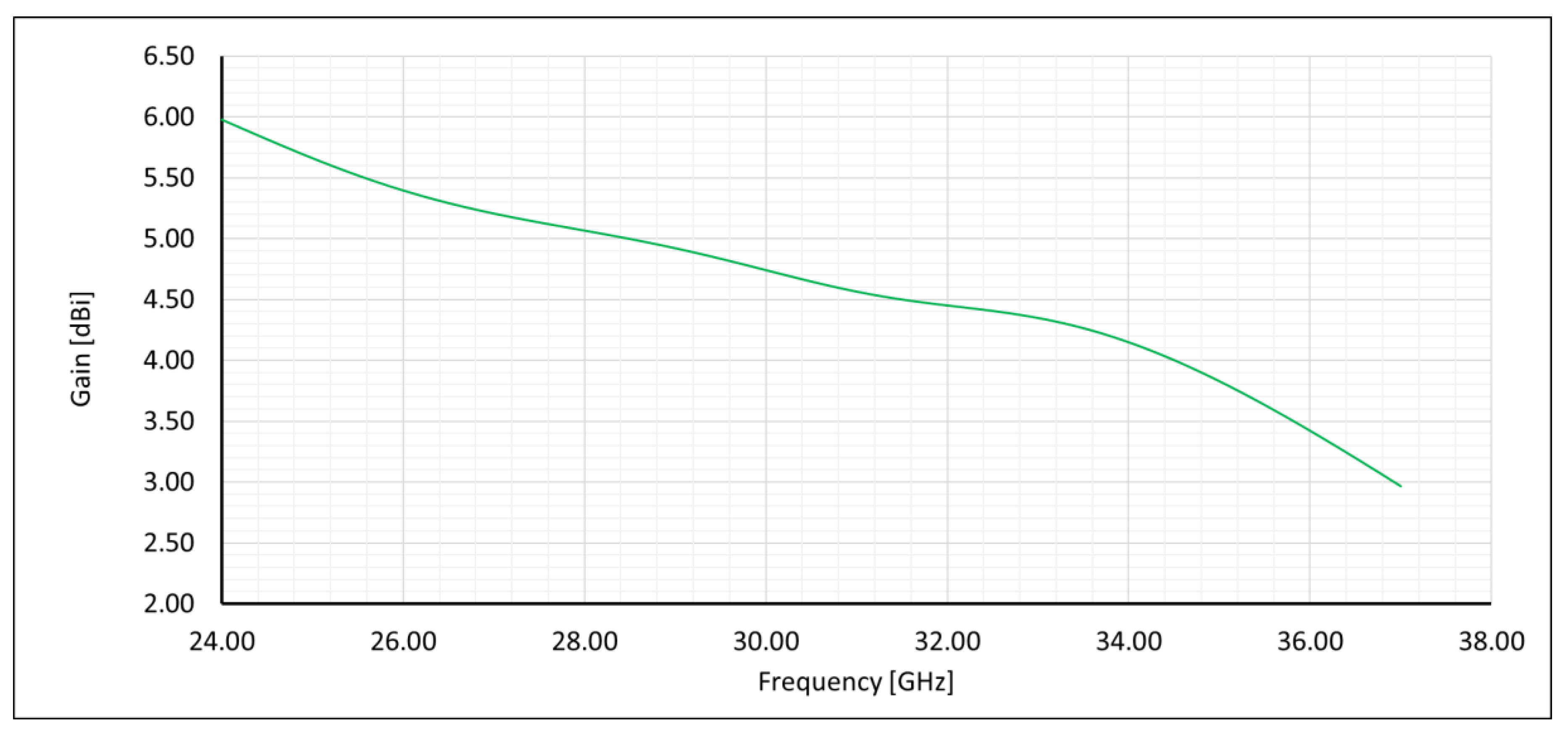
6.5. Antenna Gain

Usually, antenna gain is given in relation to an isotropic antenna and is expressed in dBi. In some cases, antenna gain is also given in relation to the dipole antenna and expressed in dBd. The energy gain of an antenna is dependent on its directivity and the energy loss of the antenna, which results from the material it is made of [35,37]. The proposed antenna has a gain of 5.06 dBi at a resonance frequency of 28.00 GHz, which is considered to be high for compact microstrip antennas. Values of antenna gain as a function of frequency are shown in Figure 8.

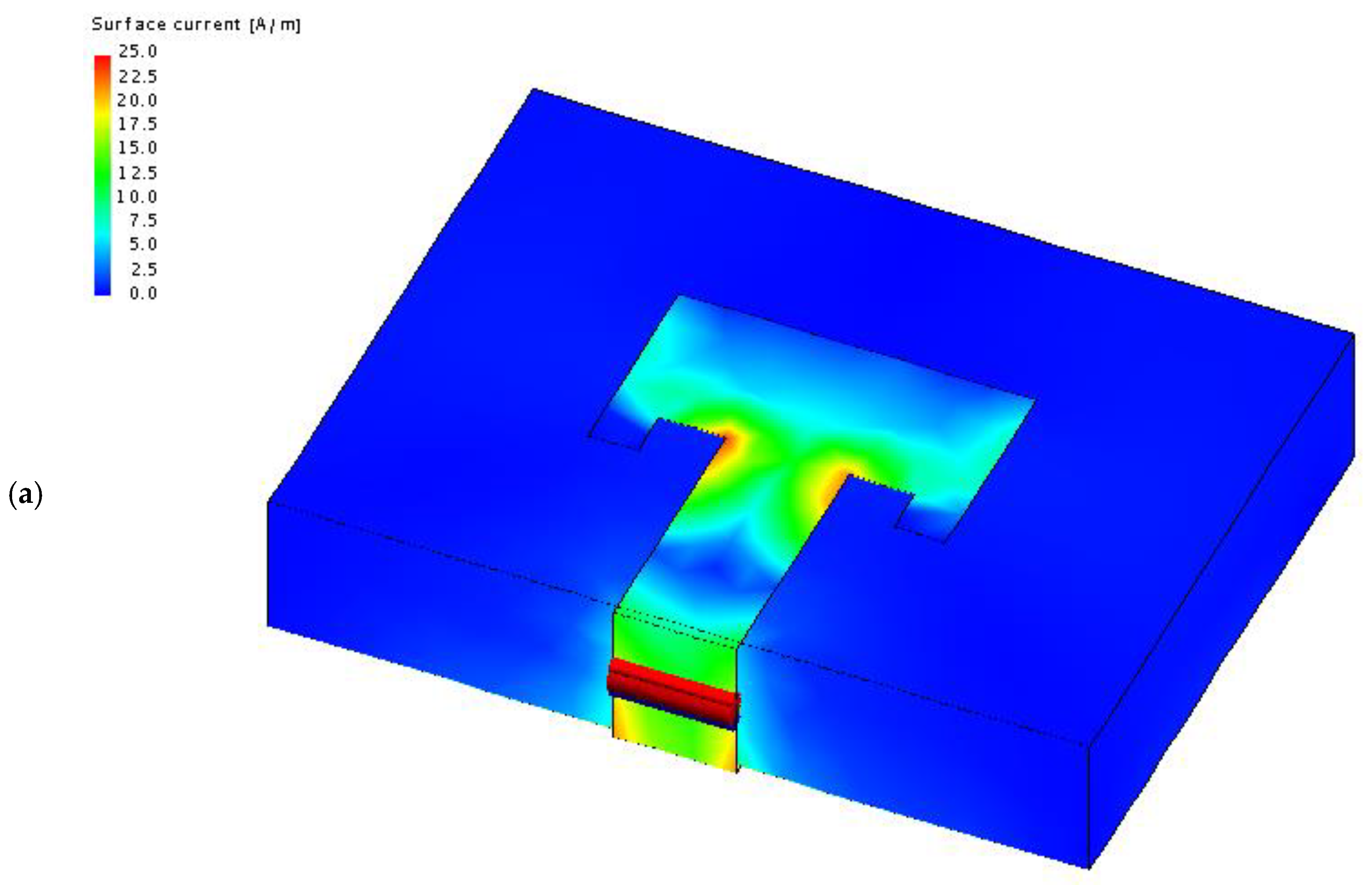
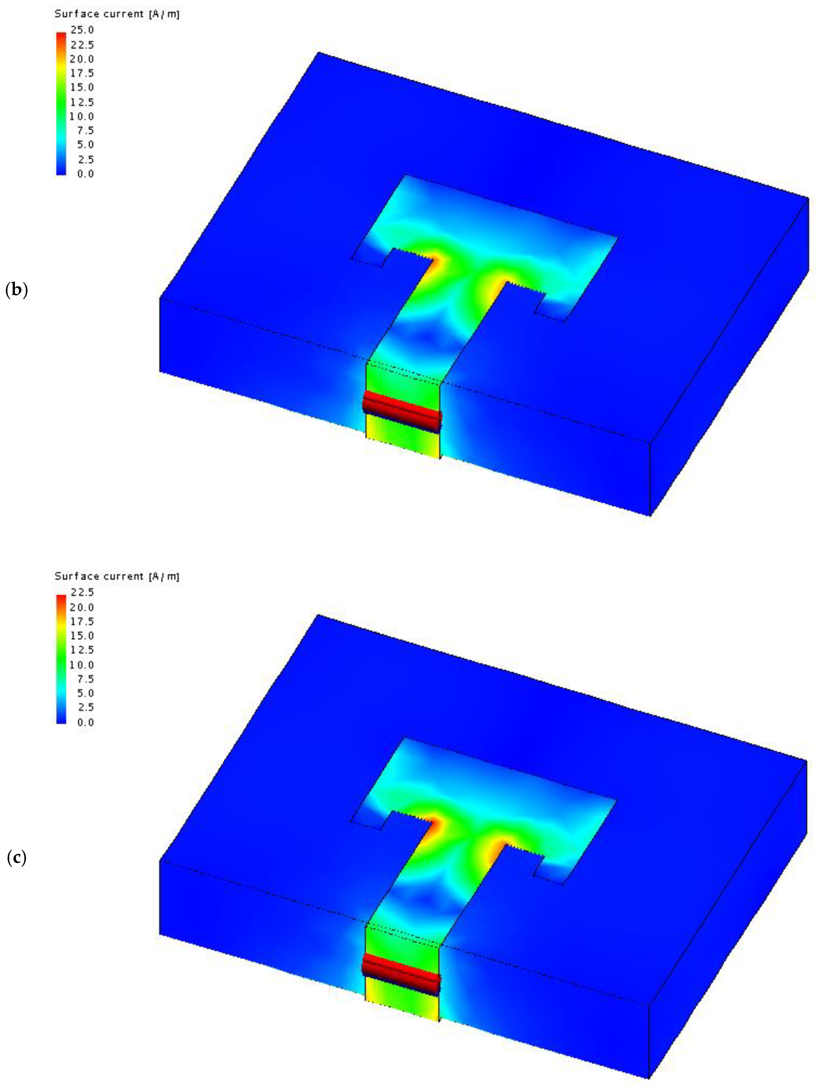
6.6. Current Distribution in the Antenna

In a microstrip antenna, the value of the current should be minimal at the end of the radiating element (the edge of the patch). The voltage at the edge of the patch is phase shifted in relation to the current. Therefore, peak voltage is present at the end of the patch, with current values close to zero [33,37]. A similar situation occurs in the middle of the wave, further down the line, i.e., at the beginning of the patch. The phase-shifted voltage in relation to the current phase produces fields on the edges of a microstrip antenna. The current distribution of the developed antenna at frequencies of 27.51 GHz (a), 28.0 GHz (b), and 28.35 GHz (c) is presented in Figure 9.

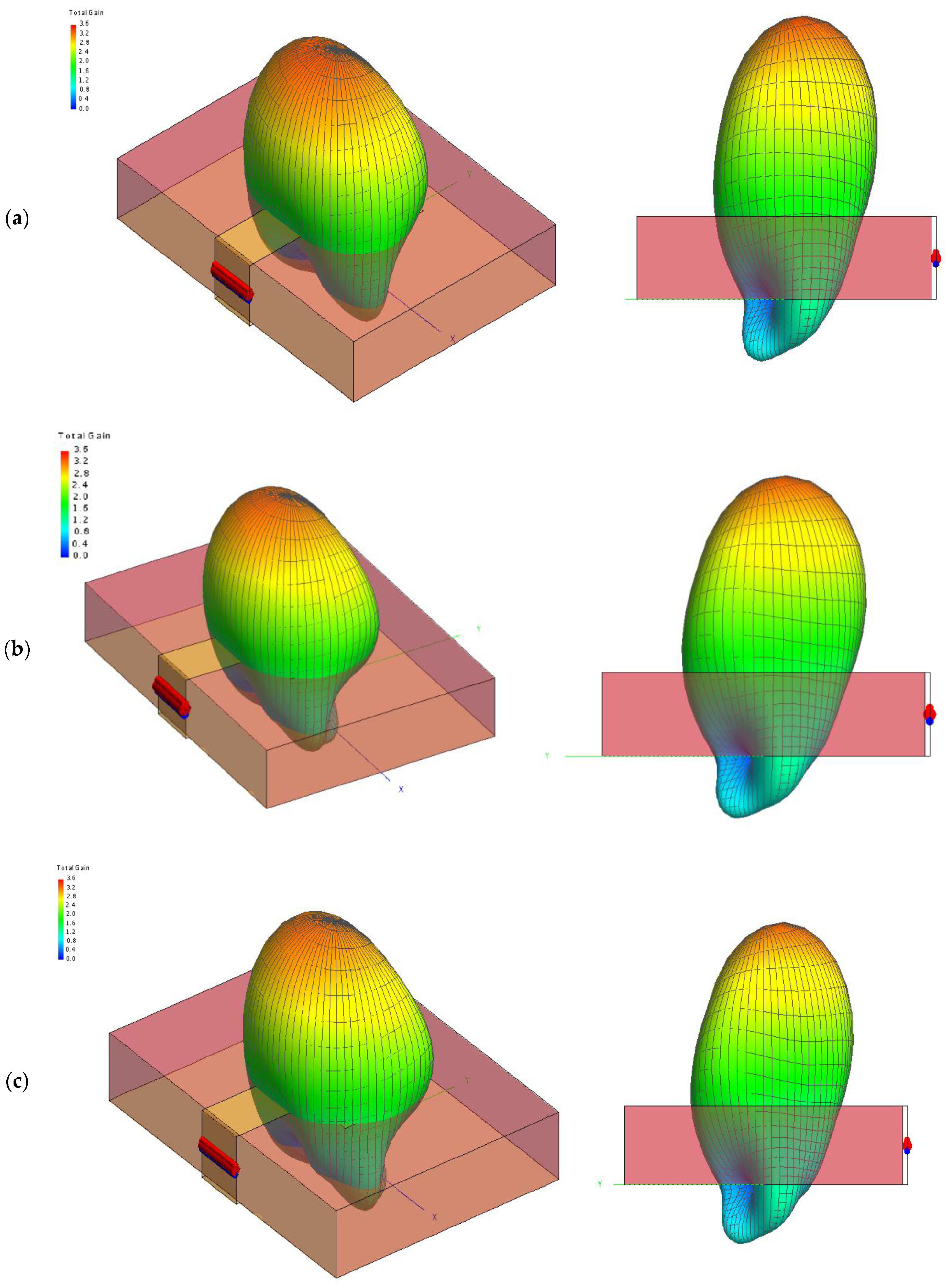
6.7. Radiation Characteristics

The radiation characteristics show how the antenna radiates energy depending on direction. It represents a standardized distribution of the electric field, or the relative distribution of surface power density. The characteristics are determined in two planes, i.e., horizontal and vertical, and can also be presented in a three-dimensional (3D) format [33,34]. The designed antenna should have directional radiation characteristics. A three-dimensional chart of the proposed antenna’s radiation characteristics for 27.51 GHz (a), 28.0 GHz (b), and 28.35 GHz (c) frequencies is shown in Figure 10. 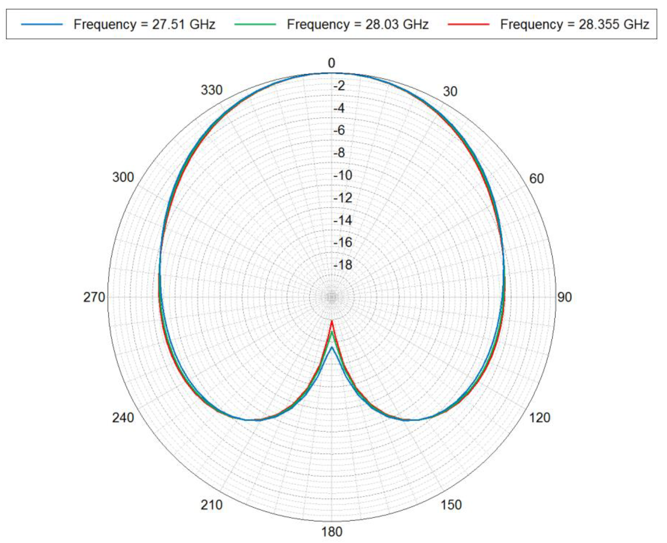Figure 11 shows the standardized radiation characteristics of the proposed antenna for 27.51 GHz (blue line), 28.0 GHz (green line), and 28.35 GHz (red line) frequencies in the polar coordinate system for vertical polarization. 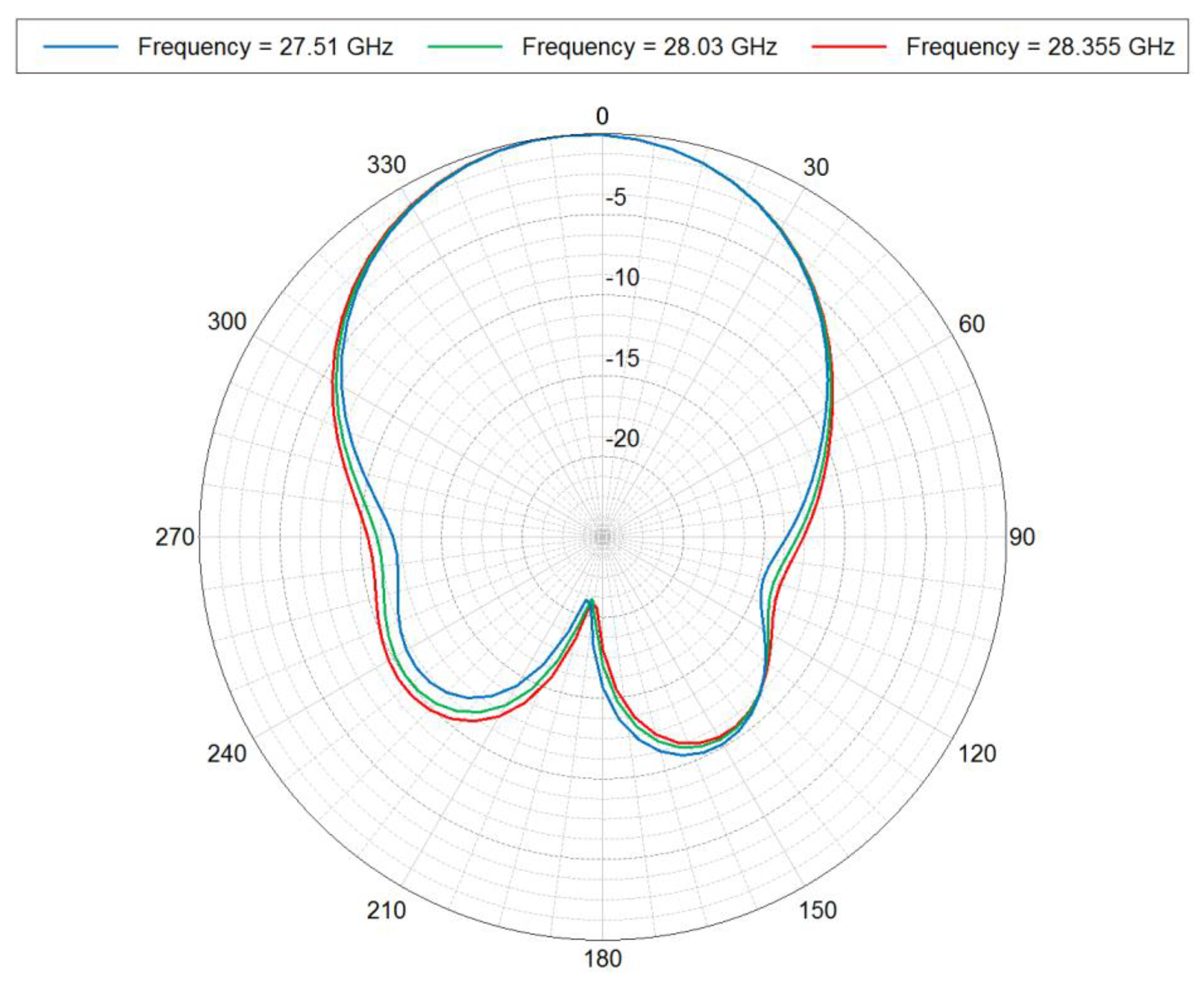Figure 12 shows the standardized radiation characteristics of the proposed antenna for 27.51 GHz (blue line), 28.0 GHz (green line), and 28.35 GHz (red line) frequencies in the polar coordinate system for horizontal polarization. The presented drawings show that the beam width at the –3 dB level for vertical polarization is 115.04° with the back lobe being −6 dB, while the beam width at the –3dB level for horizontal polarization is 72.16° with the back lobe being −10 dB.

7. Comparison of the Proposed Antenna with Other Antennas

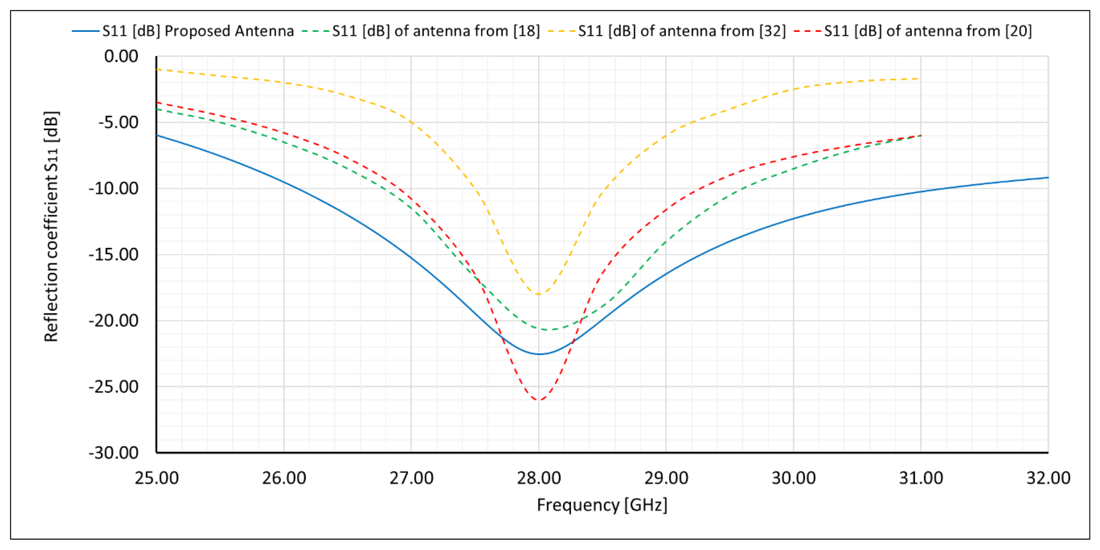
The obtained parameter values for the proposed microstrip antenna can be compared in terms of impedance matching and appropriate bandwidth, with other published results for the purposes of comparative evaluation. For example, the frequency response of the measured S₁₁ parameter of the proposed antenna may not be the lowest as compared with the S₁₁ values obtained for the antennas presented in [18,20,32], but it is relatively low.

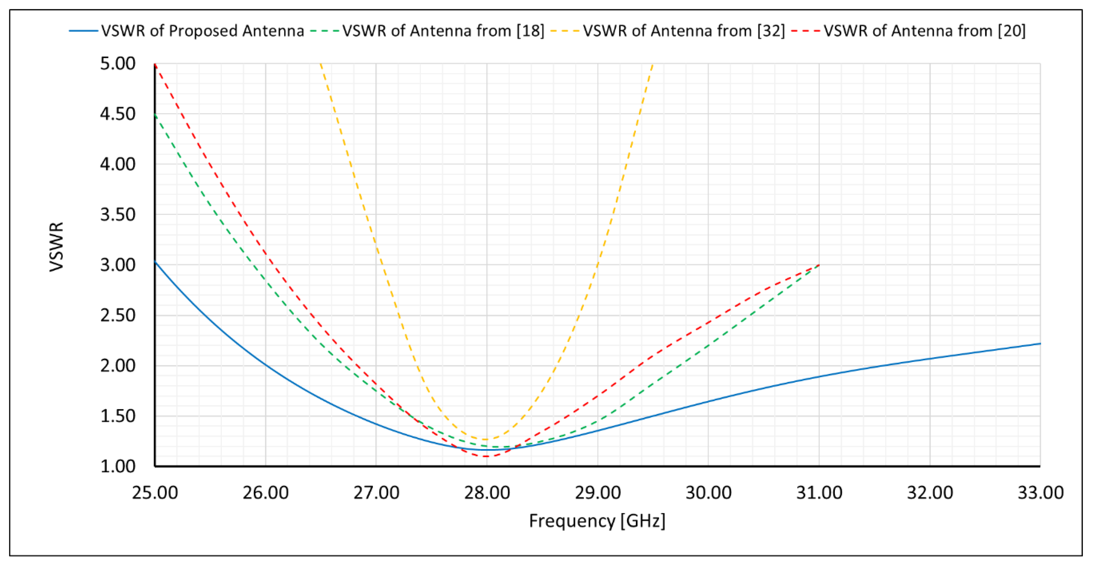
Figure 13 shows a comparison of the reflection factor as a function of frequency for the proposed antenna, and the antennas developed in other works. The corresponding frequency responses using the VSWR parameter are compared with each other, as shown in Figure 14.

The minimum reflection loss value obtained in this study is about −22.51 dB (VSWR ≈ 1.16), while in [20] it is about −26.00 dB (VSWR ≈ 1.10), in [18] it is about −21.00 dB (VSWR ≈ 1.20), and in [32] it is about −18.00 dB (VSWR ≈ 1.28). Moreover, for the antenna proposed in this work, the operating band of the antenna (BW) is the largest, amounting to S₁₁ ≤ −10 dB (VSWR ≤ 2) 5.57 GHz, and is centered exactly at 28 GHz, while in [20] the operating band is 2. 63 GHz and is also centered exactly at 28 GHz, in [18] the operating band is 2.85 GHz and is also centered at about 28.1 GHz (shift of about 100 MHz), and in [32] the operating band is 1.07 GHz and is also centered exactly at 28 GHz.

A comparative summary of the proposed antenna with the antennas described in [18,20,32] is presented in

Table 3. Comparisons among the bandwidth achieved in the present work to those achieved in other published works.

Performance Measure		Present Work (Proposed Antenna)	Work of [18]	Work of [20]	Work of [32]
Center frequency		28.00 GHz	28.10 GHz	28.00 GHz	28.00 GHz
BW	VSWR ≤ 1.25	1.15 GHz	0.45 GHz	0.79 GHz	NA
	VSWR ≤ 1.5	2.68 GHz	1.74 GHz	1.57 GHz	0.55 GHz
	VSWR ≤ 2	5.57 GHz	2.85 GHz	2.63 GHz	1.07 GHz
Relative BW		19.89%	10.14%	9.39%	3.83%
Gain		5.06 dBi	6.59 dBi	6.37 dBi	6.72 dBi

. It shows that the proposed microstrip antenna in this work has the best impedance matching bandwidth performance in all cases, especially for stringent matching conditions (VSWR ≤2, VSWR ≤1.5, and VSWR ≤1.25).

8. Conclusions

A rectangular microstrip antenna has been proposed for 5G applications in response to the growing demand for mobile data and mobile devices. This antenna has a resonance frequency of 28.00 GHz, for which the reflectance is equal to −22.50 dB. The proposed antenna has a radiation efficiency of 80.18% and the antenna gain for the resonance frequency is 5.06 dB. The results also show that its bandwidth is 5.57 GHz (relative operational band 19.89%), which is a very good result, much greater than results achieved in other published works, such as [15,16], where the operating bandwidth of the proposed antennas is around 1 or 2 GHz [18,19,20]. The proposed antenna would be a good option for 5G mobile communication, as it offers the high throughput required. The antenna is very compact and lightweight, which makes it suitable for devices where space is a major limitation.