1. Introduction
Air transport is considered to be the safest mode of mass transportation [
1]. ATM systems constitute one of the fundamental pillars that contribute to these high levels of safety. The essential function of ATM systems is to ensure that aircraft flying in the same airspace are kept separate from each other and from the ground.
The International Civil Aviation Organization (ICAO) defines ATM as “the dynamic, integrated management of air traffic and airspace including air traffic services, airspace management, and air traffic flow management—safely, economically, and efficiently—through the provision of facilities and seamless services in collaboration with all parties and involving airborne and ground-based functions”. Each country is responsible for ensuring that its airspace has an adequate ATM system.
The main objective of an ATM system is, therefore, to manage and reduce the risk of accidents. As such, the minimum separation distances between aircraft are defined as the minimum separation between two aircraft in the airspace to ensure that they do not collide with one other. The ATM is responsible for ensuring that these separation minima between aircraft are not violated and, in this way, managing the risk of collision between aircraft.
The safety of ATM systems has steadily improved over the last decades thanks to a number of measures including better equipment, technologies, and work procedures, as well as the deployment of additional safety barriers. However, the sustained growth of air transport imposes increasing demands and requirements on the safety, capacity, and efficiency of the ATM system.
ATM systems are currently facing their greatest challenge to date, namely the evolution towards multi-faceted, hyper-dimensional, highly distributed, and mutually dependent systems, with levels of complexity that were unimaginable just a few decades ago [
2]. The Single European Sky ATM Research (SESAR) project proposes a new paradigm for the ATM system of the future, primarily focused on technology and automation [
3,
4]. This system implies an architecture heavily influenced by digitalization and the geographic relocation of services.
It is increasingly challenging to maintain extremely high levels of safety in this complex and ever-changing environment. Ensuring that the level of safety provided by ATM systems is consistent with future needs and expectations, and that it is not negatively affected during the process of transition, is a priority for the aeronautical community.
Within the framework of the Single European Sky (SES), the European Union has several mechanisms to promote the cohesion, efficiency, and modernization of ATM systems. One of these mechanisms is the definition of a performance measurement framework that sets objectives in four key performance areas for European ATM systems, namely, safety, capacity, efficiency, and the environment. Safety is the most relevant of these areas, over and above the other three. As part of this monitoring and evaluation model, stakeholders must collect and study safety-related information to predict and anticipate not only current safety risks, but also emerging ones.
The main risk that an ATM must safeguard against is the occurrence of violations of the separation minima between aircraft, the so-called separation minima infringements (SMIs) [
5]. According to the European Aviation Safety Agency (EASA), the occurrence of SMIs is the second most important risk for European aviation [
6]. EUROCONTROL registered 827 and 930 incidents of severities A and B (high severity) during 2017 and 2018, respectively [
7]. Of these, 287 incidents in 2017 and 341 incidents in 2018 corresponded to non-compliance with separation minima between aircraft.
According to the Airborne Conflict Safety Forum, there are approximately 150 losses of separation for every million flights in European airspace [
8]. Considering that, on average, each flight receives 15 instructions from air traffic control en route, this means one loss of separation for every 100,000 instructions.
Although the number of SMIs is small compared to the volume of traffic, these are considered to be critical safety events due to the severity of their potential consequences. The monitoring of ATM-related safety events effectively boils down to monitoring the number of SMIs.
Furthermore, ATM systems constitute a highly regulated and standardized environment, which obeys a common standard set out by EASA. These regulations cover essential business processes and are common to all European countries. Based on these standards, the companies that manage ATM systems, air navigation service providers (ANSPs), have common technology, operating procedures, and work practices. They also apply similar business management principles, with comparable processes for setting goals, planning, and managing quality and safety. Their workers carry out the same functions, with equivalent levels of preparation and training regardless of the European country in which a company provides its services. In addition, they are subject to external audit processes to guarantee equivalent performance, efficiency, and safety in each country. As such, the aim is to ensure that the level of safety provided to all flights that cross European airspace is the same, regardless of the country overflown.
The high degree of homogenization between ANSPs should guarantee an equivalent underlying level of safety between different airspaces, so that the rate of occurrence of SMIs would be similar for all of them. However, despite the high level of standardization between ATM systems and ANSPs, they are affected by different local and specific circumstances that influence the service provided and, therefore, the quality and safety. The most significant of these factors are the volume of air traffic and its complexity [
9,
10].
In this regard, one of the main concerns of the industry is the underlying common level of safety, and the extent to which the different ATM systems and ANSP providers stick to or deviate from that common level of safety depending on their specific circumstances.
Given this situation, the monitoring and measurement of safety events, especially SMIs, must improve. Safety analysts and other decision makers within the aviation industry currently have to make safety assessments based on statistically incomplete information. Data on the number of losses of separation between aircraft is scarce and incomplete, partly due to their low occurrence and partly due to the sensitive nature of this information. Furthermore, the statistical models and techniques applied in the sector do not exploit the potential of the most advanced inference methods. It is of utmost importance that the most advanced techniques and methods are widely used to infer the rates of occurrence of safety events and to predict adverse safety effects.
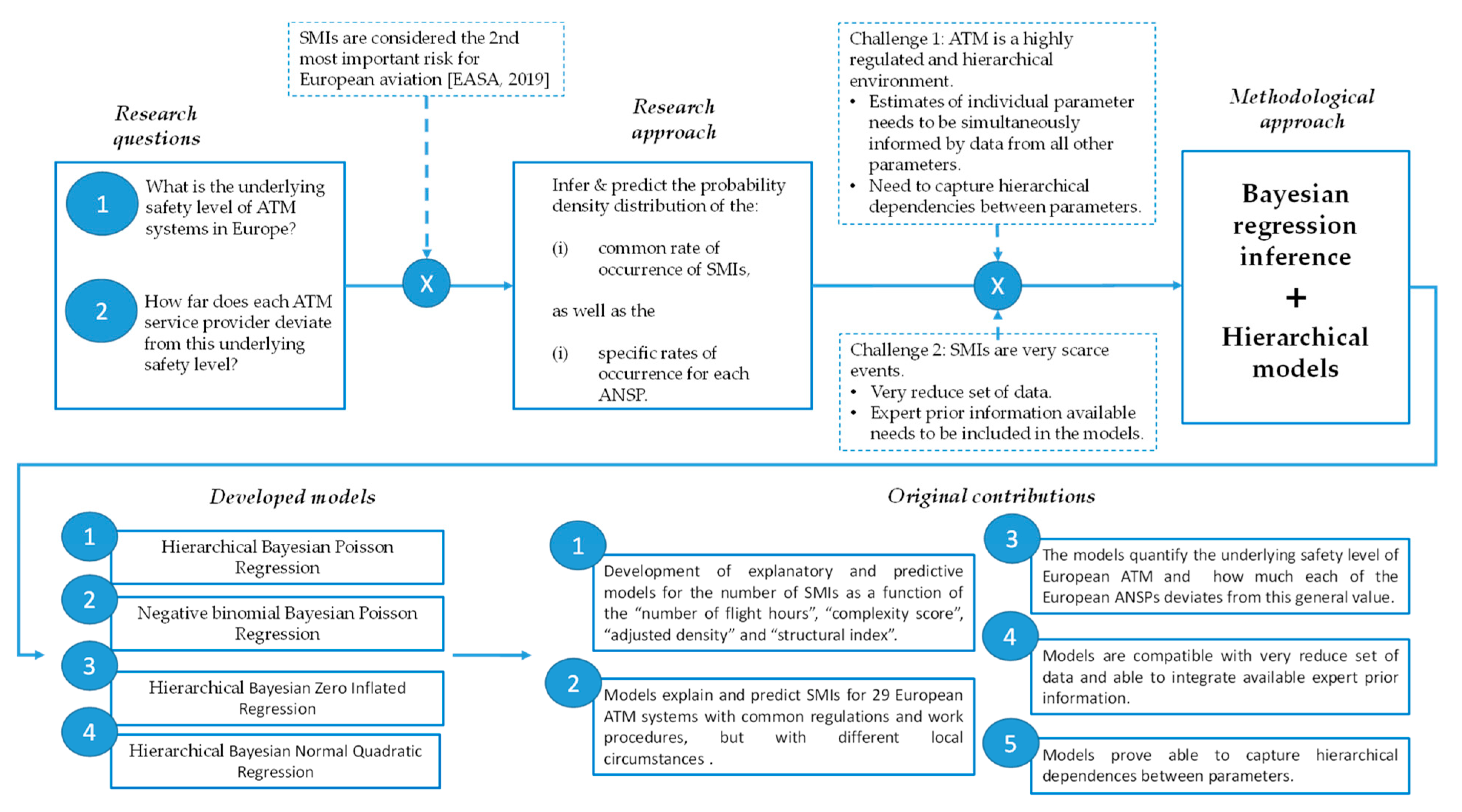
In this paper, we wish to answer two questions: (i) What is the underlying safety level in Europe? and (ii) What is the dispersion, that is, how far does each ATM service provider deviate from this underlying safety level? To do this, we will use hierarchical Bayesian inference models that allow us to infer and predict the common rate of occurrence of SMIs, as well as the specific rates of occurrence for each ANSP.
Studies and models regarding SMIs have focused, over the past few years, on technical aspects and human error as main causes of unsafe situations [
10,
11]. Some authors have partially analyzed some design aspects such as traffic mix [
5,
12,
13], relative geometry between aircraft [
14], complexity of airspace sectors [
4], air traffic controller workload, or flight efficiency. However, none of these approaches incorporate predictive capabilities, nor allow benchmarking between ANSP.
Additionally, given the high level of safety in the industry, SMIs respond at very low frequencies of occurrence, and it is very difficult have a sufficient number of data for relevant conventional statistical analysis [
15,
16,
17].
Hierarchical and Bayesian models have been used in recent decades to overcome these limitations and to predict safety incidents in other modes of transport, specifically in road transport [
18]. However, within the aviation context, there is yet little research in this area [
19].
Bayesian models are useful for performing this type of analysis, because they permit inference of the statistical parameters and the distributions being studied in spite of the fact that little data is available [
20,
21]. They allow a priori knowledge about the phenomenon under study to be incorporated [
22,
23,
24]. They also permit various levels or hierarchies to be considered when explaining the different phenomena. Furthermore, they allow information from different sources to be integrated in an orderly manner [
22]. As such, in this article, we propose and evaluate several Bayesian models that consider the hierarchical relationship between the ANSPs and illustrate the underlying mechanism in the generation of SMIs from explanatory variables that represent the main local differences.
These models are intended to explain and predict the safety performance of 29 European organizations, with common regulations and work procedures, but with different circumstances and numbers of aircraft, each managing traffic of differing complexity.
Figure 1 outlines the process and highlights the original contributions of the paper.
2. Hierarchical Bayesian Models
Hierarchical models are mathematical representations that involve multiple parameters in such a way that credible values of some of the parameters depend significantly on the values of other parameters. Hierarchical Bayesian models have been used in different industries to analyze different aspects of safety [
18,
20,
23,
24,
25] but have not yet been regularly used in aviation [
11,
21,
22,
26,
27].
What makes hierarchical modelling so effective is that the estimate of each individual parameter is simultaneously informed by data from all other parameters. All parameters inform the top-level parameters, which in turn restrict all individual parameters. These structural dependencies provide better-informed, that is, more precise estimates of all parameters.
Consider that each ATM system will experience a certain number of SMIs per year. Each ATM will provide service to a certain number of aircraft in its airspace. Parameter defines the rate of occurrence of SMIs for each ATM system. can be estimated from the number of SMIs that have occurred in the past, the number of flights managed, and their complexity. Similarly, given that all ATM systems operate according to the same rules and procedures, each parameter will depend on a global parameter that defines the rate of occurrence of SMIs of a generic ATM system that applies the rules and procedures deriving from the European regulations. This hierarchy of dependencies between parameters could be extended to even more levels, bearing in mind that, over and above European regulations, ATM systems around the world are governed by ICAO standards.
In hierarchical models, parameters at different levels co-exist in a joint parameter space. The joint prior distribution can be factored or decomposed so that some parameters depend on others. In other words, chains of dependencies can be established between parameters. These factorizations are not unique, and each model can choose the most convenient parameterization at any time.
Given a series of parameters
and
ω, and a set of data
D, we can apply Bayes’ theorem as follows:
What characterizes a hierarchical model is that the terms on the right side of Equation (1) can be factored into a chain of dependencies, as seen in Equation (2):
According to this refactoring, the data, D, depends only on each parameter . This means that once the value of the parameter has been established, the data becomes independent of all other parameters. It is also clear that the value of each parameter depends on the value of ω, and its value is conditionally independent of all other parameters. In other words, when the value of ω is set, becomes independent of all other parameters. Any model that can be factored or decomposed into a chain of dependencies like that given in Equation (2) is a hierarchical model.
Hierarchical dependencies between parameters enable all available data to be used to jointly inform the estimated values of the parameters. In our case, this means that data from each ATM system can be used to estimate the parameters of the other ATM service providers. In turn, the data from all providers can be used together to estimate the ω parameter, which gives the rate of occurrence of SMIs of a generic ATM system.
3. Data Used
The data used in this study were obtained from a number of European institutions involved in monitoring the performance of ATM systems, including the Performance Review Body (PRB), the Performance Review Unit (PRU), and EASA.
The PRB is an advisory body of the European Commission that assists the Commission and national authorities in the supervision of the performance of ATM systems. The PRU is part of the EUROCONTROL Single Sky Directorate. It provides information and data analysis on the performance of European ATM. EASA collaborates with the two aforementioned institutions by collecting the necessary safety data in each state.
The study covers a total of 29 European states. The value to be estimated and predicted is the number of annual SMIs that have taken place in each of the 29 ATM systems included in the study. The variable is to the number of annual SMIs. Subscript relates to the year, and subscript relates to the specific ATM system.
Specialist literature on the topic suggests that the two factors that best explain the occurrence of SMIs are the volume of air traffic and the complexity of this traffic. To verify these dependencies, the following explanatory variables are analyzed in the study.
is the volume of air traffic, i.e., number of annual flight hours, defined as the number of total flight hours per year of aircraft operating under Instruments Flight Rules (IFR) in the airspace of each of the countries considered in the study. The subscripts and refer to the year and ATM system, respectively.
To assess the complexity of air traffic, Eurocontrol has defined a set of indicators that can be used for ANSP benchmarking [
28]. The complexity indicators are based on the “interactions” that arise when there are two aircraft in the same “place” at the same “time”. The variable “complexity score”
is defined as the total duration in minutes per flight hour of all interactions between controlled aircraft in a given volume of airspace.
The indicator “complexity score” is the product of two components: the adjusted density and the structural index . The variable measures the relative concentration of aircraft in the airspace. The airspace is divided into a discrete grid of cells measuring 20 × 20 nautical miles in the horizontal and 3000 feet high. An interaction is defined as the simultaneous presence of two planes in one of these cells. The variable is the sum of horizontal, vertical, and velocity interactions.
In this study, the values for complexity score, adjusted density, and structural index are aggregated on an annual basis. Therefore, the variables refer to the annual mean value (calculated as the sum of the daily values of a year divided by the total flight hours in the year). The subscript indicates the year in question, and the subscript indicates the ATM system analyzed.
The above data was obtained for 29 countries and their ATM systems over seven consecutive years. The identity of the countries is not given in the study. Each has been assigned a number from 1 to 29. In total, the data sample comprises five variables with 203 records per variable.
Figure 2 shows the relationship between variables
by means of scatterplots and the calculation of the correlations between them, as well as the density functions of each variable. The value of the variable
“number of flight hours” is divided by 100,000 so that it is more easily readable in the figure.
Figure 3 shows a boxplot for the number of SMIs per year.
Figure 4 gives a boxplot of the number of SMIs for each ANSP.
Figure 5 shows the evolution of the number of SMIs versus the number of flight hours. Each ANSP is identified by a unique color.
4. Proposed Hierarchical Models
The models analyzed in this study combine regression analysis with hierarchical structures [
29,
30].
Let
be the predicted variable and let
be the predictors. There is a likelihood function that expresses the probability of the values of the predicted variable as a function of the values of the predictors. Generalized Linear Models (GLM) are used that express the combined influence of the predictors as their weighted sum. Function
of the predictors is defined as:
where
refers to each measurement and
relates to each ATM system.
Each coefficient represents the expected variation in the predicted variable due to a unit increase in the value of the predictor .
Likewise, prior distributions are defined for the coefficients
:
depends in turn on other hyperparameters that enable the relationship between the different ATM systems and the general safety standard to be expressed via a hierarchical relationship. is defined as a Beta distribution of parameters , .
According to [
31], analysis of the first and second moments of a distribution
can be reparametrised as follows:
Parameter represents the mean or overall influence of the variable on the precicted variable, while parameter is a measure of the dispersion around parameter . Parameter is inversely proportional to the variance (), as such, it is an appropriate indicator of the dispersión of characteristic of each ATM system. The higher the value of the paramater for an ATM system, the lower the variance, and, therefore, the influence of the variable on the number of SMIs will be closer to the overall mean value for Europe. Conversely, the lower the value of the parameter , the greater the dispersión.
Taking this reparameterization into account, the prior distributions of the coefficients
are:
Once the predictors are combined, they are mapped with the predicted variable. Firstly, an inverse link function
must be defined according to the following equation:
where
represents the central tendency of the prediction of the values of
.
This central tendency
may correspond to the mean or any applicable measure of central tendency, such as mode, median, etc. The only thing that remains to do is to specify the probability density function, abbreviated as
, which enables the measurements
to be generated from the central tendency
. The literature generally refers to this probability distribution as the noise distribution.
The shape of the probability density function will depend on the scale of measurement of the predicted variable. In our problem, all the predictive variables correspond to metric data, while the predicted variable corresponds to count data, a particular case of metric data.
If the predicted variable corresponds to count data, the typical
distribution is usually a Poisson distribution. The canonical link function for Poisson distribution is a log–link function [
32]. The combination of both results in a Poisson regression, as indicated below:
As can be seen, a Poisson regression is a type of generalized linear model (GLM) that enables a non-negative integer response, that is, a natural number, to be modelled against a linear predictor via an exponential link function. The exponential link function allows us to transform the expected values of the response found on the scale of (0, ∞) into the scale of the linear predictor, that is (−∞, ∞).
To mitigate the limitations due to overdispersion in the data, three additional models have been tested.
Hierarchical negative binomial regression model. The negative binomial model is parameterized in terms of the mean (
) and the scale factor (
[
33]. It can be likened to a hierarchical two-stage process in which the response is modelled against a Poisson distribution whose expected recount is in turn modelled by a Gamma distribution with a mean
and a constant scale parameter (
).
where the expected value of
is given by
and the variance is
.
The negative binomial model is appropriate for situations of over-dispersion caused by clustering (due to the influence of other factors that have not been measured). JAGS is Just Another Gibbs Sampler, a program for analysis of Bayesian hierarchical models using MCMC) that uses a parametrization of the negative binomial distribution based on the parameters
and
. Direct estimation of the parameters
and
of the binomial distribution usually implies a bad autocorrelation of the MCMC chains. To avoid this problem, we will use a reparameterization in which we will set priors for the mean
and the parameter
, while the variance and the parameter p will be obtained from
and the parameter
.
Hierarchical zero-inflated regression model regression. This model is appropriate when the overdispersion is due to a higher-than-expected number of zeros in a Poisson distribution [
34]. Zero-inflated models combine a binary logistic regression model with a Poisson regression.
Hierarchical normal quadratic regression with variance proportional to the number of flights. This last model combines the advantages of Poisson distributions with a normal model [
35,
36]. This allows a variance proportional to the number of SMIs to be combined with the effect of stable confidence intervals, especially if the number of incidents is high, which gives rise to a quadratic regression.
The data points are assumed to derive from a normal distribution. The model establishes a different variance for each ATM system proportional to the number of flights handled by each organization. A Gaussian noise is added to the regression to account for cases where the variance is constant. The hierarchical structure of parameters is similar to that of the previous models.
Table 1 summarizes the mathematical formulation of the models developed.
5. Evaluation of the Models
All the models in this study have been developed using MCMC [
37] simulations based on Gibbs using the JAGS simulation program [
38]. The most significant results of each model are summarized below.
5.1. Model 1
Figure 6 and
Figure 7 give the overall result and precision of Model 1.
Figure 6 shows the values predicted by Model 1 (in red) and the real values (in black). It also gives the confidence intervals at 2.5% and 97.5%, respectively (red lines), and the mean value of the prediction (black line). It is clear from
Figure 4 that the 95% interval does not contain all of the SMIs and that the prediction is less optimal for high values of flight hours.
Figure 7 shows the residuals of the model, the predicted values versus residuals, and the Q–Q plot. The residual plot shows a high density of points close to the origin and a low density of points away from the origin. It is symmetric about the origin, and there are not any patterns in the value of the residuals as we move along the
x-axis. A small number of cases have notable errors. There are nine measurements with errors greater than 50. These correspond to ANSPs 9, 11, 22, 28, 8, 20, and 12.
Figure 8 comprises caterpillar plots giving the distributions of each hyperparameter
of the model (K, K1, K2, K3, and K4). Each distribution is indicated by a horizontal line representing the 95% interval and a dot showing the mean value. Each provider is non-dimensionalized by assigning a number to it. The vertical red line represents the global mean of the means of the posterior distributions. Each
parameter is a measure of the dispersion of the regression model coefficients for each service provider. The higher the value of
, the lower the variance and, therefore, the nearer the value of the parameter for an ANSP to the mean value of the
parameters at a European level. Conversely, the smaller the value of
, the greater the dispersion. It should be borne in mind that all values of
are common for all ANSPs.
The numbers show that the mean values of are generally high. This is in agreement with the hypothesis that the coefficients of the regression model are of the same order for the ANSPs and similar to the corresponding value. However, in each case, there is a set of service providers whose behavior deviates significantly from the mean. Extreme values of , that is, values that are unusually high or low compared to the mean values, can be helpful in identifying ANSPs with atypical rates of incidents.
For different ANSPs, the parameters that show the most variation are K1, K2, and K3. In other words, the variability in response between ANSPs is greater for the variables x1 “number of flight hours”, x2 “Complexity Score”, and x3 “Adjusted Density”, in that order.
Finally, the values of
for this model are summarized in
Table 2.
5.2. Model 2
Figure 9 and
Figure 10 give the overall results and the precision of Model 2. In this model, the 95% interval contains all of the SMIs, but at the expense of very wide confidence intervals, which grow exponentially with increasing number of flight hours. It is also at the expense of poor precision for high values of number of flight hours, as can be seen in the right-hand margin of
Figure 9.
The precision and fit of this model are worse than the previous one. Some values shown in
Figure 8 have very high residuals (greater than 600). The plot of residuals versus predicted values shows an increase in error and spread as the predicted values increase. This same effect can be seen at the edges of the Q–Q plot. These effects are especially due to the inability of the model to reproduce the seven data points at the far right of the diagram. This data corresponds entirely to a single ANSP, number 9. For the remaining data and ANSPs the model fits well. Furthermore, there are eight measurements with errors greater than 50, which correspond to ANSPs 9, 22, 28, 20, and 12.
Figure 11 comprises caterpillar plots giving the distributions of each hyperparameter
of the model. The numbers show that the mean values of
are generally high. The graphs show that in the case of parameters K and K4 there is no dispersion, and that for parameters K1, K2, and K3, dispersion is limited to a few service providers, notably ANSPs 13, 8, 22, 19, 6, 10, and 29. This coincides with the analysis of
Figure 10.
Finally, the values of
for this model are summarized in
Table 2.
5.3. Model 3
Figure 12 and
Figure 13 show the overall result and precision of Model 3. Model 3 behaves in a similar way to Model 1. It must be remembered that the zero-inflated model has been designed as a variation of the Poisson model, with a component that introduces a binomial model to account for an excess of zeros. However, the estimate of parameter
(see
Table 3) with a mean value of 980 and a similar standard deviation, namely 997, indicates that the binomial model does not give a good fit.
This model contributes very little in addition to Model 1. This is because the difficulty in achieving a good fit is not caused by an excess of zeros but rather due to difficulties in reproducing the high-number SMIs.
Table 3 shows that the values of the hyperparameters
are similar to those obtained using Model 1. Similarly, in this model there are eight measurements with errors greater than 50, which correspond to the ANSPs 9, 22, 28, 20, and 12.
Figure 14 comprises caterpillar plots giving the distributions of each hyperparameter
of the model (K, K1, K2, K3, and K4).
5.4. Model 4
Figure 15 and
Figure 16 give the overall result and the precision of Model 4. The main advantage of this model, compared to the previous ones, is that the confidence levels give a very good fit to the data and the predictions are, in all cases, in line with the initial data.
This model has more parameters than the previous ones. In particular, the introduction of the error parameter permits fine-tuning of the data of each ANSP. This means that it is flexible and capable of quantifying the dispersion of the data.
In this model, the hyperparameters
K, K1, K2, K3, and K4) and
,
,
) behave in a similar manner to the way they do in the other models.
Figure 17 gives an analysis of the caterpillar plots of the
parameters of the regression function. This enables us to have a more intuitive view of the influence of the variables
on each ANSP.
Additionally, in this model, there is another consideration with respect to the parameter in that it corresponds to the coefficient of the quadratic term in the regression. This parameter can be used to reflect the dependence of the rate of occurrence of SMIs on the number of flight hours. In aviation this phenomenon is known as the stress effect and refers to the increase in accident rates as a function of the number of operations or flight hours. This has not been considered in the other three models. The value of the quadratic coefficient in the regression parameter is a measure of the importance of the stress effect. The higher the value of , the greater the positive correlation between the rate of occurrence of SMIs and the square of the number of flight hours and, consequently, the greater the stress effect. ANSPs that experience this effect are considered to be saturated, since variations in the number of flight hours have a significant effect on the occurrence of SMIs. Therefore, special attention must be paid to this factor.
Analysis of the parameters
, the error term in the linear regression, and
the variance proportional to the number of hours of operation, is especially relevant in this case.
Figure 18 shows the caterpillar plots for these variables.
Practically all the ANSPs have values of equal to zero with the exception of ANSPs 29, 18, 19, 21, 25, 7, and 6. All of these correspond to small service providers with low numbers of flight hours.
Finally, the values of
,
,
) for all the models are summarized in
Table 2.
6. Comparison of the Models
The four hierarchical models in the study use the following probability density functions: Poisson, negative binomial, zero-inflated, and normal. We will use deviation information criteria (DIC) to compare the models [
39] via MCMC simulations.
This parameter calculates the deviation as the mean of the posterior predictive function:
This criterion is a measure of the goodness of fit of the data and, at the same time, introduces a term to evaluate the complexity of the model. This criterion is asymptotically the same as performing cross-validation using part of the data to estimate the data and the rest to calculate the goodness of the predictions [
40]. The lower the calculated DIC value, the more accurate the model’s predictions. One model can be considered superior to another when its DIC is more than five points below that of its competitor [
41].
According to the values obtained in the simulation, Model 4 appears to be the most efficient and Model 2 the least efficient. This coincides with the analysis carried out in the previous sections. The table confirms that Models 1 and 4 are better at predicting SMIs. For small values of SMIs, the Poisson model (Model 1) is more efficient, while for high values of SMIs, the normal model (Model 4) is more accurate. For intermediate values, all models behave in a similar manner. The DIC values for Models 1 and 3 are similar.
The hierarchical relationship framework underlying all the models includes parameters and . Each of the models includes a parameter or set of parameters that synthesizes the general level of safety of the EU ATM system. Parameter represents the mean or overall influence of variable on the predicted variable. Parameter is a measure of the dispersion of an ANSP around parameter . These parameters could be used in further studies to benchmark among different regions in the world (USA, Middle East, etc.), providing similar data set are available for all the regions.
If the values of are high and similar to each other for all ANSPs, this means that there is a central tendency around the European mean, since is inversely proportional to the variance of . Conversely, small values of indicate that an ANSP has an unusually low or high number of SMIs, compared to the European average.
A value of that is significantly different to that of other ANSPs will alert us to those ANSPs whose behavior deviates from the ideal.
To illustrate the meaning of
let us analyze in detail an example. Let us look at parameter K4 in Model 1 (
Figure 8d). The estimated values of K4 for each of the 29 ANSPs are presented in
Table 4. K4 is related to the influence of the variable
, “complexity index”, in the number of SMIs. K4 indicates the deviation of each ANSP with respect to the influence of complexity index in the number of SMIs from the overall European ATM system. It can be observed that the values of K4 are higher than 900 for almost all ANSPs, except for ANSP-12 and ANSP-9.
is inversely proportional to the variance of
For those ANSPs with elevated K4 values, the influence of complexity index in the occurrence of SMIs is similar and close to that of the overall European ATM system. However, ANSPs 12 and 9 exhibit lower values of K4, 78 and 335, respectively, indicating that for these two providers the dependency of the SMIs with the variable complexity index does not behave as the overall EU ATM system.
In general, ANSPs exhibiting higher errors in each model happen to have low values for one or more parameters, which indicates higher deviation of this ANSP with respect to the influence of one explanatory variable in the number of SMIs, regarding the overall European ATM system.
Furthermore, the final model has two additional features. Firstly, it combines the advantages of Poisson distributions with a normal model. To do this, it introduces a variance proportional to the number of SMIs. When the variance of an ANSP is constant for the entire range of SMIs, the Gaussian noise added to the regression, allowing to be set to 0, if necessary. This model also has a quadratic term in the regression equation, which reflects the dependence of the rate of occurrence of SMIs on the square of the number of flight hours. In aviation, this phenomenon is known as the stress effect, and refers to the increase in accident rates as a function of number of flight hours.
7. Conclusions
This study makes use of the advantages of hierarchical Bayesian inference models to quantify the levels of safety in European airspace. The study has three objectives:
Generate predictive models that enable the number of losses of separation between aircraft in the airspace to be predicted using predictive variables such as the number of flight hours or the complexity of the airspace.
Estimate the general underlying safety level of European ATM systems.
Estimate how much each of the European ANSPs deviates from this general value.
For this, four models were developed that combine a hierarchical approach with a regression model. These enable us to infer and predict the common rate of occurrence of SMIs, as well as the specific rates of occurrence for each ANSP. The models take two factors into consideration: the hierarchical relationship between the ANSPs and the generation of SMIs from predictors that represent the main local differences.
The four models generally demonstrate good behavior. Model 4 is the most efficient and Model 2 the least efficient. For small values of SMIs, the Poisson model (Model 1) is more efficient, while for high values of SMIs the normal model (Model 4) is more accurate. For intermediate values, all models behave in a similar manner. The DIC values for Models 1 and 3 are similar.
The original pieces of knowledge provided by this research can be summarized as:
The development of explanatory and predictive models for the number of SMIs as a function of the “number of flight hours”, “complexity score”, “adjusted density”, and “structural index”.
The models quantify the underlying safety level of European ATM and how much each of the European ANSPs deviates from this general value.
The contribution of the European ATM regulation to a reduced number of SMIs has been quantified as an overall EU ATM system performance.
The models explain and predict SMIs for 29 European ATM systems with common regulations and work procedures, but with different local circumstances.
The models are compatible with a very reduced set of data and able to integrate available expert prior information.
The models prove to be able to capture hierarchical dependences between parameters.
The models developed have been found to be useful in explaining and predicting the safety performance of 29 European ATM systems with common regulations and work procedures, but with different circumstances and numbers of aircraft, each managing traffic of differing complexity.
This study shows the usefulness of hierarchical structures when it comes to obtaining parameters that enable risk to be quantified effectively. We can identify the parameters that are characteristic of the safe operation of each ATM system and of the entire European system. These parameters allow us to identify and quantify trends and establish benchmarks to compare the current year’s performance with that of previous years.


