An Entropy-Like Estimator for Robust Parameter Identification

Abstract

This paper describes the basic ideas behind a novel prediction error parameter identification algorithm exhibiting high robustness with respect to outlying data. Given the low sensitivity to outliers, these can be more easily identified by analysing the residuals of the fit. The devised cost function is inspired by the definition of entropy, although the method in itself does not exploit the stochastic meaning of entropy in its usual sense. After describing the most common alternative approaches for robust identification, the novel method is presented together with numerical examples for validation.

1. Introduction

In spite of their practical importance in many fields of science and technology, apparently there is no universal and well-accepted definition of outlying data. This may have resulted from the wide range of fields (statistics, data mining, signal processing, time-series analysis, system identification, telecommunications, etc.) dealing with outliers from different perspectives. Broadly speaking, we can think of outliers as data values that appear to be inconsistent with the rest of the set. In model identification for automatic control applications as well as in the other fields of science and technology, outlying data may have a dramatic impact on parameter estimation. This paper describes the basic ideas behind a novel prediction error parameter identification algorithm for static models exhibiting high robustness with respect to outlying data. Given the low sensitivity to outliers, these can be more easily identified by analysing the residuals of the fit. The proposed algorithm is based on the minimization of a particular cost function of the model prediction error residuals. The devised cost function is inspired by the definition of Gibbs’ entropy and shares the same mathematical properties of the entropy associated to a set of probability values $p_i$, although the method in itself does not exploit the stochastic or information theoretic meaning of entropy in its usual sense (hence the name entropy-like). Contrary to alternative robust parameter identification methods (as the Least Median of Squares (LMS)), if the model is sufficiently regular with respect to the parameter vector $\mathit{\theta }$, the derivatives of the proposed penalty function with respect to $\mathit{\theta }$ can be analytically computed allowing to exploit gradient and Hessian matrix information in the numerical minimization routine. Robustness to outliers is obtained as a consequence of the fact that the used cost function rewards unevenly distributed residuals rather than some kind of weighted mean square error (MSE). In particular, the minimization of the devised entropy-like function rewards the presence of a majority of low relative errors and a minority of large ones.

After reporting on the state of the art on robust parameter identification in Section 2., the proposed method is outlined and discussed in Section 3. The basic algorithm properties and associated problems are addressed in Section 4. and numerical results are provided in Section 5. Conclusions and future research directions are finally addressed in Section 6.

2. Robust Parameter Identification: A Brief Summary of the State of the Art

Consider a static system

$$y_i=f(x_{i1},x_{i2},\dots ,x_{im},{\mathit{\theta }}_r)+{\epsilon }_i:i=1,2,\dots ,N$$

(1)

being ${\mathit{\theta }}_r\in {\mathbb{R}}^{m\times 1}$ the unknown parameter vector, $y_i\in \mathbb{R}$ the response variable, $x_{i1},x_{i2},\dots ,x_{im}$ the explanatory variables and ${\epsilon }_i$ the error term. Index i runs on the number of observations N that is assumed to be strictly larger than m. The error term ${\epsilon }_i$ is assumed to be a normally distributed random variable with zero mean. Denoting with $Z_N=\{(y_i,x_{i1},x_{i2},\dots ,x_{im}):i=1,2,\dots ,N\}$ the set of the available observations, a regression estimator T is an algorithm associating to $Z_N$ an estimate $\widehat{\mathit{\theta }}$ of ${\mathit{\theta }}_r$, namely $T\left(Z_N\right)=\widehat{\mathit{\theta }}$. Prediction error estimators T are designed based on the properties of the regression residuals

$$r_i:=y_i-{\widehat{y}}_i$$

(2)

where ${\widehat{y}}_i$ are the predicted responses ${\widehat{y}}_i=f(x_{i1},x_{i2},\dots ,x_{im},\widehat{\mathit{\theta }})$. The most popular prediction error estimators are the Least Squares (LS) and weighted LS estimators defined respectively as

$$\begin{array}{ccc}\hfill {\widehat{\mathit{\theta }}}_{LS}& =& arg\underset{\mathit{\theta }}{min}\sum _{i=1}^N{r}_i^2=arg\underset{\mathit{\theta }}{min}\left({\mathbf{r}}^T\mathbf{r}\right)\hfill \end{array}$$

(3)

$$\begin{array}{ccc}\hfill {\widehat{\mathit{\theta }}}_{WLS}& =& arg\underset{\mathit{\theta }}{min}\left({\mathbf{r}}^T\Gamma \mathbf{r}\right)\hfill \end{array}$$

(4)

where $\mathbf{r}\in {\mathbb{R}}^{N\times 1}$ is the residual vector $\mathbf{r}={(r_1,r_2,\dots ,r_N)}^T$ and $\Gamma \in {\mathbb{R}}^{N\times N}$ a symmetric positive definite (or eventually semidefinite) matrix of weights. Given the symmetric nature of Γ, there is no substantial loss of generality in assuming it to be diagonal, i.e., there exists an orthogonal $N\times N$ matrix Ω such that $\Omega \Gamma {\Omega }^T=$ diag$({\gamma }_1,{\gamma }_2,\dots ,{\gamma }_N)$, so that the WLS estimator results in

$${\widehat{\mathit{\theta }}}_{WLS}=arg\underset{\mathit{\theta }}{min}\sum _{i=1}^N{\gamma }_i{\tilde{r}}_i^2$$

(5)

where $\tilde{\mathbf{r}}=\Omega \mathbf{r}$. If the weight matrix Γ in the WLS estimator is chosen to be the covariance of the zero mean normally distributed error term $\mathit{\epsilon }={({\epsilon }_1,{\epsilon }_2,\dots ,{\epsilon }_N)}^T$, namely $\Gamma =E\left[\mathit{\epsilon }{\mathit{\epsilon }}^T\right]$, the corresponding estimator (some times called the Markov Estimator) coincides with the Maximum Likelihood (ML) estimator defined as

$${\widehat{\mathit{\theta }}}_{ML}=arg\underset{\mathit{\theta }}{max}p\left(Z_N\left|\mathit{\theta }\right.\right)$$

(6)

where $p\left(Z_N\left|\mathit{\theta }\right.\right)$ is the probability of the data set $Z_N$ given $\mathit{\theta }$.

If, moreover, the error terms ${\epsilon }_i$ are assumed to be independent and identically distributed (i.i.d.) the above ML estimator minimizes the sample version of the entropy associated to $p(·)$, namely

$${\widehat{\mathit{\theta }}}_{ML}=arg\underset{\mathit{\theta }}{min}\sum _{i=1}^N-logp\left({\epsilon }_i\left|\mathit{\theta }\right.\right).$$

(7)

The properties of the celebrated Maximum Likelihood, Least Squares and Weighted Least Squares estimators are very well known and will not be discussed here. Yet it should be stressed that these methods are also very well known to be highly sensitive to outliers [1, 2], i.e., to elements of $Z_N$ that do not comply with the model (1). Intuitively the lack of robustness of all ML related methods should not surprise: if $Z_N$ is contaminated by wrong data (i.e., data that should not be in $Z_N$), maximizing the likelihood of $Z_N$ conditioned to $\mathit{\theta }$ means maximizing the probability that the data set does contain wrong data.

The issue of designing robust (with respect to outliers) parameter estimators has been explored in many fields of science following often different approaches. In order to motivate and compare the solution proposed in this paper with the state of the art, some of the alternative known approaches are briefly summarized: based on the observation that the ML estimator minimizes the sample version of the entropy associated to the i.i.d. model errors ${\epsilon }_i$, in [3, 4] a minimum entropy (ME) estimator is proposed. The main idea consists in estimating the probability density function of residuals $\widehat{p}\left(r_i\left(\mathit{\theta }\right)\right)$ with a kernel based method (using radial basis functions, by example) and then computing the parameter vector estimate ${\widehat{\mathit{\theta }}}_{ME}$ as the argument minimizing the entropy associated to $\widehat{p}$. The idea behind this approach is that minimizing the estimated entropy of the residuals will force them to have a minimum dispersion. This approach, although computationally demanding, is indeed appealing and has also been pursued within system identification in [5].

A different perspective to the problem can be found in the rich statistics literature on the subject. A milestone reference is the book by Peter J. Huber [2] describing (among the rest) the use of M-estimators (where the M is reminiscent of Maximum Likelihood). M-estimators can be thought of as generalizations of the LS estimator (3) where the square of residuals is replaced by an alternative penalty function $\rho (·)$ with a unique zero in the origin and such that $\rho \left(z\right)=\rho (-z)$, namely

$${\widehat{\mathit{\theta }}}_M=arg\underset{\mathit{\theta }}{min}\sum _{i=1}^N\rho \left(r_i\left(\mathit{\theta }\right)\right).$$

(8)

Indeed Laplace or $L_1$ regression is a special case of equation (8) corresponding to $\rho (·)=|·|$, i.e., the absolute value of residuals. Unfortunately, $L_1$ regression (as LS, i.e., $L_2$ regression) turns out to be quite sensitive to outliers [1] and is computationally complex even for models that are linear in $\mathit{\theta }$. M-estimators (as the other parameter estimators) are more easily analysed in the special case that the model (1) is linear in the parameters, namely:

$$y_i=x_{i1}{\theta }_1+x_{i2}{\theta }_2+\dots +x_{im}{\theta }_m+{\epsilon }_i:i=1,2,\dots ,N$$

(9)

or in vector notation

$$\mathbf{y}=G\mathit{\theta }+\mathit{\epsilon }$$

(10)

being $\mathbf{y}\in {\mathbb{R}}^{N\times 1}$, $\mathit{\epsilon }\in {\mathbb{R}}^{N\times 1}$, $G\in {\mathbb{R}}^{N\times m}$ and $\mathit{\theta }\in {\mathbb{R}}^{m\times 1}$.

With reference to the model (9) and to the M-estimator (8), if $\rho (·)$ is differentiable, the computation of ${\widehat{\mathit{\theta }}}_M$ can be computed solving a system of m equations as

$$\sum _{i=1}^N\frac{\partial \rho \left(r_i\left(\mathit{\theta }\right)\right)}{\partial {\theta }_j}{x}_{ij}=0:j=1,\dots ,m.$$

(11)

Denoting with ψ the derivative of ρ with respect to the generic component of $\mathit{\theta }$, the above m equations are usually reported as

$$\sum _{i=1}^N\psi \left(r_i\left(\mathit{\theta }\right)\right)x_i=0$$

(12)

where the index j is omitted for the sake of brevity. Most often the design of M-estimators is performed by selecting the $\psi (·)$ function in equation (12) rather than $\rho (·)$ itself. In this case the corresponding M-estimator is classified as Ψ-type. Robustness to outliers is then sought for by selecting the $\psi (·)$ function so that it saturates to a constant positive value when its argument (i.e., the residual) is larger than a certain threshold. Eventually the $\psi (·)$ function can be selected so that it even goes to zero for sufficiently large residuals, in this case $\psi (·)$ is said to be redescending. Examples of popular redescending $\psi (·)$ functions include Hampel’s three-part function

$${\psi }_{Hampel}\left(t\right)=\left\{\begin{array}{cc}t\hfill & \mathrm{if}\left|t\right|\le a\hfill \\ a\mathrm{sign}\left(t\right)\hfill & \mathrm{if}a\le \left|t\right|\le b\hfill \\ a\frac{c-\left|t\right|}{c-b}\mathrm{sign}\left(t\right)\hfill & \mathrm{if}b\le \left|t\right|\le c\hfill \\ 0\hfill & \mathrm{if}\left|t\right|\ge c\hfill \end{array}\right.$$

(13)

for parameters $0<a\le b<c$, Tukey’s biweight $\psi \left(t\right)$ function for some positive k:

$${\psi }_{Tukey}\left(t\right)=\left\{\begin{array}{cc}t{\left(1-{\left(\frac{t}{k}\right)}^2\right)}^2\hfill & \mathrm{if}\left|t\right|\le k\hfill \\ 0\hfill & \mathrm{if}\left|t\right|\ge k\hfill \end{array}\right.,$$

(14)

or Andrew’s sine wave (for some positive ω):

$${\psi }_{Andrew}\left(t\right)=\left\{\begin{array}{cc}sin\left(\omega t\right)\hfill & \mathrm{if}\left|t\right|\le \frac{\pi }{\omega }\hfill \\ 0\hfill & \mathrm{if}\left|t\right|\ge \frac{\pi }{\omega }\hfill \end{array}\right..$$

(15)

The most popular non redescending design for $\psi \left(t\right)$ is perhaps Huber’s $\psi \left(t\right)$ function for some positive k:

$${\psi }_{Huber}\left(t\right)=min\left\{k,max\left\{t,-k\right\}\right\}=\left\{\begin{array}{cc}t\hfill & \mathrm{if}\left|t\right|\le k\hfill \\ k\mathrm{sign}\left(t\right)\hfill & \mathrm{if}\left|t\right|\ge k\hfill \end{array}\right.$$

(16)

corresponding to Winsorized Least Squares. Indeed the $\psi (·)$ function associated to the LS estimator is simply $\psi \left(t\right)=t$ and the one associated to $L_1$ regression is $\psi \left(t\right)=$sign$\left(t\right)$.

A possible measure of the robustness of an estimator is given by the finite sample breakdown point [1]: assume that an estimator T associates the estimate ${\widehat{\mathit{\theta }}}_T$ to a given data set $Z_N$, namely ${\widehat{\mathit{\theta }}}_T=T\left(Z_N\right)$. Denote with $Z_N^c$ the set obtained by replacing c data points in $Z_N$ with arbitrary values and with $b(c,T,N)={sup}_{Z_n^c}\parallel T\left(Z_N\right)-T\left(Z_N^c\right)\parallel$ ($\parallel ·\parallel$ denotes an arbitrary norm in ${\mathbb{R}}^m$) the maximum bias that can be induced in the estimate by such contamination of the data set. The finite sample breakdown point $bdp(T,N)$ of T over N is defined as

$$bdp(T,N)=\underset{c}{min}\left\{\frac{c}{N}:b(c,T,N)⟶+\infty \right\}$$

(17)

and it measures the least fraction of contamination that can arbitrarily bias the estimate. The asymptotic breakdown point is obtained as the limit of $bdp(T,N)$ for N tending to infinity and it is usually expressed as a percentage. It is well known that in LS regression problems even a single data point can arbitrarily affect the estimate. Denoting with $T_{LS}$ the LS-estimator, its finite sample breakdown point results in $bdp(T_{LS},N)=1/N$ and its asymptotic breakdown point is $0\%$. Unfortunately M-estimators are also reported [1] to have $0\%$ asymptotic breakdown point in spite of exhibiting good finite sample performance in practical applications. Some Ψ-type M-estimators may not be scale equivariant. Scale equivariance is a property according to which if the data values $y_j$ should be all scaled by a constant c, i.e., $y_j⟶c{y}_j\forall j$, the corresponding estimate $\widehat{\mathit{\theta }}$ would scale the same way, i.e., $\widehat{\mathit{\theta }}⟶c\widehat{\mathit{\theta }}$. Of course this is a very important property for linear in the parameters models. To ensure proper scaling behavior of M-estimates that should not be scale equivariant, one can normalize the residuals with an estimate $\widehat{\sigma }$ of the standard deviation of the data. Namely, the normalized Ψ-type M-estimate equations would take the form:

$$\sum _{i=1}^N\psi \left(\frac{r_i}{\widehat{\sigma }}\right)x_i=0$$

(18)

where the $\widehat{\sigma }$ needs to be estimated as well. Of course this increases the complexity of the overall problem. A possible robust estimate of the standard deviation [2] can be taken to be

$$\widehat{\sigma }=k\mathrm{MAD}$$

(19)

for some positive constant k being MAD the Median Absolute Deviation defined as:

$$\begin{array}{ccc}\hfill \mu & :=& \mathrm{med}\left\{r_i\right\}\hfill \end{array}$$

(20)

$$\begin{array}{ccc}\hfill MAD& :=& \mathrm{med}\left\{\left|r_j-\mu \right|\right\}.\hfill \end{array}$$

(21)

where med$\left\{r_h\right\}$ is the median of the set $\{r_h:h=1,2,\dots ,N\}$. The constant k can be chosen to achieve consistency with the standard deviation of a known probability distribution: by example, should the $r_j$ values be distributed normally with standard deviation σ, the constant k would need to be approximately equal to $1.4826$ for $\widehat{\sigma }$ to be a consistent estimate of σ. For a more detailed discussion about estimating the scale of residuals refer to [2] (Chapter 5).

A common feature to all M-estimators is the structure described by equation (8) of the objective function to be minimized: notably, according to this structure, each residual contributes to the objective function independently from the others. Of course residuals are related to each other through the common “generating” model, yet according to the very definition (8) of M-estimators, the contribution to the objective function of the i-th residual does not depend on the other residuals. In a very loose sense, one could say that the above presented M-estimators are somehow “local” in nature as they strive for robustness trying to give a finite (or zero, for redescending M-estimators) weight to single residuals that exceed a threshold. Each residual contributes to the objective function based on its only value regardless the overall distribution.

An alternative approach is to minimize a “global” measure of the scatter of all residuals. Indeed the novel robust (or resistant) estimators presented in [1] have a different structure with respect to “local” (in the above sense) M-estimators: these are the Least Median of Squares (LMS) and Least Trimmed Squares (LTS) estimators. Both estimators appear to have excellent robustness properties: by their very definition they are computed minimizing objective functions that measure the overall distribution of residuals. In particular the LMS (not be confused with the Least Mean Square value) is defined [1] as:

$${\widehat{\mathit{\theta }}}_{LMS}:=arg\underset{\mathit{\theta }}{min}{\mathrm{med}}_i\left\{r_i^2\right\}.$$

(22)

This estimator is shown [1] to achieve the maximum breakdown point possible (i.e., $50\%$) although its computation is numerically nontrivial and its performance in terms of asymptotic efficiency is poor. The LMS estimator has also an appealing geometrical interpretation that can be more easily described in the scalar case $p=1$, i.e., when θ is a scalar and the data model is the line $y=\theta x$: in this case, the LMS estimate ${\widehat{\theta }}_{LMS}$ of θ corresponds to the center line (${\widehat{\theta }}_{LMS}x$) of the thinnest (measured in the vertical direction, i.e., y-axis) stripe containing $[N/2]+1$ of the data points being $[N/2]$ the integer part of $N/2$. This geometrical interpretation can be extended to the general case of linear in the parameters models as in equation (9). The LMS estimator can be also interpreted as a special case of a Least Quantile of Squares (LQS) estimator [1] (pp. 124–125): this is a class of estimators including as a special case also the $L_{\infty }$ or minmax estimator defined as:

$${\widehat{\mathit{\theta }}}_{L_{\infty }}:=arg\underset{\mathit{\theta }}{min}\underset{i}{max}\left\{r_i^2\right\}.$$

(23)

A second robust estimator (having the same breakdown point of the LMS) presented and analysed in [1] is the Least Trimmed Squares (LTS) estimator defined as:

$${\widehat{\mathit{\theta }}}_{LTS}:=arg\underset{\mathit{\theta }}{min}\sum _{i=1}^h{\left(r^2\right)}_{i:N}:h=[N/2]+[(p+1)/2]$$

(24)

being ${\left(r^2\right)}_{i:N}$ the ordered sequence of the squared residuals (first squared, then ordered), namely

$${\left(r^2\right)}_{1:N}\le {\left(r^2\right)}_{2:N}\le {\left(r^2\right)}_{3:N}\le \dots \le {\left(r^2\right)}_{N:N}$$

(25)

where ${\left(r^2\right)}_{j:N}=r_j^2$ for all $j=1,2,\dots ,N$. Notice that in spite of the similarity with traditional Least Squares, the computation of the LTS estimate is not obvious as the dependance of the ordered sequence of the squared residuals from the parameter vector is by no means trivial. For a (not up-to-date, but still valid) discussion about numerical issues related to the computation of LTS and LMS estimates, see [1]. Results relative to the complexity and the issues related to the computation of LMS estimates are described in [6] and [7].

Other robust estimators used mostly in statistics include L-estimators, R-estimators and S-estimators: the first are computed as linear combinations of order statistics of the residuals. They are mostly used in location ($p=1$) problems and are usually simple to compute (example, in location problems, ${\widehat{\theta }}_L={\sum }_{i=1}^N{a}_i{y}_{i:N}$ for proper constants $a_i$), although they have been shown [1] (p. 150) to achieve poor results when compared with alternative robust solutions. R-estimators are based on ranks of the residuals: such estimators have been studied from the early 1960s and, under certain conditions, have been shown to have the same asymptotic properties of M-estimators [1] (p. 150). S-estimators have been suggested in [1] and are based on M-estimates of the scale of the residuals. As reported in [1] (p. 208), S-estimates are rather complex to be computed and simulation results suggest that they do not perform better than the LMS.

One of the limits of the LMS estimator is its slow ($N^{-1/3}$) asymptotic convergence rate (notice that LTS is shown to converge at the “usual” rate of $N^{-1/2}$) [1]. In the attempt to improve convergence of the LMS estimate, it was suggested in [1] to use a so called “Reweighted” Least Squares (RLS) approach: the basic idea is to use a first robust estimate $s^0$ of the scale of residuals (by example based on the MAD (21)) to compute binary weights for each residual as:

$$w_i^{*}=\left\{\begin{array}{cc}1\hfill & \mathrm{if}\left|\frac{r_i}{s^0}\right|\le c\hfill \\ 0\hfill & \mathrm{otherwise}\hfill \end{array}\right.$$

(26)

where c is an arbitrary threshold (usually equal to $2.5$). Weights equal to zero will correspond to data points that will be completely ignored, while weights equal to one will correspond to data points used for the next step of the algorithm. Once that weights $w^{*}$ have been computed according to equation (26), a second estimate of the scale is computed as ([1] pp. 44–45):

$${\sigma }^{*}=\sqrt{\frac{{\sum }_{i=1}^N{w}_i^{*}{r}_i^2}{{\sum }_{h=1}^N{w}_h^{*}-p}}.$$

(27)

Then a new set of weights $w_i^{†}$ is computed (hence the name “reweighted”) on the basis of the new scale estimate ${\sigma }^{*}$, namely:

$$w_i^{†}=\left\{\begin{array}{cc}1\hfill & \mathrm{if}\left|\frac{r_i}{{\sigma }^{*}}\right|\le c\hfill \\ 0\hfill & \mathrm{otherwise}\hfill \end{array}\right.$$

(28)

and the final estimate of $\mathit{\theta }$ is computed as a (Re-) Weighted Least Squares estimate according to:

$${\widehat{\mathit{\theta }}}_{RLS}=arg\underset{\mathit{\theta }}{min}\sum _{i=1}^N{w}_i^{†}{r}_i^2.$$

(29)

Accordingly, the final scale estimate is computed as in equation (27) but with the $w_i^{†}$ weights in place of the $w_i^{*}$ ones.

Numerical simulations reported in [1] show that the above described Reweighted Least Squares (RLS) solution has very nice finite sample properties, although the hope that this solution could also improve the rate of asymptotic efficiency has been shown to be false in [8]. Of course many variants to this reweighted schema are possible: by example weights can be computed with a smooth function ([1] p. 129) rather than a binary one, or they can be computed adaptively [9], or even based on Pearson residuals [10] giving rise to a one step robust estimator. The detailed discussion of these (and other) variants to the RLS approach goes beyond the scope of this paper and will be omitted for the sake of brevity.

To conclude this very brief overview of robust estimation methods, it should be noted that besides the statistics research community, other branches of science have been addressing similar problems exploiting different methods. For example, within the machine learning community, popular approaches include Neural Networks based or Support Vector Machine (SVM) estimators [11]. For pattern recognition and computer vision classification problems, voting algorithms are also widely employed. One of the most popular voting algorithm is the Hugh transform or, more generally, the Radon transform [12]. This is often used in computer vision applications: it consists in performing a transformation between the image space (pixels) and a parameter space relative to specific curves. In its most common and simple formulation, the Hugh transform is used to detect straight lines in $2D$ images: a (simplistic) implementation of the method could be summarized as follows. First a set of candidate pixels ${\mathcal{C}}_p$ is selected based on a given criteria (by example color, or some other image property). Then, each pixel in ${\mathcal{C}}_p$ with coordinates $(x,y)$ “votes” for sampled parameters $(a_j,b_h)$ in sets $S_a=\{a_1,a_2,\dots ,a_n:a_{j+1}=a_j+{\Delta }_a\forall j\in [1,n-1]\}$ and $S_b=\{b_1,b_2,\dots ,b_m:b_{h+1}=b_h+{\Delta }_b\forall h\in [1,m-1]\}$ if $|y-a_{j}x-b_h|\le \epsilon$ for some positive threshold ε. Once that all pixels in ${\mathcal{C}}_p$ have been processed, the straight lines in ${\mathcal{C}}_p$ are determined by selecting the parameter pairs $(a^{*},b^{*})$ that have been assigned the highest number of votes. This kind of voting algorithm has the advantage of being computationally simple and relatively fast: this approach is popular in image processing applications where real time performance is essential. Notice that the spirit of voting schemas is to sample the parameter space such that the majority of candidate data points agree on a specific point of the parameter space. The selection of the parameter points is performed “globally” after all candidate data points have expressed their vote. Robustness to outliers is naturally obtained through the voting criteria itself. The Hugh transform method can be extended to identify more complex curves than straight lines. Of course the computation time and the memory requirements of the method increases rapidly with the number of data points to process and with the dimension of the parameter space to be sampled. The computational effort associated with the number of data points is due to the fact that each of them is processed before the estimate can be computed. An alternative algorithm that remedies this problem is RANSAC, i.e., Random Sample Consensus [13].

The RANSAC is an iterative algorithm based on random sampling of the data: in short, a subset (candidate inlier data set ${\mathcal{C}}_{inliers}$) of the data points is randomly sampled. In its most simple implementation, the size $N_0$ of this randomly sampled subset is fixed and is one of the design parameters of the algorithm. The elements in ${\mathcal{C}}_{inliers}$ are then fitted to the model through standard methods as, by example, Least Squares. The rest of the data points (not used for estimating the model parameter vector) is tested against the model: data points with residuals below a given threshold, hence that have reached a consensus with the candidate parameter vector of the model, are added to the candidate inlier set ${\mathcal{C}}_{inliers}$. If the size of ${\mathcal{C}}_{inliers}$ built in this manner is sufficiently large (namely larger than a design parameter threshold $N_c$), all the data in this set are fitted to the model giving rise to the RANSAC estimate of the parameter vector. Otherwise the whole procedure is repeated for a maximum number of times $N_{max}$. An estimate of how large $N_{max}$ should be can be obtained on the basis of an estimate of the percentage of outliers, of the size $N_0$ of the randomly sampled subset and of the desired probability that the dimension of ${\mathcal{C}}_{inliers}$ after testing all the data is at least $N_c$ (refer to [13] for details).

Another approach for robust parameter estimation has been developed in the last 15 years within the information and entropy econometrics research community [14]: exploiting (in essence) Laplaces principle of insufficient reason and the information theoretic definition of entropy, a method known as Generalized Maximum Entropy (GME) has been developed [15] for the parameter identification problem. With reference to linear in the parameters models as in equation (10), contrary to all the other discussed approaches, the GME method aims at estimating both the parameter vector $\mathit{\theta }$ and the error term $\mathit{\epsilon }$. From a technical point of view, this goal is pursued by re-parametrizing the model in equation (10) so that $\mathit{\theta }$ and $\mathit{\epsilon }$ are expressed as expected values. A basic scenario is the following: assuming ${\theta }_i\in [-c_i,c_i]$ and ${\epsilon }_i\in [-d_i,d_i]$ for all $i=1,2,\dots ,m$, the linearly spaced support vectors ${\mathbf{z}}_i\in {\mathbb{R}}^{l\times 1}$ and ${\mathbf{v}}_i\in {\mathbb{R}}^{l\times 1}$ are defined on the sets $[-c_i,c_i]$ and $[-d_i,d_i]$ for some l. By example, if $l=5$ one would have

$$\begin{array}{ccc}\hfill {\mathbf{z}}_i& =& {[-c_i-c_i/20+c_i/2+c_i]}^T\hfill \end{array}$$

(30)

$$\begin{array}{ccc}\hfill {\mathbf{v}}_i& =& {[-d_i-d_i/20+d_i/2+d_i]}^T.\hfill \end{array}$$

(31)

Such support vectors are then used to define block-diagonal matrices Z and V

$$Z=\left[\begin{array}{cccc}{\mathbf{z}}_1^T& 0& \dots & 0\\ 0& {\mathbf{z}}_2^T& \dots & 0\\ ⋮& ⋮& \ddots & ⋮\\ 0& 0& \dots & {\mathbf{z}}_m^T\end{array}\right]\in {\mathbb{R}}^{m\times lm},V=\left[\begin{array}{cccc}{\mathbf{v}}_1^T& 0& \dots & 0\\ 0& {\mathbf{v}}_2^T& \dots & 0\\ ⋮& ⋮& \ddots & ⋮\\ 0& 0& \dots & {\mathbf{v}}_m^T\end{array}\right]\in {\mathbb{R}}^{m\times lm}$$

(32)

such that

$$\begin{array}{ccc}\hfill \mathit{\theta }& =& Z\mathbf{p}:\mathbf{p}={[{\mathbf{p}}_1^T{\mathbf{p}}_2^T\dots {\mathbf{p}}_m^T]}^T\in {\mathbb{R}}^{lm\times 1}\hfill \end{array}$$

(33)

$$\begin{array}{ccc}\hfill \mathit{\epsilon }& =& V\mathbf{w}:\mathbf{w}={[{\mathbf{w}}_1^T{\mathbf{w}}_2^T\dots {\mathbf{w}}_m^T]}^T\in {\mathbb{R}}^{lm\times 1}\hfill \end{array}$$

(34)

where ${\mathbf{p}}_i\in {\mathbb{R}}^{l\times 1}$ and ${\mathbf{w}}_i\in {\mathbb{R}}^{l\times 1}$ are the (discrete) probability density functions (on supports ${\mathbf{z}}_i$ and ${\mathbf{v}}_i$) of ${\theta }_i$ and ${\epsilon }_i$ respectively. Having introduced such discrete probability density functions, the values of $\mathbf{p}$ and $\mathbf{w}$ are estimated based on the principal of maximum entropy as

$$\left[\begin{array}{c}{\widehat{\mathbf{p}}}_{GME}\\ {\widehat{\mathbf{w}}}_{GME}\end{array}\right]=arg\underset{\mathbf{p},\mathbf{w}}{max}\left(-{\mathbf{p}}^{T}log\mathbf{p}-{\mathbf{w}}^{T}log\mathbf{w}\right)$$

(35)

subject to the consistency (10)

$$\mathbf{y}=GZ\mathbf{p}+V\mathbf{w}$$

(36)

and normalization constraints

$$\begin{array}{ccc}\hfill 0\le {\left({\mathbf{p}}_i\right)}_k\le 1& ;& \sum _{k=1}^l{\left({\mathbf{p}}_i\right)}_k=1\forall i=1,2,\dots ,m\hfill \end{array}$$

(37)

$$\begin{array}{ccc}\hfill 0\le {\left({\mathbf{w}}_i\right)}_k\le 1& ;& \sum _{k=1}^l{\left({\mathbf{w}}_i\right)}_k=1\forall i=1,2,\dots ,m\hfill \end{array}$$

(38)

having denoted with ${\left(\mathbf{x}\right)}_k$ the k-th component of vector $\mathbf{x}$. Solving equation (35) subject to constraints (36), (37) and (38) is in general by no means trivial and needs to be accomplished numerically. On the other hand, the entropy function in equation (35) to be maximized is strictly concave on the interior of the constraints (37) and (38) implying that a unique solution to the constrained optimization problem exists if the intersection between the constraints is non-empty. Of course the GME estimate ${\widehat{\mathit{\theta }}}_{GME}$ of $\mathit{\theta }$ will be given by

$${\widehat{\mathit{\theta }}}_{GME}=Z{\widehat{\mathbf{p}}}_{GME}.$$

(39)

The GME method is extremely interesting for its many noteworthy properties. In particular the method also converges when the model matrix G in equations (10) or (35) is singular and there is no need for specific assumptions on the distribution of the error term $\mathit{\epsilon }$. Notice, for example, that in the extreme case where $G=0$ and $E\left[\mathbf{y}\right]=0$, the Least Squares or Weighted Least Squares estimators would be ill-defined whereas the GME method would lead to uniform probability density functions ${\mathbf{p}}_i$ and ${\mathbf{w}}_i$ implying ${\widehat{\mathit{\theta }}}_{GME}=\mathbf{0}$ (if the support vectors ${\mathbf{z}}_i$ and ${\mathbf{v}}_i$ are symmetrical with respect to zero as in equations (30–31)). Of course this desirable behavior is possible thanks to the prior information on $\mathit{\theta }$ and $\mathit{\epsilon }$ (unnecessary within LS and related approaches) that is embedded in the definition of the support vectors ${\mathbf{z}}_i$ and ${\mathbf{v}}_i$.

It should be noticed that the GME method is widely used in econometrics research (see [16] for a recent application in this field), but still poorly exploited in other application domains that could greatly benefit from it (consider, for example, system identification and control engineering where robustness is a must [17, 18]). Notice that the GME approach guarantees high robustness with respect to singular regression models, but in its standard formulation described above it does not offer specific benefits with respect to the presence of outliers.

3. An Entropy-Like Estimator

The proposed method, similarly to M-estimators, LTS and LMS-estimators, builds on the minimization of a properly defined penalty (or cost) function. The novelty of the method is related to the definition of the cost function: the aim is to find a cost function able to give a “global” measure of the scatter of the residuals. As explained in the following, such function will be built on the basis of the concept of (Gibbs) entropy.

Given the residual $r_i$ as in equation (2), define:

$$D=\sum _{j=1}^N{r}_j^2,$$

(40)

namely the LS estimation cost. Then define the relative squared residuals $q_i$ as

$$\mathrm{if} D\ne 0⟹q_i:=\frac{r_i^2}{{\sum }_{j=1}^N{r}_j^2}:q_i\in [0,1]\mathrm{and}\sum _{i=1}^N{q}_i=1,$$

(41)

and finally

$$H=\left\{\begin{array}{cc}0\hfill & \mathrm{if}D=0\hfill \\ -\frac{1}{logN}{\sum }_{i=1}^N{q}_{i}log{q}_i\hfill & \mathrm{otherwise}.\hfill \end{array}\right.$$

(42)

The function H enjoys all the mathematical properties of a normalized entropy [19] function associated to the sequence of “probability”, like $q_i:i=1,2,\dots ,N$. In particular:

$$\begin{array}{ccc}& & H\in [0,1]\hfill \end{array}$$

(43)

$$\begin{array}{ccc}& & H=0\mathrm{iff}\left\{\begin{array}{c}{r}_i=0\forall i\in [1,N]\hfill \\ \mathrm{or}\hfill \\ \exists !i^{*}:r_{i^{*}}\ne 0\mathrm{and}{r}_i=0\forall i\ne i^{*}\hfill \end{array}\right.\hfill \end{array}$$

(44)

$$\begin{array}{ccc}& & H=1\mathrm{iff}{r}_i^2=r_j^2\ne 0\forall i,j\in [1,N].\hfill \end{array}$$

(45)

Notice that the hypothesis $D\ne 0$ in equation (41) is needed just to prevent the singular situation occurring when the LS fit is perfect. This is not a practical limit, as prior to computing H one can always check if the LS fit is perfect. In such case there is of course no need to compute any other estimate of the parameters. Also notice that for null values of $q_i$ the terms $0log0$ in equation (42) are zero (recall that $xlogx=log{x}^x$ and that $0^0=1$).

When the relative squared residuals $q_i$ are properly defined (i.e., $D\ne 0$), the H function is a measure of their spread. When they are not properly defined, it is simply because the residuals are all identically null which corresponds to a null value of H exactly as in the case when all the residuals are zero except one. In Physics the entropy of a system admitting N discrete states with probabilities $p_1,p_2,\dots ,p_N$ is computed as $-{\sum }_{i=1}^N{p}_{i}log{p}_i$. It is well known that such function is a sensitive measure of the dispersion of the probabilities. Configurations with only a small fraction of highly probable states have a lower entropy of configurations where most states are approximately equally probable. Motivated by this fact, the function H is defined with the aim of measuring the dispersion of the relative squared residuals. In particular given that the entropy-like function H as defined by equation (42) depends on $\mathit{\theta }$ through the residuals $r_i$ (equation (2)), the following estimator is proposed:

$${\widehat{\mathit{\theta }}}_{LEL}:=arg\underset{\mathit{\theta }}{min}H$$

(46)

where LEL stands for Least Entropy-Like. Such name was chosen with the twofold objective (i) of underlining that the H function is not properly an entropy and ($ii$) of avoiding confusion with the Minimum Entropy estimation approach described in Section 2.. The idea behind the ${\widehat{\mathit{\theta }}}_{LEL}$ estimator defined in (46) is that such estimate will correspond either to making all the residuals null, or to making the relative squared residuals as little equally distributed as possible according to the H function minimization criteria (46). Notice that due to the normalization of the relative squared residuals $q_i$ (41), forcing them to be “as little equally distributed as possible” means that “most” residual $r_i$ will need to be “small” (with respect to the normalization constant D, i.e. the Least Squares cost) and “a few” of the residuals $r_i$ will need to be “large”. Data points corresponding to these “large” residuals are outlier candidates. Stated differently, the reason for robustness with respect to outliers is that the devised penalty function does not directly measure the (weighted) mean square error (that tends to level out or “low pass” residuals), but rather the dispersion or variability of the relative squared errors.

Before discussing in greater detail the properties of the proposed estimator, it should be noticed that, in general, there is no guarantee for the H function to have a unique minimum with respect to $\mathit{\theta }$. The entropy-like penalty function H is nonlinear and may have multiple local minima. The minimization of H needs to be carried out numerically with particular attention to the initialization of $\mathit{\theta }$: indeed the proposed estimator should be regarded as local in nature.

4. Basic Algorithm Properties and Problems

4.1. Non uniqueness of the LEL-estimator

One of the most relevant properties of the proposed estimator is its non-uniqueness due to the nonlinear nature of H. In particular, as is well known [19], entropy is invariant under translation of the probability density function. Indeed this property of entropy needs to be explicitly taken into account in all entropy related parameter estimation approaches including, i.e., the ME (Section 2.)[3]. As for the LEL-estimator, besides the possible invariance of H under translation of the relative squared residuals $q_i$ (41), H is also invariant under scaling of the residuals $r_i$ (2). Indeed, indicating with $\mathbf{r}:={(r_1,r_2,\dots ,r_N)}^T$ the residual vector, given the definitions (40, 41) and (42), the relative squared residuals $q_i$ and the H function are invariant under scaling of $\mathbf{r}$, namely $H\left(\mathbf{r}\right)=H\left(\lambda \mathbf{r}\right)$ for any scalar $\lambda \ne 0$. Such invariance property may impact on the computation of the estimator ${\widehat{\mathit{\theta }}}_{LEL}$ (46): suppose that two distinct values ${\mathit{\theta }}_1$ and ${\mathit{\theta }}_2$ of the parameter vector exist such that

$$\mathbf{r}\left({\mathit{\theta }}_1\right)=\lambda \mathbf{r}\left({\mathit{\theta }}_2\right)$$

(47)

for some constant $\lambda \ne 0$, then $H\left({\mathit{\theta }}_1\right)=H\left({\mathit{\theta }}_2\right)$ potentially jeopardizing any minimization routine of H. Yet, interestingly, the potential singularity associated with the scaling situation (47) is absent if the underlying model is linear in $\mathit{\theta }$. Consider a linear in the parameters model as in equation (10), then equation (47) would be:

$$\begin{array}{ccc}& & \mathbf{y}-G{\mathit{\theta }}_1=\lambda \left(\mathbf{y}-G{\mathit{\theta }}_2\right)\hfill \end{array}$$

(48)

$$\begin{array}{ccc}& ⟹& G\left(\lambda {\mathit{\theta }}_2-{\mathit{\theta }}_1\right)=(\lambda -1)\mathbf{y}.\hfill \end{array}$$

(49)

If $\lambda =1$ and ${\mathit{\theta }}_1\ne {\mathit{\theta }}_2$, equation (49) implies that matrix G is not full rank and the non-uniqueness of the LEL-estimator in this case would be actually inherited by the non-uniqueness of the Least Squares estimate. If, on the contrary, $\lambda \ne 1$ and G has full rank, equation (49) implies that $\mathbf{y}$ belongs to the range of G: in this case the Least Squares estimate ${\widehat{\mathit{\theta }}}_{LS}={\left(G^{T}G\right)}^{-1}{G}^T\mathbf{y}$ yields a perfect fit making any other estimator useless.

The above simple analysis reveals that for linear in the parameters models, the non-uniqueness of the LEL estimator due to residual scaling is not an issue, as such situation may only occur if the standard Least Squares fit is perfect. Indeed, prior to implementing any estimator, one should always analyze the quality of the Least Squares estimator, in particular for linear in the parameters models .

The above does not mean that linear in the parameters models admit a unique LEL-estimate when the LS fit is not perfect: it only shows that the eventual non-uniqueness is not due to residual scaling phenomena (47), but rather to the nonlinear structure of H or its invariance under translation of the relative squared residuals $q_i$.

4.2. Computational Issues

Given the local nature of the LEL estimate, how should one compute the minimum in equation (46)? According to the experience so far acquired with simulated [20] and real data (work is in progress with detecting planes in $3D$ range-image camera data), the computation of ${\widehat{\mathit{\theta }}}_{LEL}$ can be successfully performed locally and numerically from an initialization value sufficiently close to the real value of $\mathit{\theta }$. Of course this is by no means trivial being the real value of $\mathit{\theta }$ unknown: for models linear in the parameters experience has shown that good results may be achieved by running any numerical minimization routine m times (where m is the dimension of $\mathit{\theta }$, i.e. $\mathit{\theta }\in {\mathbb{R}}^{m\times 1}$) from m initial values ${\mathit{\theta }}_i$ chosen as:

$$\begin{array}{ccc}\hfill {\mathit{\theta }}_1& =& {\widehat{\mathit{\theta }}}_0\hfill \end{array}$$

(50)

$$\begin{array}{ccc}\hfill {\mathit{\theta }}_i& \perp & {\mathit{\theta }}_j\forall i\ne j\mathrm{and}\parallel {\mathit{\theta }}_i\parallel =\parallel {\widehat{\mathit{\theta }}}_0\parallel \hfill \end{array}$$

(51)

where ${\widehat{\mathit{\theta }}}_0$ is either an initial guess based on prior information, or another estimate as, by example, the Least Squares one ${\widehat{\mathit{\theta }}}_0={\widehat{\mathit{\theta }}}_{LS}$. The ${\mathit{\theta }}_i:i=2,\dots ,m$ values can be computed based on a Gram–Schmidt algorithm. Should the m LEL estimates thus computed not coincide, the obvious best (local) solution among them will be the one corresponding to the least value of H. Numerical examples relative to the above described heuristics are provided in Section 5..

As for the minimization algorithm to be used in computing ${\widehat{\mathit{\theta }}}_{LEL}$, any state of the art optimization routine for nonlinear equations can be a suitable candidate. One can eventually exploit gradient and Hessian information knowing the structure of the penalty function H. On the basis of equations (40, 41) and (42), by direct calculation it follows that the gradient, by example, has components:

$${\nabla }_{{\theta }_j}H=-\frac{1}{logN}\sum _{i=1}^N\left(1+log{q}_i\right)\left(\frac{1}{D}\frac{\partial r_i^2}{\partial {\theta }_j}-\frac{r_i^2}{D^2}\frac{\partial D}{\partial {\theta }_j}\right).$$

(52)

4.3. LEL-estimator breakdown point

Assessing the breakdown point for the LEL estimator is not an easy task. To determine the finite sample breakdown point according to the definition given in equation (17), the least fraction of outliers possibly causing a diverging bias in the estimate should be found. Given the H function property (44) it can be stated that a single outlier in a data set is not able to move $H({\widehat{\mathit{\theta }}}_{LEL})$ from its absolute minimum, i.e., zero. This means that a worst case estimate of the finite sample breakdown point over N data points is $2/N$, i.e., it is double with respect to the Least Squares finite sample breakdown point $1/N$. Yet this means that the the LEL asymptotic breakdown point would be $0\%$, i.e., not any better than the Least Squares estimate. Nevertheless, extensive simulations have shown that the LEL estimator has an excellent finite sample behavior and, in particular, that it may be effectively used to spot outliers by analyzing the residuals. As known, the Least Squares method may perform poorly when used in this way because of its intrinsic tendency to low pass outliers.

4.4. Why should one use the LEL estimator?

In the previous sections it was shown that the proposed LEL estimator is local in nature and, in general, cannot be computed analytically as the Least Squares one. Moreover its asymptotic breakdown point is $0\%$ whereas alternative estimators as the Least Median of Squares (LMS) or the Least Trimmed Squares (LTS) can achieve $50\%$ asymptotic breakdown point. It is thus natural to ask why should one consider it: the answer is to be found in its most interesting numerical properties when compared to alternatives as the LMS or LTS. Indeed the computation of the LMS or LTS estimates is extremely complex: standard algorithms [1] may be very time consuming as they are not far from performing an exhaustive search in the parameter space. Moreover, the LMS cost function ${\mathrm{med}}_i\left\{r_i^2\right\}$ (22) when computed on the finite sample of available data can be extremely erratic as a function of the parameter vector $\mathit{\theta }$ (examples are reported in the following of the paper). To the contrary, the proposed H function (besides enjoying properties 43, 44 and 45) is as smooth as the square residuals $r_i^2$ as a function of $\mathit{\theta }$. This allows the chosen minimization algorithm to compute its minima with much less effort. Of course the choice of using the LEL estimator or an alternative with a more favorable breakdown point will strongly depend on the application. Further considerations on application scenarios that could benefit from the proposed LEL estimator are reported in the closing section of the paper.

5. Numerical Results

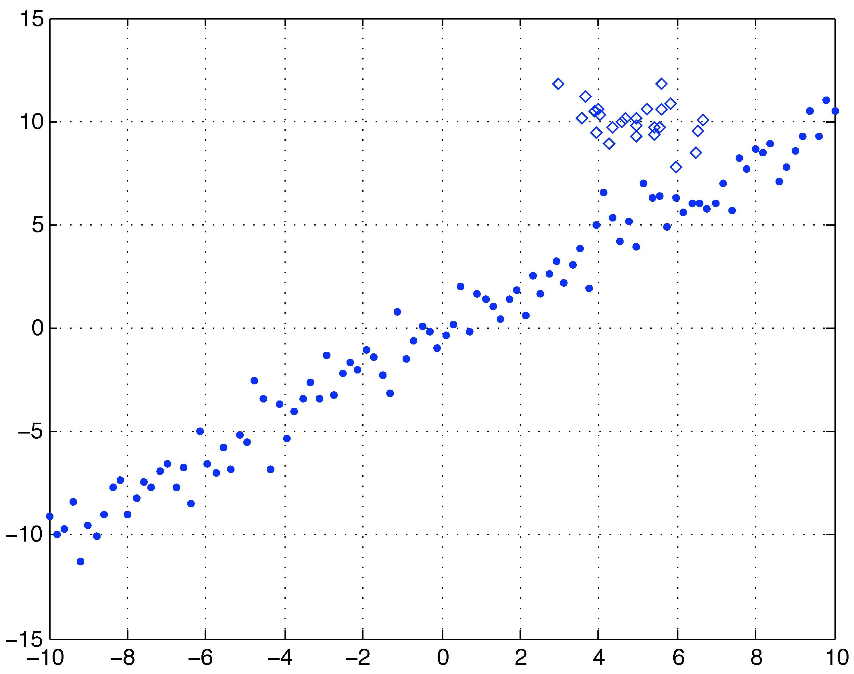
As a first toy example to investigate the properties of the proposed cost function H as compared to the Least Squares (LS) and Least Median of Squares alternatives, consider the data set depicted in Figure (1): there are 100 points depicted as dots having $x-$coordinates equally spaced in the range $[-10,10]$. The $y-$coordinates are computed as $y=x+ϵ$ being ϵ a Gaussian random noise of zero mean and unit variance. Moreover there are other 25 data points depicted with a diamond shape: these have $x-$coordinates normally distributed with mean 5 and unit variance, while their $y-$coordinates are normally distributed with mean 10 and unit variance. The total data set is made of the these 2 subsets, namely it contains 125 points that can be thought of as 100 values satisfying a linear model $y=x$ (with some noise), plus 25 outliers.

The reference model for the above described data set is

$$\mathbf{y}=\theta \mathbf{x}$$

being $\mathbf{y}$ and $\mathbf{x}\in {\mathbb{R}}^{125\times 1}$ known while $\theta \in \mathbb{R}$ is the unknown scalar to be estimated. Given the presence of the outliers, the LS estimate is expected to be biased with respect to the “real” value 1. Indeed its value results in

$${\widehat{\theta }}_{LS}=\frac{{\mathbf{x}}^T\mathbf{y}}{{\mathbf{x}}^T\mathbf{x}}=1.16.$$

(53)

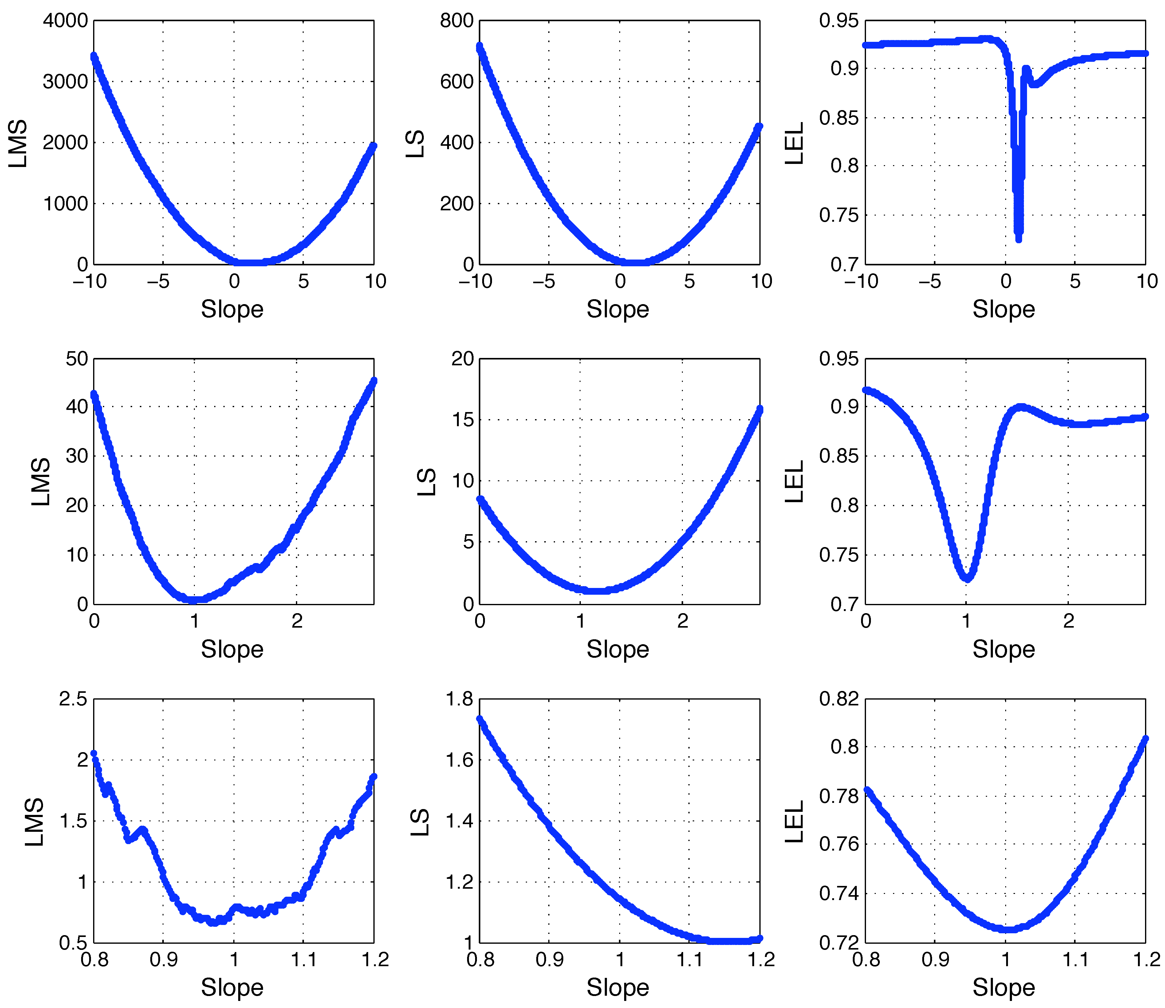
Given that the unknown parameter is a scalar, the LS, LMS and LEL cost functions can be easily plotted as functions of θ. The LMS, LS (normalized) and LEL cost functions are computed as

$$\begin{array}{ccc}\hfill f_{LMS}\left(\theta \right)& =& {\mathrm{med}}_i\left\{{(y_i-\theta x_i)}^2\right\}\hfill \end{array}$$

(54)

$$\begin{array}{ccc}\hfill f_{LS}\left(\theta \right)& =& \frac{{\sum }_i^N{\left(y_i-\theta x_i\right)}^2}{{\sum }_j^N{\left(y_j-{\widehat{\theta }}_{LS}{x}_j\right)}^2}\hfill \end{array}$$

(55)

$$\begin{array}{ccc}\hfill f_{LEL}\left(\theta \right)& =& -\frac{1}{logN}\sum _{i=1}^N\left(\frac{{(y_i-\theta x_i)}^2}{{\sum }_{j=1}^N{(y_j-\theta x_j)}^2}\right)log\left(\frac{{(y_i-\theta x_i)}^2}{{\sum }_{j=1}^N{(y_j-\theta x_j)}^2}\right)\hfill \end{array}$$

(56)

Figure 1. Linearly distributed data $y=x$ with zero mean unit variance noise (100 round dots) plus 25 outliers normally distributed around the point $(5,10)$. Refer to the text for details.

Figure 1. Linearly distributed data $y=x$ with zero mean unit variance noise (100 round dots) plus 25 outliers normally distributed around the point $(5,10)$. Refer to the text for details.

where ${med}_i\{·\}$ is the sample median over the set in argument and $N=125$. The LS cost $f_{LS}\left(\theta \right)$ in equation (55) is normalized such that $f_{LS}({\widehat{\theta }}_{LS})=1$ whereas the LEL cost function $f_{LEL}\left(\theta \right)$ in (56) is the H function of equation (42) except for checking if ${\sum }_{j=1}^N{(y_j-\theta x_j)}^2$ is null or not (unnecessary in practice). These cost functions are sampled in the range $\theta \in [-10,10]$ with ${10}^4$ equally spaced values of the slope θ: the resulting plots are depicted in Figure (2) at different zoom levels. As expected, the LS cost has a (unique) minimum in $1.16$. The LMS cost has a discontinuous and rather erratic behavior making it difficult to accurately determine where its minima are. The LEL cost function has a regular plot (the function is actually smooth in this case) and it appears to have a sharp local minimum in $\theta =1$. Notice that the LEL function has also a local minimum close to $\theta =2$ confirming the local nature of the proposed estimator. To explore the behavior of the proposed approach on a multidimensional problem, consider the following model:

$$y_i={\theta }_{r1}sin\left({\omega }_1{x}_i\right)+{\theta }_{r2}cos\left({\omega }_1{x}_i\right)+{\theta }_{r3}sin\left({\omega }_2{x}_i\right)+{\theta }_{r4}cos\left({\omega }_2{x}_i\right)+{\epsilon }_i$$

(57)

or, in vector notation,

$$\begin{array}{ccc}\hfill \mathbf{y}& =& G{\mathit{\theta }}_r+\mathit{\epsilon }\hfill \end{array}$$

(58)

$$\begin{array}{ccc}\hfill G& =& \left[\begin{array}{cccc}sin\left({\omega }_1{x}_1\right)& cos\left({\omega }_1{x}_1\right)& sin\left({\omega }_2{x}_1\right)& cos\left(\omega x_1\right)\\ ⋮& ⋮& ⋮& ⋮\\ sin\left({\omega }_1{x}_N\right)& cos\left({\omega }_1{x}_N\right)& sin\left({\omega }_2{x}_N\right)& cos\left(\omega x_N\right)\end{array}\right]\hfill \end{array}$$

(59)

Figure 2. LMS, LS and LEL costs as function of the line slope. Refer to the text for details.

Figure 2. LMS, LS and LEL costs as function of the line slope. Refer to the text for details.

where ${\omega }_1$ and ${\omega }_2$ are known, but ${\mathit{\theta }}_r$ is not. Assume that a data set $(\mathbf{y},\mathbf{x}):\mathbf{x},\mathbf{y}\in {\mathbb{R}}^{N\times 1}$ is available and that $\mathit{\epsilon }\in {\mathbb{R}}^{N\times 1}$ is a vector of zero mean, normally distributed noise (eventually with known covariance). The following numerical experiment (Case 1) is performed: the “real” value of the parameter vector ${\mathit{\theta }}_r$ is randomly generated (each component is the rounded value of a uniformly distributed number in the range $[-100,100]$) yielding ${\mathit{\theta }}_r={(63,2,11,-29)}^T$. The values of ${\omega }_1$ and ${\omega }_2$ are chosen to be ${\omega }_1=1$ and ${\omega }_2=2$ and the noise term $\mathit{\epsilon }$ is normally distributed (i.i.d.) with zero mean and variance equal to 10. The independent variable $\mathbf{x}$ is generated as a uniform ramp of $N={10}^4$ values in the range $[-10,10]$, whereas $\mathbf{y}$ is computed according to equation (58). Given these numerical values, the LS estimate of ${\mathit{\theta }}_r$ may be computed as ${\widehat{\mathit{\theta }}}_{LS}={\left(G^{T}G\right)}^{-1}{G}^T\mathbf{y}$ resulting in ${\widehat{\mathit{\theta }}}_{LS}={(62.92,2.03,11.02,-29.03)}^T$. The corresponding LEL estimate (Case 1) is computed according to its definition (46). In particular the minimization of the H function is performed 4 times starting from 4 different initialization values computed as in equations (50–51) with ${\mathit{\theta }}_0={\widehat{\mathit{\theta }}}_{LS}$. The minimization routine is the FMINSEARCH multidimensional unconstrained nonlinear minimization (Nelder-Mead) of Matlab (Version 7.8.0.347 (R2009a)). The results of these minimizations are summarized in Table 1: the first column refers to the values of $\mathit{\theta }$ used to initialize the minimization routine. The second column refers to the local minimum that was found and the third column refers to the value of H in such local minimum. Notice that the top element of the first column (case 1A) is ${\widehat{\mathit{\theta }}}_{LS}$. Also notice that cases 1C and 1D lead to the same local minimum and that the least value of H is obtained in case 1A. Nevertheless in all four cases the value of H is relatively high (recall that $H\in [0,1]$) and the differences among the four cases (in particular 1A, 1C and 1D) are extremely small, i.e., poorly significant. The plot of the $(\mathbf{x},\mathbf{y})$ data together with the LS and LEL fits (1A, 1B, 1C/D) are reported in Figure (3).

Table 1. LEL estimates: Case 1 (refer to text for details).

initial θ	final θ	final H	Case
${(62.92,2.03,11.02,-29.03)}^T$	${(62.15,2.38,11.89,-28.00)}^T$	0.9199	1A
${(-30.79,-0.64,30.65,-55.13)}^T$	${(26.69,-3.70,40.78,-19.82)}^T$	0.9287	1B
${(-3.93,59.24,-33.35,-17.04)}^T$	${(-32.94,54.63,-42.48,43.37)}^T$	0.9219	1C
${(2.27,37.60,52.48,27.47)}^T$	${(-32.94,54.63,-42.48,43.37)}^T$	0.9219	1D

Table 1. LEL estimates: Case 1 (refer to text for details).

initial θ	final θ	final H	Case
${(62.92,2.03,11.02,-29.03)}^T$	${(62.15,2.38,11.89,-28.00)}^T$	0.9199	1A
${(-30.79,-0.64,30.65,-55.13)}^T$	${(26.69,-3.70,40.78,-19.82)}^T$	0.9287	1B
${(-3.93,59.24,-33.35,-17.04)}^T$	${(-32.94,54.63,-42.48,43.37)}^T$	0.9219	1C
${(2.27,37.60,52.48,27.47)}^T$	${(-32.94,54.63,-42.48,43.37)}^T$	0.9219	1D

Figure 3. Case 1 data with LS and LEL fit. Refer to the text for details.

Figure 3. Case 1 data with LS and LEL fit. Refer to the text for details.

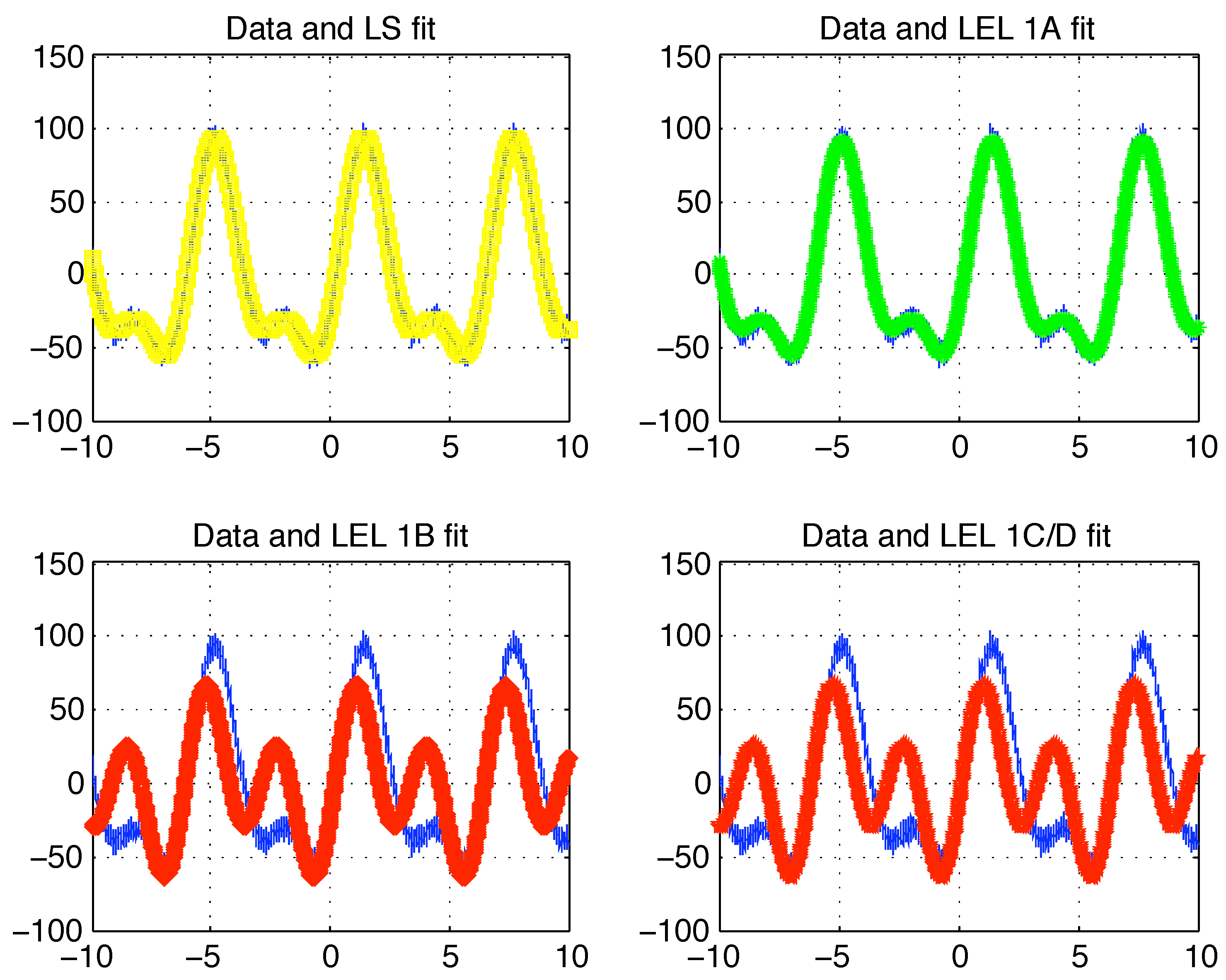
The LEL-1A estimate is very close to the LS one (that is very close to the real parameter vector ${\mathit{\theta }}_r$) and in Figure (3) the fitted data $G{\widehat{\mathit{\theta }}}_{LEL-1A}$ and $G{\widehat{\mathit{\theta }}}_{LS}$ appear to be almost perfectly overlapping with the original data $\mathbf{y}$ (first row in Figure (3)). To the contrary, the fitting behavior of the other two LEL estimates is clearly less accurate. A quantitative criteria to determine unambiguously which of the four (LS, LEL-1A, LEL-1B, LEL-1C/D) estimates is the “best” can be the value of the median of the fitting errors. More precisely, the median of the absolute fitting errors or of the squared fitting errors. These values are reported in Table 2.

Table 2. Median of fitting errors: Case 1 (refer to text for details).

Estimate	${\mathrm{med}}_i\{|y_i-{(G\widehat{\mathit{\theta }})}_i|\}$	${\mathrm{med}}_i\{{(y_i-{(G\widehat{\mathit{\theta }})}_i)}^2\}$	Case
${\widehat{\mathit{\theta }}}_{LS}$	$2.1719$	$4.7170$	LS
${\widehat{\mathit{\theta }}}_{LEL-1A}$	$2.2901$	$5.2444$	1A
${\widehat{\mathit{\theta }}}_{LEL-1B}$	$22.3232$	$498.33$	1B
${\widehat{\mathit{\theta }}}_{LEL-1C/D}$	$55.5248$	3083	1C/D

Table 2. Median of fitting errors: Case 1 (refer to text for details).

Estimate	${\mathrm{med}}_i\{|y_i-{(G\widehat{\mathit{\theta }})}_i|\}$	${\mathrm{med}}_i\{{(y_i-{(G\widehat{\mathit{\theta }})}_i)}^2\}$	Case
${\widehat{\mathit{\theta }}}_{LS}$	$2.1719$	$4.7170$	LS
${\widehat{\mathit{\theta }}}_{LEL-1A}$	$2.2901$	$5.2444$	1A
${\widehat{\mathit{\theta }}}_{LEL-1B}$	$22.3232$	$498.33$	1B
${\widehat{\mathit{\theta }}}_{LEL-1C/D}$	$55.5248$	3083	1C/D

The results summarized in Table 2 suggest that the LS estimate, in this case, should be preferred to the LEL one. To cross check this result, it may be useful to graphically inspect the plot of the sorted absolute values of the fitting errors as depicted in Figure (5).

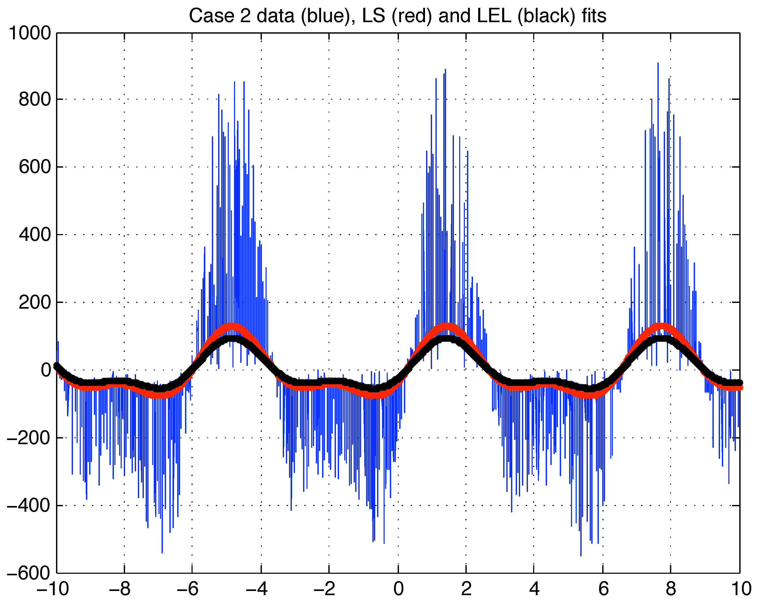
These results should not be surprising as in the given setting (no outliers and additive zero mean normally distributed noise) the LS is guaranteed to be the optimal estimator. Yet things change considerably if the data set $(\mathbf{x},\mathbf{y})$ is corrupted so that some of the data (a minority) will not satisfy the above hypothesis. Assume, for example, that a fraction of the available $\mathbf{y}$ values (say $10\%$) are multiplied by a random gain in the range $[0,10]$ (due to some data recording or communication problem, it does not really matter here). In particular this kind of corruption (Case 2) is generated taking exactly the same $\mathbf{y}$ vector of Case 1 and multiplying $10\%$ randomly selected components of $\mathbf{y}$ (i.e., 1000 randomly selected y values) each by a different random number uniformly distributed in the range $[0,10]$. The resulting data is plotted in Figure (4).

The LS estimate of $\mathit{\theta }$ based on this corrupted data (Case 2) results in ${\widehat{\mathit{\theta }}}_{LS}={(87.44,2.68,15.95,-39.96)}^T$ that appears to be significantly distant from the real value ${\mathit{\theta }}_r$ (and from the Case 1 LS estimate). The LEL estimate is computed exactly as described for Case 1, but using the new (Case 2) LS estimate as initialization value ${\widehat{\mathit{\theta }}}_0$.

The results are summarized in Table 3. Notice that the minimization routine always converges to the same value that appears to be very close to the real one. Moreover, the least value of H is significantly smaller than in Case 1 suggesting that the distribution of the relative squared residuals has a smaller dispersion than in Case 1. The plots of the LS fit, the LEL fit and the case 2 data is depicted in Figure (6).

Figure 4. Case 2 corrupted data (red dots) and original data (solid blue line).

Figure 4. Case 2 corrupted data (red dots) and original data (solid blue line).

Figure 5. Case 1 sorted LS and LEL fitting errors in absolute value.

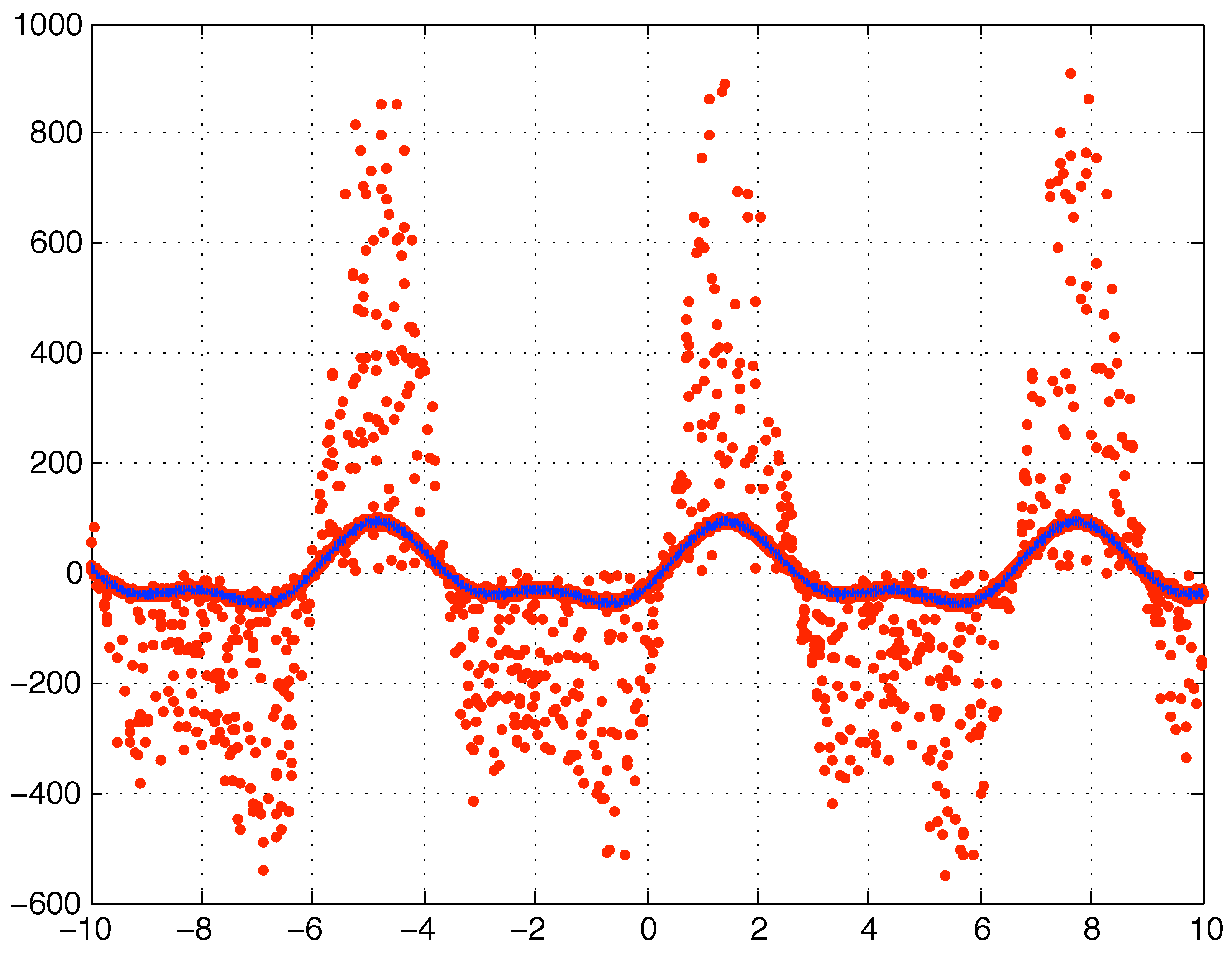
Figure 5. Case 1 sorted LS and LEL fitting errors in absolute value.

Figure 6. Case 2 data (blue), LS fit (red) and LEL fit (black).

Figure 6. Case 2 data (blue), LS fit (red) and LEL fit (black).

Table 3. LEL estimates: Case 2 (refer to text for details).

initial θ	final θ	final H	Case
${(87.44,2.68,15.95,-39.96)}^T$	${(64.18,2.46,10.66,-28.87)}^T$	0.6455	2A
${(27.44,-21.20,-88.03,23.49)}^T$	${(64.18,2.46,10.66,-28.87)}^T$	0.6455	2B
${(-33.04,0.03,-33.13,-85.53)}^T$	${(64.18,2.46,10.66,-28.87)}^T$	0.6455	2C
${(3.66,95.12,-20.06,6.38)}^T$	${(64.18,2.46,10.66,-28.87)}^T$	0.6455	2D

Table 3. LEL estimates: Case 2 (refer to text for details).

initial θ	final θ	final H	Case
${(87.44,2.68,15.95,-39.96)}^T$	${(64.18,2.46,10.66,-28.87)}^T$	0.6455	2A
${(27.44,-21.20,-88.03,23.49)}^T$	${(64.18,2.46,10.66,-28.87)}^T$	0.6455	2B
${(-33.04,0.03,-33.13,-85.53)}^T$	${(64.18,2.46,10.66,-28.87)}^T$	0.6455	2C
${(3.66,95.12,-20.06,6.38)}^T$	${(64.18,2.46,10.66,-28.87)}^T$	0.6455	2D

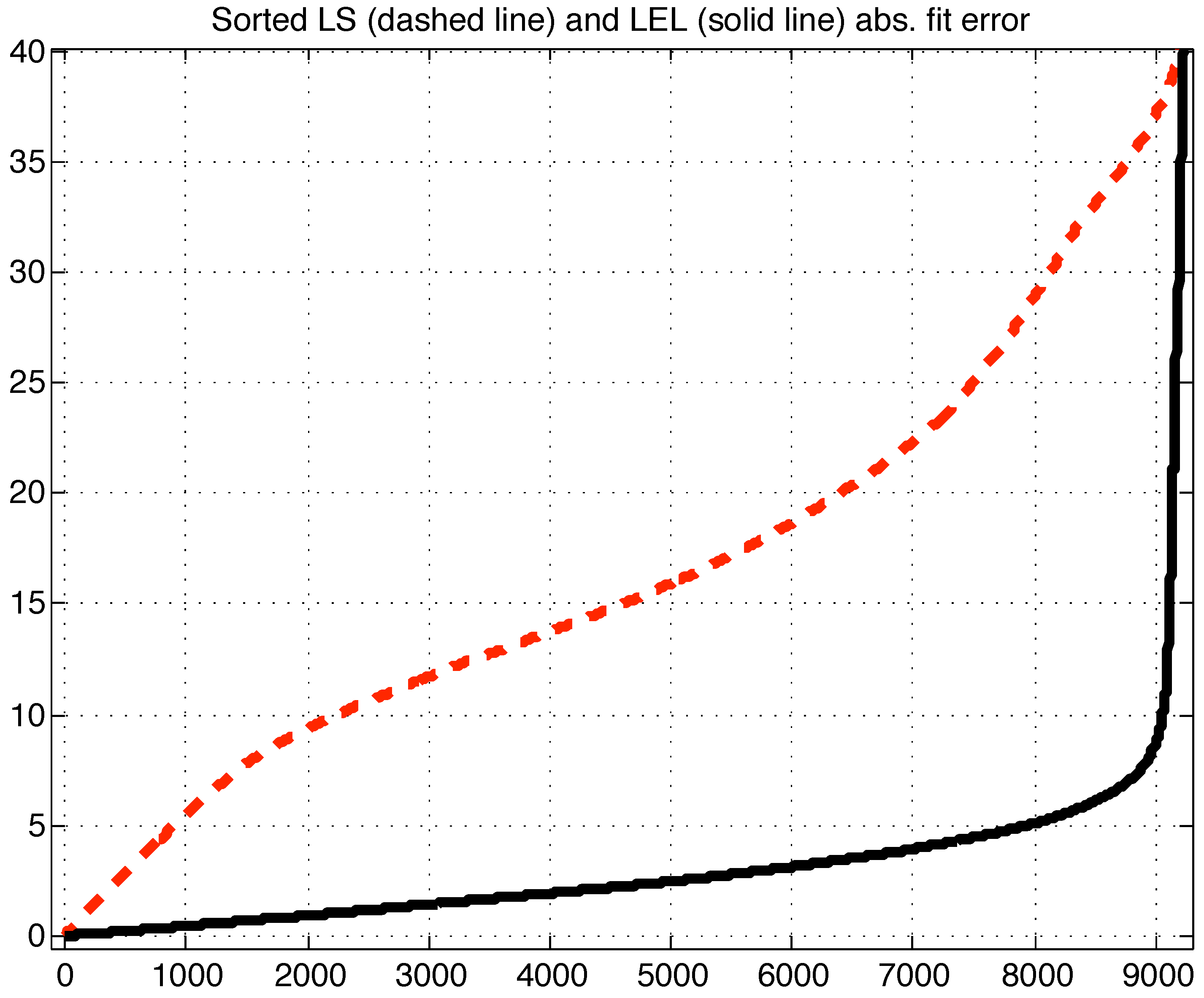
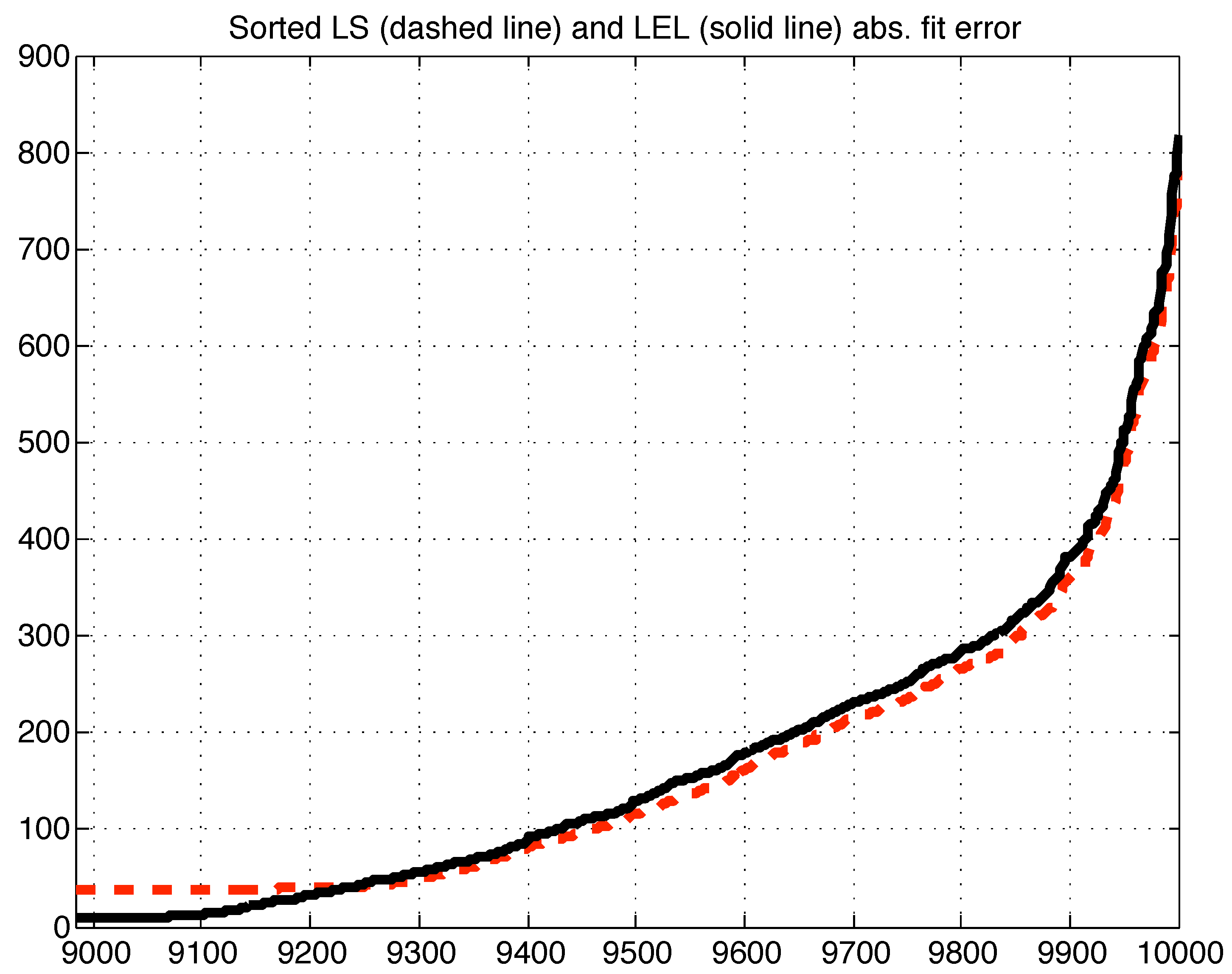
As for Case 1, based on the only plots of the fitted data, it is not obvious which model is performing better. Yet in terms of the median of the absolute values of the residuals (Table 4), the LEL estimate is certainly to be preferred. Indeed the plot of the sorted absolute residuals in Figure (7) and Figure (8) reveals that the great majority (about $90\%$) of the data is significantly closer to the LEL fit rather than the LS fit.

The Case 2 experiment has been repeated 100 times with different values of ${\mathit{\theta }}_r$, namely each time its components were rounded values of uniformly distributed numbers in the range $[-100,100]$. In each of the 100 iterations all the random variables used were different realizations. Each of the 100 iterations gave similar results to the ones described, i.e., a LEL estimate was computed that had lower median of absolute residuals with respect to the LS estimate and was closer to the real parameter vector. As for computational effort, the minimization of the H function was performed with the FMINSEARCH multidimensional unconstrained nonlinear minimization (Nelder-Mead) of Matlab (Version 7.8.0.347 (R2009a)). The Matlab code was not optimized. The computer platform was an Apple Laptop with a 2.16 GHz Intel Core 2 Duo processor, 2 GB RAM, running the MAC OS X Version 10.5.8 operating system. The CPU time required for minimizing the H function resulted to be on average $(1.41\pm 0.19)$[s] where the error was computed as the sample standard deviation of all the iterations. Recalling that the number of data points was always $N={10}^4$ this result is rather interesting as it suggests that the proposed method can be eventually employed for on line applications, at least for models of comparable size.

Figure 7. First 9000 sorted LS (dashed line) and LEL (solid line) absolute fitting errors (i.e., residuals).

Figure 7. First 9000 sorted LS (dashed line) and LEL (solid line) absolute fitting errors (i.e., residuals).

Table 4. Median of fitting errors: Case 2.

Estimate	${\mathrm{med}}_i\left\{\right|y_i-{(G\widehat{\mathit{\theta }})}_i\left|\right\}$	Case
${\widehat{\mathit{\theta }}}_{LS}$	$15.91$	LS
${\widehat{\mathit{\theta }}}_{LEL}$	$2.46$	2A/B/C/D

Table 4. Median of fitting errors: Case 2.

Estimate	${\mathrm{med}}_i\left\{\right|y_i-{(G\widehat{\mathit{\theta }})}_i\left|\right\}$	Case
${\widehat{\mathit{\theta }}}_{LS}$	$15.91$	LS
${\widehat{\mathit{\theta }}}_{LEL}$	$2.46$	2A/B/C/D

As a final numerical experiment to evaluate the performance of the proposed method in comparison to the LMS technique, consider the following model:

$$\mathbf{y}=G\mathit{\theta }$$

(60)

being $\mathbf{y}\in {\mathbb{R}}^{75\times 1}$, $\mathit{\theta }\in {\mathbb{R}}^{3\times 1}$ and $G=\left[{\mathbf{x}}_1{\mathbf{x}}_2{\mathbf{x}}_3\right]\in {\mathbb{R}}^{75\times 3}$. The $\mathbf{y},{\mathbf{x}}_1,{\mathbf{x}}_2$ and ${\mathbf{x}}_3$ values are given by the Hawkins - Bradu - Kass data set [1] (Chapter 3, section 3) available in electronic format (together with all the other data sets used in [1]) from the University of Cologne Statistical Resources http://www.uni-koeln.de/themen/statistik/index.e.html (follow the links DATA and then Cologne Data Sets). The first 10 values of this artificially generated data set correspond to bad leverage points, i.e. outliers that can significantly affect the LS estimate (refer to [1] for more details). Points 11, 12, 13 and 14 are outliers in ${\mathbf{x}}_i$, namely they lay far from the bulk of the rest of the data in ${\mathbf{x}}_i$ space, but their y values agree with the model. A LEL estimate of $\mathit{\theta }$ is computed by minimizing the corresponding H function from three different initialization values computed as in equations (50–51) using the Least Squares estimate ${\widehat{\mathit{\theta }}}_{LS}$ as a ${\widehat{\mathit{\theta }}}_0$. The three so computed LEL estimates are labelled as A, B and C. Their values are listed in Table 5.

Figure 8. Last 1000 sorted LS (dashed line) and LEL (solid line) absolute fitting errors (i.e., residuals).

Figure 8. Last 1000 sorted LS (dashed line) and LEL (solid line) absolute fitting errors (i.e., residuals).

Table 5. Hawkins–Bradu–Kass data set analysis.

Estimate	${\mathrm{med}}_i\{{(y_i-{(G\widehat{\mathit{\theta }})}_i)}^2\}$	H value
${\widehat{\mathit{\theta }}}_{LS}={(0.08,-0.36,0.44)}^T$	$0.68$	$0.6532$
${\widehat{\mathit{\theta }}}_{LEL-A/B}={(-0.33,0.33,0.23)}^T$	$0.53$	$0.4290$
${\widehat{\mathit{\theta }}}_{LEL-C}={(-0.0043,0.05,-0.05)}^T$	$0.31$	$0.5600$

Table 5. Hawkins–Bradu–Kass data set analysis.

Estimate	${\mathrm{med}}_i\{{(y_i-{(G\widehat{\mathit{\theta }})}_i)}^2\}$	H value
${\widehat{\mathit{\theta }}}_{LS}={(0.08,-0.36,0.44)}^T$	$0.68$	$0.6532$
${\widehat{\mathit{\theta }}}_{LEL-A/B}={(-0.33,0.33,0.23)}^T$	$0.53$	$0.4290$
${\widehat{\mathit{\theta }}}_{LEL-C}={(-0.0043,0.05,-0.05)}^T$	$0.31$	$0.5600$

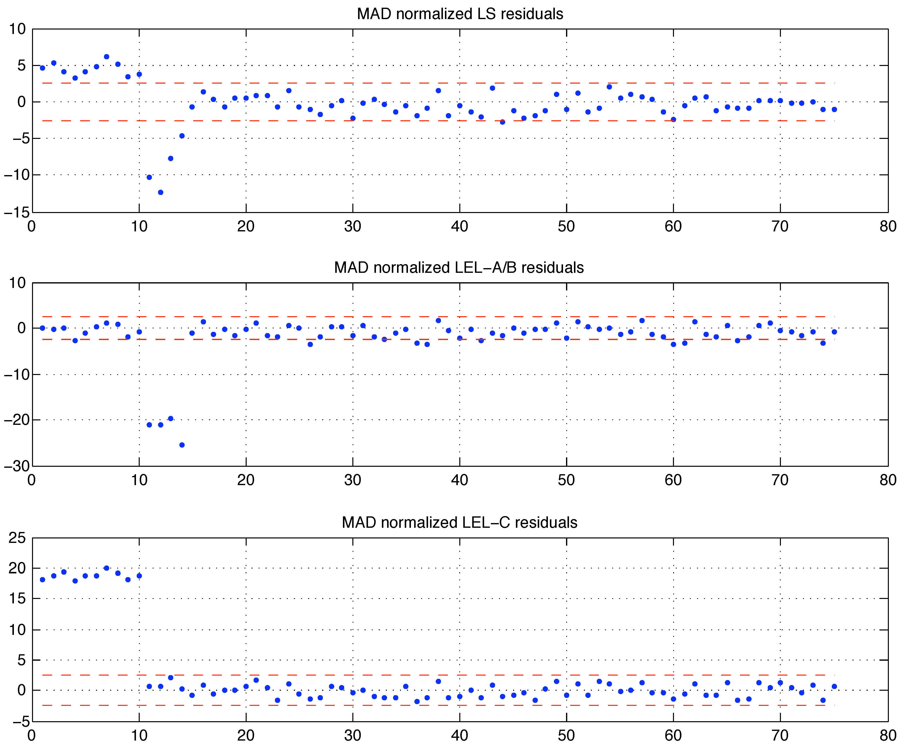
The A and B estimates coincide and correspond to the least value of H among the three. Hence the best (local) LEL estimate of $\mathit{\theta }$ is to be considered ${\widehat{\mathit{\theta }}}_{LEL-A/B}$. Nevertheless, interestingly this estimate does not correspond to the least value of the median of squares cost. The ${\widehat{\mathit{\theta }}}_{LEL-C}$ estimate performs better in terms of the median of squares cost criteria. For a graphical interpretation of these results, refer to Figure (9) where the residuals, scaled by their median absolute deviation MAD (21) scale estimate, are depicted. Comparing the bottom plot in Figure (9) with the equivalent plot for the LMS estimate in [1] (p. 95), one can arguably conclude that the ${\widehat{\mathit{\theta }}}_{LEL-C}$ estimate is (very) close to the LMS one. This shows that the LEL and LMS criteria differ and should not be considered equivalent, although in spirit both are defined so that the residual scatter is somehow minimized. The Hawkins–Bradu–Kass example also shows that the LEL estimate can be affected by the presence of bad leverage points (outliers): notice that the central plot in Figure (9) reveals how the (best) LEL estimate (A/B) accommodates the 10 bad leverage points within the fit and excludes the four ${\mathbf{x}}_i$-space outliers 11, 12, 13 and 14. Although from the LEL criteria perspective one could also argue that the first 10 points are not outliers (or bad leverage points), whereas the following 4 are. Indeed the very definition of outlying data should be given according to a fitting criteria. The interpretation of similar results without an a priori agreement on the definition of outlier will always be debatable.

Figure 9. LS and LEL residuals of the Hawkins - Bradu - Kass data set fitting. The dashed lines indicate the $\pm 2.5$ values.

Figure 9. LS and LEL residuals of the Hawkins - Bradu - Kass data set fitting. The dashed lines indicate the $\pm 2.5$ values.

6. Conclusions

A novel prediction error method for robust parameter identification in the presence of outlying data has been presented. The approach builds on minimizing a cost function inspired by the concept of (Gibbs) entropy although the probabilistic or information theoretic meaning of entropy is not explicitly involved. The function to be minimized inherits the smoothness properties of the data model, hence if the model is sufficiently well behaved, any off-the-shelf unconstraint numerical minimization routine can be exploited. Although the asymptotical breakdown point of the algorithm is not any better than standard Least Squares, numerical examples were provided showing an excellent finite sample behavior. The function to be minimized may have multiple minima, hence the proposed approach is structurally local in nature. A simple heuristic method to select a family of initialization values for the local minimization has been suggested and tested on several examples. Potential outlying data can be identified by analyzing the (sorted) plot of the absolute (or squared) residuals.

One of the significant properties of the proposed method is relative to the low computational effort required to compute the parameter estimate; such property may be exploited in online applications. As an example, consider sensor signal processing in robotics or automatic controls. Assume that range or imaging data are acquired by a robot or a vehicle and that a set of features needs to be extracted from the data online. Typical examples may include sonar data acquired by marine or areal vehicles or images acquired by any moving robot equipped with a computer vision system. If a reliable estimate ${\widehat{\mathit{\theta }}}_k$ of the features is known at time k, it is often a reasonable assumption that they will be “approximately close” to ${\widehat{\mathit{\theta }}}_k$ at time $k+1$. In this case, the local nature of the LEL estimator may not be a serious issue, in the sense that at time $k+1$ one may estimate ${\widehat{\mathit{\theta }}}_{k+1}$ through the proposed LEL method using ${\widehat{\mathit{\theta }}}_k$ as the initialization value. Notice that the standard implementation of many alternative robust methods as RANSAC, the Hough transform, LMS or M-estimators would most probably be much more demanding from a computational point of view. Ongoing work is in progress to test the use of the LEL approach with experimental data, in particular for the identification of planes from $3D$ data acquired by a robot using a range camera (Figure (10)).

Figure 10. $3D$ range camera image of an office with LEL based detected (in red) wall.

Figure 10. $3D$ range camera image of an office with LEL based detected (in red) wall.

References

- Rousseeuw, P.J.; Leroy, A.M. Robust Regression and Outlier Detection; John Wiley & Sons, Inc.: Hoboken, NJ, USA, 2003. [Google Scholar]
- Huber, P.J. Robust Statistics; John Wiley & Sons, Inc.: New York, NY, USA, 1981. [Google Scholar]
- Pronzato, L.; Thierry, E. A minimum-entropy estimator for regression problems with unknown distribution of observation errors. Research Report 00-08. Laboratoire d’Informatique, Signaux et Systèmes I3S - UMR6070 - UNSA CNRS: Sophia-Antipolis, France, 2000. Available online: http://www.i3s.unice.fr/%7Epronzato/biblio.html (accessed on 1 October 2009).
- Wolsztynski, E.; Thierry, E.; Pronzato, L. Minimum-Entropy Estimation in Semi-Parametric Models. Signal Process. 2005, 85, 937–949. [Google Scholar]
- Ta, M.; DeBrunner, V. Minimum Entropy Estimation as a Near Maximum-Likelihood Method and Its Application in System Identification with Non-Gaussian Noise. In Proceedings of ICASSP ’04 - IEEE International Conference on Acoustics, Speech, and Signal Processing, Montreal, QC, Canada, 17-21 May 2004; Volume 2, pp. 545–548.
- Steele, J.M.; Steiger, W.L. Algorithms and Complexity for Least Median of Squares Regression. Discrete Appl. Math. 1986, 14, 93–100. [Google Scholar]
- Stromberg, A.J. Computing the Exact Least Median of Squares Estimate and Stability Diagnostics in Multiple Linear Regression. SIAM J. Sci. Comput. 1993, 14, 1289–1299. [Google Scholar] [CrossRef]
- He, X.; Portnoy, S. Reweighted LS Estimators Converge at the Same Rate as the Initial Estimator. Ann. Stat. 1992, 20, 2161–2167. [Google Scholar] [CrossRef]
- Gervini, D.; Yohai, V. A Class of Robust and Fully Efficient Regression Estimators. Ann. Stat. 2002, 30, 583–616. [Google Scholar] [CrossRef]
- Agostinelli, C.; Markatou, M. A One-step Robust Estimator for Regression Based on the Weighted Likelihood Reweighting Scheme. Stat. Probabil. Lett. 1998, 37, 341–350. [Google Scholar] [CrossRef]
- Bishop, C.M. Pattern Recognition and Machine Learning; Springer: New York, NY, USA, 2006. [Google Scholar]
- Luengo Hendriks, C.L.; van Ginkel, M.; Verbeek, P.W.; van Vliet, L.J. The Generalized Radon Transform: Sampling, Accuracy and Memory Considerations. Pattern Recogn. 2005, 38, 2494–2505. [Google Scholar] [CrossRef]
- Fischler, M.A.; Bolles, R.C. Random Sample Consensus: A Paradigm for Model Fitting with Applications to Image Analysis and Automated Cartography. Commun. ACM 1981, 24, 381–395. [Google Scholar] [CrossRef]
- Golan, A.; Kitamura, Y. Information and Entropy Econometrics - A Volume in Honor of Arnold Zellner. J. Econometrics 2007, 138, 379–586. [Google Scholar] [CrossRef]
- Golan, A.; Judge, G.G.; Miller, D. Maximum Entropy Econometrics: Robust Estimation with Limited Data; John Wiley & Sons Inc.: Chichester, UK, 1996. [Google Scholar]
- Ciavolino, E.; Dahlgaard, J.J. Simultaneous equation Model Based on the Generalized Maximum Entropy for Studying the Effect of Management Factors on Enterprise Performance. J. Appl. Stat. 2009, 36, 801–815. [Google Scholar] [CrossRef]
- Poljak, B.T.; Tsypkin, J.A.Z. Robust identification. Automatica 1980, 16, 53–63. [Google Scholar] [CrossRef]
- Bai, E-W. An Optimization Based Robust Identification Algorithm in the Presence of Outliers. J. Global Optim. 2002, 23, 195–211. [Google Scholar] [CrossRef]
- Cover, T.M.; Thomas, J.A. Elements of Information Theory; John Wiley & Sons, Inc.: New York, NY, USA, 1991. [Google Scholar]
- Indiveri, G. Notes on an Entropy-like Method for Robust Parameter Identification. Technical Report No. 17. School of Engineering and Science, Jacobs University Bremen: Bremen, Germany, 2008. Available online: http://www.jacobs-university.de/research/reports/ (Accessed on 1 October 2009).
© 2009 by the authors. Licensee Molecular Diversity Preservation International, Basel, Switzerland. This article is an open-access article distributed under the terms and conditions of the Creative Commons Attribution license http://creativecommons.org/licenses/by/3.0/.
Share and Cite
MDPI and ACS Style
Indiveri, G. An Entropy-Like Estimator for Robust Parameter Identification. Entropy 2009, 11, 560-585. https://doi.org/10.3390/e11040560
AMA Style
Indiveri G. An Entropy-Like Estimator for Robust Parameter Identification. Entropy. 2009; 11(4):560-585. https://doi.org/10.3390/e11040560
Chicago/Turabian StyleIndiveri, Giovanni. 2009. "An Entropy-Like Estimator for Robust Parameter Identification" Entropy 11, no. 4: 560-585. https://doi.org/10.3390/e11040560