Article

Simulation Study of Direct Causality Measures in Multivariate Time Series

1
Department of Economics, University of Macedonia, Egnatias 156, 54006, Thessaloniki, Greece
2
University of Strasbourg, BETA, University of Paris 10, Economix, ISC-Paris, Ile-de-France, France
3
Faculty of Engineering, Aristotle University of Thessaloniki, University Campus, 54124, Thessaloniki, Greece
4
Faculty of Economics, Department of Economics and Econometrics, University of Amsterdam, Valckenierstraat 65-67, 1018 XE, Amsterdam, The Netherlands
*
Author to whom correspondence should be addressed.
Entropy 2013, 15(7), 2635-2661; https://doi.org/10.3390/e15072635
Submission received: 28 March 2013 / Revised: 5 June 2013 / Accepted: 27 June 2013 / Published: 4 July 2013
(This article belongs to the Special Issue Transfer Entropy)

Abstract

:
Measures of the direction and strength of the interdependence among time series from multivariate systems are evaluated based on their statistical significance and discrimination ability. The best-known measures estimating direct causal effects, both linear and nonlinear, are considered, i.e., conditional Granger causality index (CGCI), partial Granger causality index (PGCI), partial directed coherence (PDC), partial transfer entropy (PTE), partial symbolic transfer entropy (PSTE) and partial mutual information on mixed embedding (PMIME). The performance of the multivariate coupling measures is assessed on stochastic and chaotic simulated uncoupled and coupled dynamical systems for different settings of embedding dimension and time series length. The CGCI, PGCI and PDC seem to outperform the other causality measures in the case of the linearly coupled systems, while the PGCI is the most effective one when latent and exogenous variables are present. The PMIME outweighs all others in the case of nonlinear simulation systems.
Classification:
PACS 05.45.Tp 05.45.-a 02.70.-c

1. Introduction

The quantification of the causal effects among simultaneously observed systems from the analysis of time series recordings is essential in many scientific fields, ranging from economics to neurophysiology. Estimating the inter-dependence among the observed variables provides valuable knowledge about the processes that generate the time series. Granger causality has been the leading concept for the identification of directional interactions among variables from their time series, and it has been widely used in economics [1]. However, the last few years, it has become popular also in many different fields, e.g., for the analysis of electroencephalograms.
The mathematical formulation of linear Granger causality is based on linear regression modeling of stochastic processes. Many modifications and extensions of the Granger causality test have been developed; see e.g., [2,3,4,5,6,7]. Most of the non-causality tests, built on the Granger causality concept and applied in economics, are therefore based on the modeling of the multivariate time series. Despite the success of these strategies, the model-based methods may suffer from the shortcomings of model mis-specification.
The majority of the measures determining the interrelationships among variables that have been developed so far are for bivariate data, e.g., state-space based techniques [8,9], information measures [10,11,12] and techniques based on the concept of synchronization [13,14].
Bivariate causality tests may erroneously detect couplings when two variables are conditionally independent. To address this, techniques accounting for the effect of the confounding variables have been introduced, termed direct causality measures, which are more appropriate when dealing with multivariate time series [15,16,17]. Direct causality methods emerged as extensions of bivariate Granger causality. For example, the Granger causality index (GCI), implementing the initial idea for two variables in the time domain, has been extended to the conditional and partial Granger causality index (CGCI and PGCI) [2,18]. Directed coherence (DC) was introduced in the frequency domain, and being a bivariate measure, it cannot discriminate between direct and indirect coupling. The direct transfer function (DTF) is similarly defined as DC [19]. The partial directed coherence (PDC) is an extension of DC to multivariate time series measuring only the direct influences among the variables [20]. Similarly, direct Directed Transfer Function (dDTF) modified DTF to detect only direct information transfer [21].
Information theory sets a natural framework for non-parametric methodologies of several classes of statistical dependencies. Several techniques from information theory have been used in the last few years for the identification of causal relationships in multivariate systems, and the best known is transfer entropy (TE) [11]. Test for causality using the TE has also been suggested [22]. However, the TE is, again, bivariate and its natural extension to account for the presence of confounding variables has been recently introduced, namely, the partial TE (PTE), under different estimating schemes, using bins [23], correlation sums [24] and nearest neighbors [25]. The TE and PTE are actually expressions of conditional mutual information, and with this respect, an improved version of TE making use of a properly restricted non-uniform state space reconstruction was recently developed, termed mutual information on mixed embedding (MIME) [26]. Later, a similar approach to TE/PTE was implemented, which takes into consideration the conditional entropy [27]. Recently MIME was extended for multivariate time series to the partial MIME (PMIME) [28]. Other coupling methods have also been suggested, such as Renyi’s information transfer [29]. In a different approach, the TE has been defined on rank vectors instead of sample vectors, called the symbolic transfer entropy (STE) [30], and, respectively, to the multivariate case termed partial STE (PSTE) (for a correction of STE and PSTE, see, respectively, [31,32]).
Most comparative works on the effectiveness of causality measures concentrate on bivariate tests, e.g., [33,34,35,36], while some works evaluating multivariate methodologies include only model-based tests, see, e.g., [37,38,39], or compare direct and indirect causality measures, e.g., [36,40].
In this work, we compare model-based methods, both in the time and frequency domain, and information theoretic multivariate causality measures that are able to distinguish between direct and indirect causal effects. We include in the study most of the known direct causality measures of these classes, i.e., CGCI and PGCI (linear in time domain), PDC (linear in frequency domain), PTE, PSTE and PMIME (from information theory). The statistical significance of the test statistics is assessed with resampling methods, bootstraps or randomization tests using appropriate surrogates, whenever it is not theoretically known.
The structure of the paper is as follows. The multivariate causality measures considered in this study are presented in Section 2. The statistical significance of the coupling measures is assessed on simulated systems. The simulation systems and the setup of the simulation study are presented in Section 3, while the results of this study and the performance of the causality measures are discussed in Section 4. Finally, the conclusions are drawn in Section 5.

2. Direct Causality Measures

Let { x 1 , t , , x K , t } , t = 1 , , n , denote a K-variate time series, consisting of K simultaneously observed variables, X 1 , , X K , belonging to a dynamical system or representing respective subsystems of a global system. The reconstructed vectors of each X i are formed as x i , t = ( x i , t , x i , t τ i , , x i , t ( m i 1 ) τ i ) , where t = 1 , , n , n = n max i { ( m i 1 ) τ i } , and m i and τ i are, respectively, the reconstruction parameters of embedding dimension and time delay for X i . The notation, X 2 X 1 , denotes the Granger causality from X 2 to X 1 , while X 2 X 1 | Z denotes the direct Granger causality from X 2 to X 1 , accounting for the presence of the other (confounding) variables, i.e., Z = { X 3 , , X K } . The notation of Granger causality for other pairs of variables is analogous.
Almost all of the causality measures require the time series be stationary, i.e., their mean and variance do not change over time. If the time series are non-stationary, then the data should be pre-processed, e.g., for time series that are non-stationary in mean, one can apply the measures on the first or higher order differences. Different transformations are needed in case of non-stationary data in variance or co-integrated time series.

2.1. Conditional Granger Causality Index

Granger causality is based on the concept that if the value of a time series, X 1 , to be predicted is improved by using the values of X 2 , then we say that X 2 is driving X 1 . A vector autoregressive model (VAR) in two variables and of order P, fitted to the time series, { x 1 , t } , is:
x 1 , t + 1 = j = 0 P 1 a 1 , j x 1 , t j + j = 0 P 1 b 1 , j x 2 , t j + ϵ 1 , t + 1
where a 1 , j , b 1 , j are the coefficients of the model and ϵ 1 the residuals from fitting the model with variance s 1 U 2 . The model in Equation (1) is referred to as the unrestricted model, while the restricted model is obtained by omitting the terms regarding the driving variable [the second sum in Equation (1)] and has residual variance, s 1 R 2 . According to the concept of Granger causality, the variable, X 2 , Granger causes X 1 if s 1 R 2 > s 1 U 2 [1]. The magnitude of the effect of X 2 on X 1 is given by the Granger Causality Index (GCI), defined as:
GCI X 2 X 1 = ln ( s 1 R 2 / s 1 U 2 )
Considering all K variables, the unrestricted model for X 1 is a VAR model in K variables and involves the P lags of all K variables [K sum terms instead of two in Equation (1)]; the restricted model will have all but the P lags of the driving variable, X 2 . Likewise, the conditional Granger causality index (CGCI) is:
CGCI X 2 X 1 | Z = ln ( s 1 R 2 / s 1 U 2 )
where s 1 U 2 and s 1 R 2 are the residual variances for the unrestricted and restricted model defined for all K variables.
A parametric significance test for GCI and CGCI can be conducted for the null hypothesis that variable X 2 is not driving X 1 , making use of the F-significance test for all P coefficients, b 1 , j [41]. When we want to assess collectively the causal effects among all pairs of the K variables, a correction for multiple testing should be performed, e.g., by means of the false discovery rate [42].
The order, P, of the VAR model is usually chosen using an information criterion, such as the Akaike Information Criterion (AIC) [43] and the Bayesian Information Criterion (BIC) [44]. The estimation of the coefficients of the VAR models and the residual variances of the models are described analytically in [45].

2.2. Partial Granger Causality Index

The partial Granger causality index (PGCI) is associated with the concept of Granger causality and partial correlation [18]. The PGCI addresses the problem of exogenous inputs and latent variables. The intuition is that the influence of exogenous and/or latent variables on a system will be reflected by correlations among the residuals of a VAR model of the measured variables. Thus, in the PGCI, one makes use of the residual covariance matrix of the VAR unrestricted and restricted model, denoted Σ and ρ, respectively, and not only of the residual variance of the response variable, X 1 , s 1 U 2 and s 1 R 2 , subsequently. For example, for X 2 X 1 | X 3 , denoting the components of Σ as Σ i j , i , j = 1 , 2 , 3 and the components of ρ as ρ i j , i , j = 1 , 2 , the PGCI is given as:
PGCI X 2 X 1 | X 3 = ln ρ 11 ρ 12 ρ 22 1 ρ 21 Σ 11 Σ 13 Σ 33 1 Σ 31
Note that Σ 11 = s 1 U 2 and ρ 11 = s 1 R 2 . The PGCI constitutes an improved estimation of the direct Granger causality as compared to the CGCI when the residuals of the VAR models are correlated; otherwise, it is identical to the CGCI. The estimation procedure for the PGCI is described analytically in [18].

2.3. Partial Directed Coherence

The partial directed coherence (PDC) is related to the same VAR model as the CGCI, but is defined in the frequency domain [20]. Denoting the K × K matrix of the Fourier transform of the coefficients of the VAR model in K variables and order P by A ( f ) , the PDC from X 2 to X 1 at a frequency f is given by [20]:
PDC X 2 X 1 | Z ( f ) = | A 1 , 2 ( f ) | k = 1 K | A k , 2 ( f ) | 2
where A i , j ( f ) is the component at the position, ( i , j ) , in the matrix, A ( f ) . PDC X 2 X 1 | Z ( f ) provides a measure for the directed linear influence of X 2 on X 1 at frequency, f, conditioned on the other K 2 variables in Z and takes values in the interval, [ 0 , 1 ] . The PDC X 2 X 1 ( f ) is computed at each frequency, f, within an appropriate range of frequencies. Parametric inference and significance tests for PDC have been studied in [46,47].

2.4. Partial Transfer Entropy

The transfer entropy (TE) is a nonlinear measure that quantifies the amount of information explained in X 1 at h steps ahead from the state of X 2 , accounting for the concurrent state of X 1 [11]. The TE is given here in terms of entropies. For a discrete variable, X (scalar or vector), the Shannon entropy is H ( X ) = p ( x i ) ln p ( x i ) , where p ( x i ) is the probability mass function of variable, X, at the value, x i . Further, the TE is expressed as:
TE X 2 X 1 = I ( x 1 , t + h ; x 2 , t | x 1 , t ) = H ( x 1 , t + h | x 1 , t ) H ( x 1 , t + h | x 2 , t , x 1 , t ) = H ( x 2 , t , x 1 , t ) H ( x 1 , t + h , x 2 , t , x 1 , t ) + H ( x 1 , t + h , x 1 , t ) H ( x 1 , t )
The first equality is inserted to show that the TE is equivalent to the conditional mutual information (CMI), where I ( X , Y ) = H ( X ) + H ( Y ) H ( X , Y ) is the mutual information (MI) of two variables, X and Y. The time horizon, h, is introduced here instead of the single time step, originally used in the definition of TE.
The partial transfer entropy (PTE) is the extension of the TE designed for the direct causality of X 2 to X 1 conditioning on the remaining variables in Z
PTE X 2 X 1 | Z = H ( x 1 , t + h | x 1 , t , z t ) H ( x 1 , t + h | x 2 , t , x 1 , t , z t )
The entropy terms of PTE are estimated here using the k-nearest neighbors method [48].

2.5. Symbolic Transfer Entropy

The symbolic transfer entropy (STE) is the continuation of the TE estimated on rank-points formed by the reconstructed vectors of the variables [30]. For each vector, x 2 , t , the ranks of its components assign a rank-point, x ^ 2 , t = [ r 1 , r 2 , , r m 2 ] , where r j { 1 , 2 , , m 2 } for j = 1 , , m 2 . Following this sample-point to rank-point conversion, the sample, x 1 , t + h , in Equation (7) is taken as the rank point at time, t + h , x ^ 1 , t + h , and STE is defined as:
STE X 2 X 1 = H ( x ^ 1 , t + h | x ^ 1 , t ) H ( x ^ 1 , t + h | x ^ 2 , t , x ^ 1 , t )
where the entropies are computed based on the rank-points.
In complete analogy to the derivation of the PTE from the TE, the partial symbolic transfer entropy (PSTE) extends the STE for multivariate time series and is expressed as:
PSTE X 2 X 1 | Z = H ( x ^ 1 , t + h | x ^ 1 , t , z ^ t ) H ( x ^ 1 , t + h | x ^ 2 , t , x ^ 1 , t , z ^ t )
where the rank vector, z ^ t , is the concatenation of the rank vectors for each of the embedding vectors of the variables in Z.

2.6. Partial Mutual Information on Mixed Embedding

The mutual information on mixed embedding (MIME) is derived directly from a mixed embedding scheme based on the conditional mutual information (CMI) criterion [26]. In the bivariate case and for the driving of X 2 on X 1 , the scheme gives a mixed embedding of varying delays from the variables, X 1 and X 2 , that explains best the future of X 1 , defined as x 1 , t h = [ x 1 , t + 1 , , x 1 , t + h ] . The mixed embedding vector, w t , may contain lagged components of X 1 , forming the subset, w t X 1 , and of X 2 , forming w t X 2 , where w t = [ w t X 1 , w t X 2 ] . The MIME is then estimated as:
MIME X 2 X 1 = I ( x 1 , t h ; w t X 2 | w t X 1 ) I ( x 1 , t h ; w t )
The numerator in Equation (10) is the CMI as for the TE in Equation (7), but for non-uniform embedding vectors of X 1 and X 2 . Therefore, the MIME can be considered as a normalized version of the TE for optimized non-uniform embedding of X 1 and X 2 [26].
For multivariate time series, the partial mutual information on mixed embedding (PMIME) has been developed in analogy to the MIME [28]. The mixed embedding vector that best describes the future of X 1 , x 1 , t h , is now formed potentially by all K lagged variables, i.e., X 1 , X 2 and the other K 2 variables in Z, and it can be decomposed to the three respective subsets as w t = ( w t X 1 , w t X 2 , w t Z ) . The PMIME is then estimated as:
PMIME X 2 X 1 | Z = I ( x 1 , t h ; w t X 2 | w t X 1 , w t Z ) I ( x 1 , t h ; w t )
Similarly to the MIME, the PMIME can be considered as a normalized version of the PTE for optimized non-uniform embedding of all K variables. Thus, the PMIME takes values between zero and one, where zero indicates the absence of components of X 2 in the mixed embedding vector and, consequently, no direct Granger causality from X 2 to X 1 .
A maximum lag to search for components in the mixed embedding vector is set for each variable, here being the same maximum lag, L m a x , for all variables. L m a x can be set equal to a sufficiently large number without affecting the performance of the measure; however, the larger it is, the higher the computational cost is. For the estimation of the MI and the CMI, the k-nearest neighbors method is used [48].

3. Simulation Study

The multivariate causality measures are evaluated in a simulation study. All the considered direct coupling measures are computed on 100 realizations of multivariate uncoupled and coupled systems, for increasing coupling strengths and for all directions. The simulation systems that have been used in this study are the following.
  • System 1: A vector autoregressive process of order one [VAR(1)] in three variables with X 1 X 2 and X 2 X 3
    x 1 , t = θ t x 2 , t = x 1 , t 1 + η t x 3 , t = 0 . 5 x 3 , t 1 + x 2 , t 1 + ϵ t
    where θ t , η t and ϵ t are independent to each other Gaussian white noise processes, with standard deviations one, 0 . 2 and 0 . 3 , respectively.
  • System 2: A VAR(5) process in four variables with X 1 X 3 , X 2 X 1 , X 2 X 3 and X 4 X 2 (Equation 12 in [49])
    x 1 , t = 0 . 8 x 1 , t 1 + 0 . 65 x 2 , t 4 + ϵ 1 , t x 2 , t = 0 . 6 x 2 , t 1 + 0 . 6 x 4 , t 5 + ϵ 2 , t x 3 , t = 0 . 5 x 3 , t 3 0 . 6 x 1 , t 1 + 0 . 4 x 2 , t 4 + ϵ 3 , t x 4 , t = 1 . 2 x 4 , t 1 0 . 7 x 4 , t 2 + ϵ 4 , t
    where ϵ i , t , i = 1 , , 4 are independent to each other Gaussian white noise processes with unit standard deviation.
  • System 3: A VAR(4) process in five variables with X 1 X 2 , X 1 X 4 , X 2 X 4 , X 4 X 5 , X 5 X 1 , X 5 X 2 and X 5 X 3 [46]
    x 1 , t = 0 . 4 x 1 , t 1 0 . 5 x 1 , t 2 + 0 . 4 x 5 , t 1 + ϵ 1 , t x 2 , t = 0 . 4 x 2 , t 1 0 . 3 x 1 , t 4 + 0 . 4 x 5 , t 2 + ϵ 2 , t x 3 , t = 0 . 5 x 3 , t 1 0 . 7 x 3 , t 2 0 . 3 x 5 , t 3 + ϵ 3 , t x 4 , t = 0 . 8 x 4 , t 3 + 0 . 4 x 1 , t 2 + 0 . 3 x 2 , t 3 + ϵ 4 , t x 5 , t = 0 . 7 x 5 , t 1 0 . 5 x 5 , t 2 0 . 4 x 4 , t 1 + ϵ 5 , t
    and ϵ i , t , i = 1 , , 5 , as above.
  • System 4: A coupled system of three variables with linear ( X 2 X 3 ) and nonlinear causal effects ( X 1 X 2 and X 1 X 3 ) (Model 7 in [50])
    x 1 , t = 3 . 4 x 1 , t 1 ( 1 x 1 , t 1 ) 2 exp ( x 1 , t 1 2 ) + 0 . 4 ϵ 1 , t x 2 , t = 3 . 4 x 2 , t 1 ( 1 x 2 , t 1 ) 2 exp ( x 2 , t 1 2 ) + 0 . 5 x 1 , t 1 x 2 , t 1 + 0 . 4 ϵ 2 , t x 3 , t = 3 . 4 x 3 , t 1 ( 1 x 3 , t 1 ) 2 exp ( x 3 , t 1 2 ) + 0 . 3 x 2 , t 1 + 0 . 5 x 1 , t 1 2 + 0 . 4 ϵ 3 , t
    and ϵ i , t , i = 1 , , 3 , as above.
  • System 5: Three coupled Hénon maps with nonlinear couplings, X 1 X 2 and X 2 X 3
    x 1 , t = 1 . 4 x 1 , t 1 2 + 0 . 3 x 1 , t 2 x 2 , t = 1 . 4 c x 1 , t 1 x 2 , t 1 ( 1 c ) x 2 , t 1 2 + 0 . 3 x 2 , t 2 x 3 , t = 1 . 4 c x 2 , t 1 x 3 , t 1 ( 1 c ) x 3 , t 1 2 + 0 . 3 x 3 , t 2
    with equal coupling strengths, c, and c = 0 , 0.05, 0.3, 0.5.
    The time series of this system become completely synchronized for coupling strengths, c 0 . 7 . In order to investigate the effect of noise on the causality measures, we also consider the case of addition of Gaussian white noise to each variable of System 5, with standard deviation 0.2 times their standard deviation.
  • System 6: Three coupled Lorenz systems with nonlinear couplings, X 1 X 2 and X 2 X 3
    x ˙ 1 = 10 ( y 1 x 1 ) y ˙ 1 = 28 x 1 y 1 x 1 z 1 z ˙ 1 = x 1 y 1 8 / 3 z 1 , x ˙ 2 = 10 ( y 2 x 2 ) + c ( x 1 x 2 ) y ˙ 2 = 28 x 2 y 2 x 2 z 2 z ˙ 2 = x 2 y 2 8 / 3 z 2 , x ˙ 3 = 10 ( y 3 x 3 ) + c ( x 2 x 3 ) y ˙ 3 = 28 x 3 y 3 x 3 z 3 z ˙ 3 = x 3 y 3 8 / 3 z 3
    The first variables of the three interacting systems are observed at a sampling time of 0 . 05 units. The couplings, X 1 X 2 and X 2 X 3 , have the same strength, c, and c = 0 , 1 , 3 , 5 . The time series of the system become completely synchronized for coupling strengths, c 8 . For a more detailed description of the synchronization of the coupled Systems 5 and 6, see [51].
  • System 7: A linear coupled system in five variables with X 1 X 2 , X 1 X 3 , X 1 X 4 , X 4 X 5 with latent end exogenous variables [18]
    x 1 , t = 0 . 95 2 x 1 , t 1 0 . 9025 x 1 , t 2 + ϵ 1 , t + a 1 ϵ 6 , t + b 1 ϵ 7 , t 1 + c 1 ϵ 7 , t 2 x 2 , t = 0 . 5 x 1 , t 2 + ϵ 2 , t + a 2 ϵ 6 , t + b 2 ϵ 7 , t 1 + c 2 ϵ 7 , t 2 x 3 , t = 0 . 4 x 1 , t 3 + ϵ 3 , t + a 3 ϵ 6 , t + b 3 ϵ 7 , t 1 + c 3 ϵ 7 , t 2 x 4 , t = 0 . 5 x 1 , t 2 + 0 . 25 2 x 4 , t 1 + 0 . 25 2 x 5 , t 1 + ϵ 4 , t + a 4 ϵ 6 , t + b 4 ϵ 7 , t 1 + c 4 ϵ 7 , t 2 x 5 , t = 0 . 25 2 x 4 , t 1 + 0 . 25 2 x 5 , t 1 + ϵ 5 , t + a 5 ϵ 6 , t + b 5 ϵ 7 , t 1 + c 5 ϵ 7 , t 2
    where ϵ i , t are zero mean uncorrelated processes with variances 0 . 8 , 0 . 6 , 1 , 1 . 2 , 1 , 0 . 9 , 1 , respectively, a 1 = 5 , a 2 = a 3 = a 4 = a 5 = 1 and b i = 2 , c i = 5 , i = 1 , , 5 .
The time series lengths considered in the simulation study are n = 512 and n = 2048 . Regarding the CGCI, the PGCI and the PDC, the order, P, of the VAR model is selected by combining the Akaike Information Criterion (AIC), the Bayesian Information Criterion (BIC), as well as our knowledge for the degrees of freedom of each coupled system, as follows. The range of model orders, for which the AIC and the BIC are calculated, is selected to be at the level of the `true’ model order based on the equations of each system. Specifically, for Systems 1, 4, 5, 6 and 7, we considered the range of model orders, [ 1 , 5 ] , for the calculation of AIC and BIC, and for Systems 2 and 3, we considered the range, [ 1 , 10 ] . Further, we estimate the PDC for a range of frequencies determined by the power spectrum of the variables of each system. We specify this range by selecting those frequencies that display the highest values in the auto-spectra of the variables [52]. The p-values from a non-parametric test for the PDC are estimated for the selected range of frequencies (using bootstraps [53]), and in order to decide whether a coupling is significant, at least 80 % of the p-values from this range of frequencies should be significant.
The embedding dimension, m, for the PTE and the PSTE and the maximum lag, L m a x , for the PMIME are set equal to P and τ = 1 for the PTE and the PSTE. Note that this choice of L m a x may be very restrictive, and the PMIME may not be optimal; but, we adopt it here to make the choice for VAR order and embedding uniform. The time step ahead, h, for the estimation of the PTE, PSTE and PMIME is set to one for the first five systems and System 7 (the common choice for discrete-time systems), while for the continuous-time system (System 6), h is set to be equal to m. The number of nearest neighbors for the estimation of the PTE and the PMIME is set to k = 10 . We note that the k-nearest neighbors methods for the estimation of the measures is found to be stable and not significantly affected by the choice of k [48]. The threshold for the stopping criterion for the mixed embedding scheme for the PMIME is set to A = 0 . 95 (for details, see [26]).

3.1. Statistical Significance of the Causality Measures

In the simulation study, we assess the statistical significance of the causality measures by means of parametric tests, when applicable, and nonparametric (resampling) tests, otherwise, in the way these have been suggested in the literature for each measure. The correction for multiple testing regarding the significance of a measure on all possible variable pairs is not considered here, as the interest is in comparing the performance of the different direct causality measures rather than providing rigorous statistical evidence for the significance of each coupling.
Starting with the CGCI, it bears a parametric significance test, and this is the F-test for the null hypothesis that the coefficients of the lagged driving variables in the unrestricted VAR model are all zero [41]. If P 1 and P 2 are the numbers of variables in the restricted and the unrestricted autoregressive model, respectively, ( P 2 > P 1 ), and n is the length of the time series, then the test statistic is F = ( ( R S S 1 R S S 2 ) / ( P 1 P 2 ) ) / ( R S S 2 / ( n P 2 ) ) , where R S S i is the residual sum of squares of model, i. Under the null hypothesis that the unrestricted model does not provide a significantly better fit than the restricted model, the F-statistic follows the Fisher-Snedecor, or F, distribution with ( P 2 P 1 , n P 2 ) degrees of freedom. The null hypothesis is rejected if the F-statistic calculated on the data is greater than the critical value of the F-distribution for some desired false-rejection probability (here α = 0 . 05 ).
The statistical significance of the PGCI is assessed by means of confidence intervals formed by bootstrapping [53], since the null distribution is unknown. The empirical distribution of any statistic using bootstrapping is formed from the values of the statistic computed on a number of new samples obtained by random sampling with replacement from the observed data. In the context of vector autoregressive models, this can be realized by subdividing the data matrix (of the predictor and response jointly) into a number of windows, which are repeatedly sampled with replacement to generate bootstrap data matrices. By this procedure, the causal relationships within each window are not affected. The PGCI is computed for each bootstrapped data matrix. The confidence interval of the PGCI is formed by the lower and upper empirical quantiles of the bootstrap distribution of the PGCI for the significance level, α = 0 . 05 . The bootstrap confidence interval for the PGCI can be considered as a significance test, where the test decision depends on whether zero is included in the confidence interval. The details for the estimation of the bootstrap confidence intervals of the PGCI can be found in [18].
The statistical significance of the PDC can be determined using both parametric testing [46,47], and randomization (surrogate) testing [54]. Here, we choose the parametric approach. The statistical significance of a nonzero value, PDC X 2 X 1 ( f ) , is investigated by means of a critical value, c P D C . Under the null hypothesis that there is no Granger causality, X 2 X 1 , it holds | A 12 ( f ) | = 0 , and c P D C can be derived from theoretical considerations for each frequency, f, at a given α-significance level by:
c P D C ( f ) = ( ( C ^ i j ( f ) χ 1 , 1 a 2 ) / ( N k | A ^ k j ( f ) | 2 ) ) 1 / 2
The term, χ 1 , 1 a 2 , denotes the ( 1 α ) -quantile of the χ 2 distribution with one degree of freedom, and C ^ i j ( f ) is an estimate of the expression:
C i j ( f ) = Σ i i ( k , l = 1 P Σ j j 1 [ cos ( k f ) cos ( l f ) + sin ( k f ) sin ( l f ) ] )
where Σ j j 1 denotes the entries of the inverse of the covariance matrix, Σ, of the VAR process [47].
The statistical significance of the PTE and the PSTE is evaluated assuming a randomization test with appropriate surrogate time series, as their null distribution is not known (for the PSTE, in [32], analytic approximations were built, but found to be inferior to approximations using surrogates). We create M surrogate time series consistent with the non-causality null hypotheses, H 0 , i.e., X 2 does not Granger causes X 1 . To destroy any causal effect of X 2 on X 1 without changing the dynamics in each time series, we randomly choose a number, d, less than the time series length, n, and the d-first values of the time series of X 2 are moved to the end, while the other series remain unchanged. The random number, d, for the time-shifted surrogates is an integer within the range, [ 0 . 05 n , 0 . 95 n ] , where n is the time series length. This scheme for generating surrogate time series is termed time-shifted surrogates [55]. We estimate the causality measure (PTE or PSTE) from the original multivariate time series, let us denote it q 0 , and for each of the M multivariate surrogate time series, let us denote them q 1 , q 2 , , q M . If q 0 is at the tail of the empirical null distribution formed by q 1 , q 2 , , q M , then H 0 is rejected. For the two-sided test, if r 0 is the rank of q 0 in the ordered list of q 0 , q 1 , , q M , the p-value for the test is 2 ( r 0 0 . 326 ) / ( M + 1 + 0 . 348 ) if r 0 < ( M + 1 ) / 2 and 2 [ 1 ( r 0 0 . 326 ) / ( M + 1 + 0 . 348 ) ] if r 0 ( M + 1 ) / 2 , by applying the correction for the empirical cumulative density function in [56].
Finally, PMIME does not rely on any significance test, as it gives zero values in the uncoupled case and positive values, otherwise. This was confirmed using time-shifted surrogates also for the PMIME in the simulation study, and the PMIME values of the surrogate time series were all zero.
For the estimation of CGCI and PGCI and their statistical significance, we used the ’Causal Connectivity Analysis’ toolbox [57]. The programs for the computations of the remaining causality measures have been implemented in Matlab.

4. Evaluation of Causality Measures

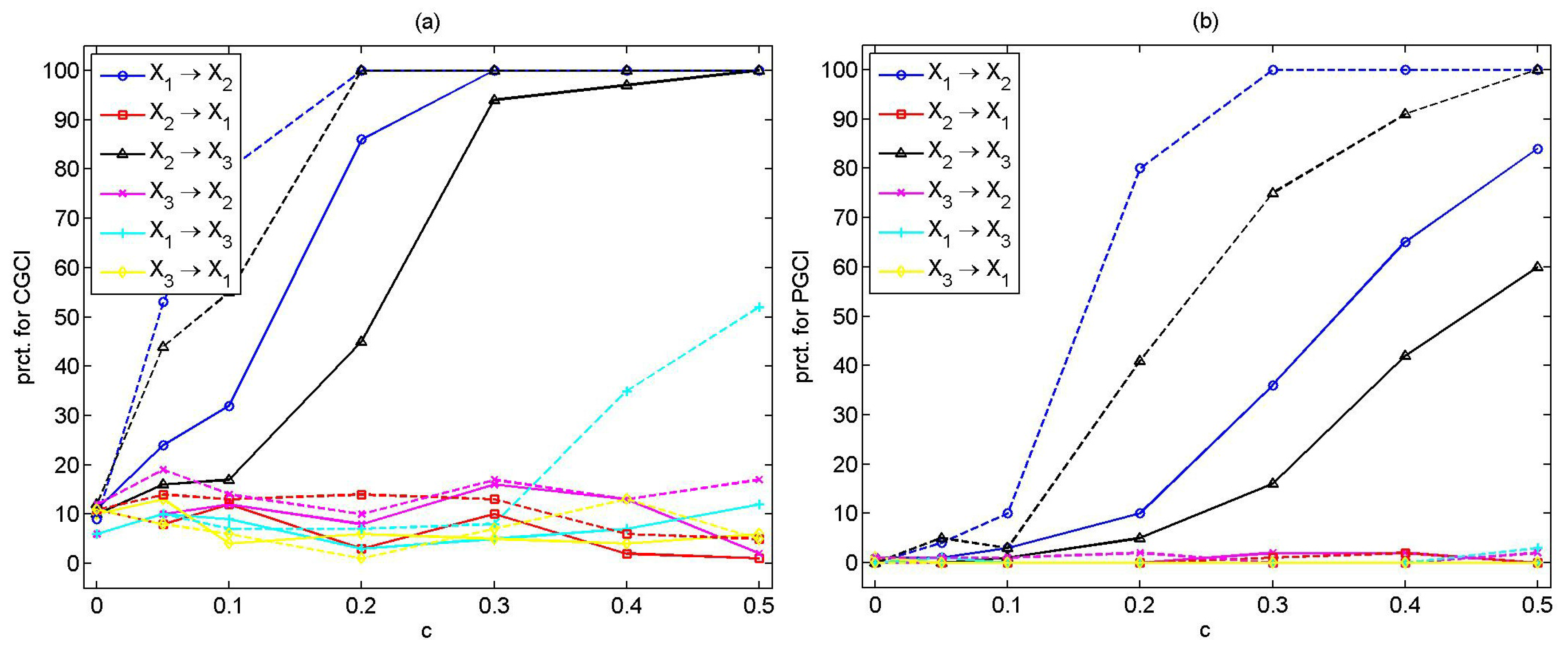
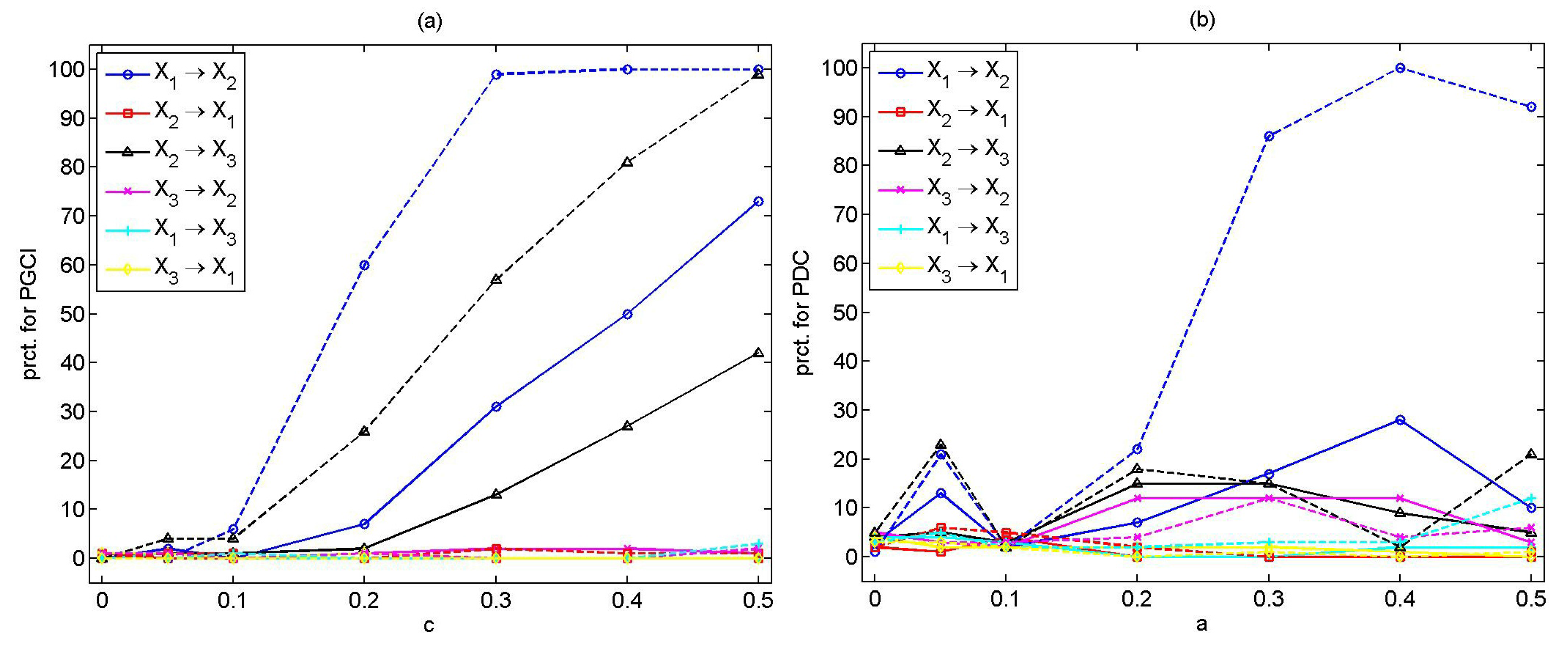
In order to evaluate the multivariate causality measures, the percentage of rejection of the null hypothesis of no causal effects ( H 0 ) in 100 realizations of the system is calculated for each possible pair of variables and for different time series lengths and free parameters of the measures. The focus when presenting the results is on the sensitivity of the measure or, respectively, the power of the significance test (the percentage of rejection at the significance level 5 % or α = 0 . 05 when there is true direct causality), as well as the specificity of the measure or size of the test (the percentage of rejection at α = 0 . 05 when there is no direct causality) and how these properties depend on the time series length and the measure-specific parameter.

4.1. Results for System 1

For the estimation of the linear measures, the order of the model, P, is set to one, as indicated from the Bayesian Information Criterion (BIC) and the Akaike Information Criterion (AIC), while for the estimation of PTE, m is also set to one. The PDC is estimated for the range of frequencies [ 0 , 0 . 5 ] , since the auto-spectra of the variables do not suggest a narrower range. Indeed, the p-values of PDC are all significant in [ 0 , 0 . 5 ] , when there is direct causality, and not significant, when there is no direct causality. The CGCI, PGCI, PDC and PTE correctly detect the direct causal effect for both time series lengths, n = 512 and 2048. All the aforementioned measures indicate 100 % rejection of H 0 for the true couplings, X 1 X 2 and X 2 X 3 , and low percentages for all other couplings. Their performance is not affected by the time series length, for the time series lengths considered. The estimated percentages are displayed for both n in Table 1.
The PSTE can only be estimated for m 2 , and therefore, results are obtained for m = 2 . The PSTE correctly detects the direct causalities for m = 2 ; however, it also indicates the indirect effect, X 1 X 3 , and the spurious causal effect, X 2 X 1 .
Only for this system, the PMIME with the threshold of A = 0 . 95 failed to detect the true direct effects, and the randomization test gave partial improvement (detection of one of the two true direct effects, X 2 X 3 ). This is merely a problem of using the fixed threshold, A = 0 . 95 , in this system, and following the adapted threshold proposed in [28], the two true direct effects could be detected for all realizations with n = 512 and n = 2048 with the largest rate of false rejection being 8 % .

4.2. Results for System 2

For the second simulation system, the model order is set to P = 5 , as indicated both by BIC and AIC. The embedding dimension, m, and L m a x 
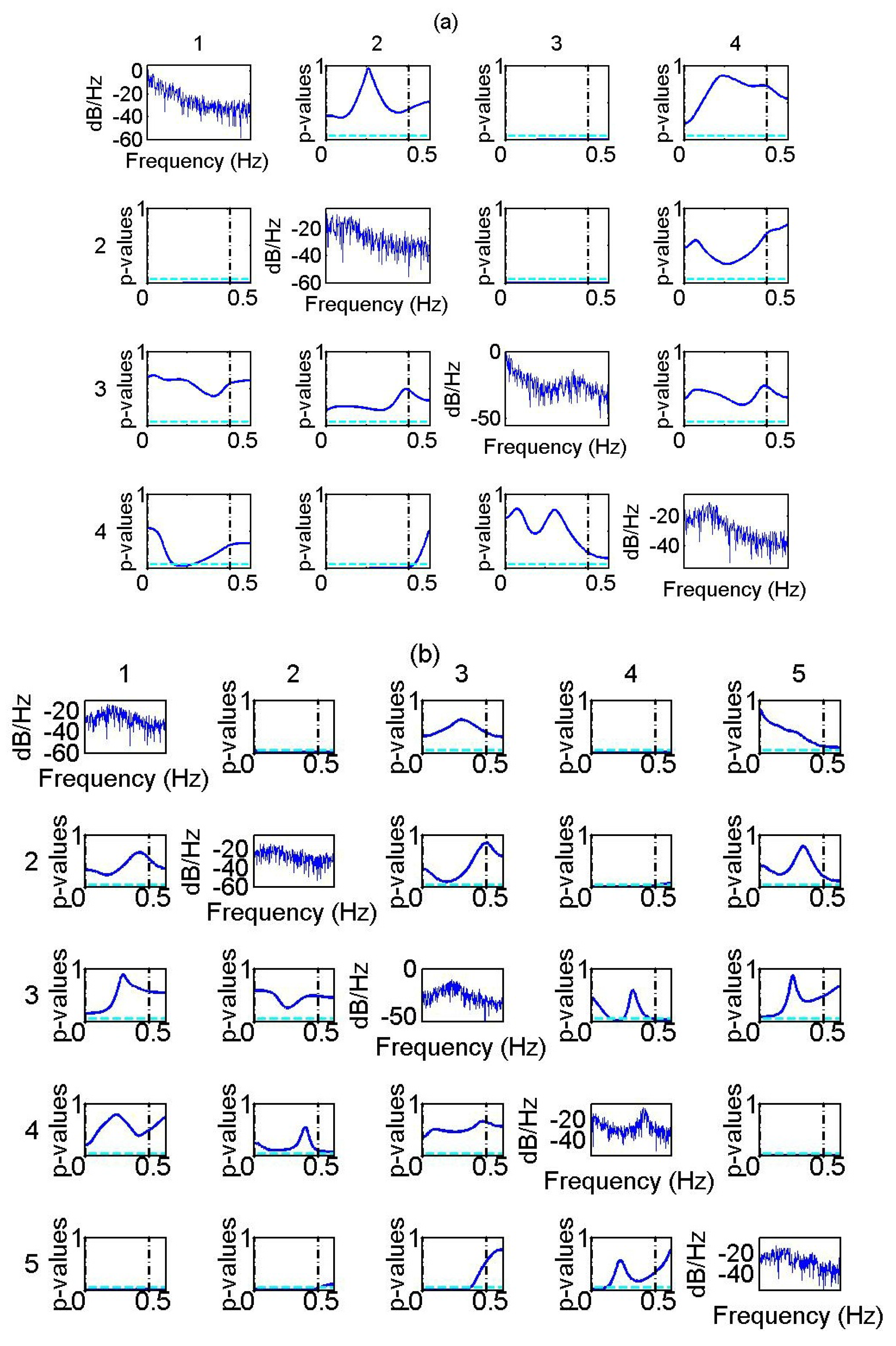
are also set to five. The PDC is estimated for the range of frequencies, [ 0 , 0 . 4 ] , since the auto-spectra of all the variables are higher in the range, [ 0 , 0 . 2 ] , while variable, X 3 , exhibits a peak in the range, [ 0 . 2 , 0 . 4 ] . Indicatively, the p-values from one realization of the system for the range of frequencies, [ 0 , 0 . 5 ] , is displayed in Figure 1a.
The CGCI, PGCI, PDC and PMIME correctly detect the direct couplings ( X 2 X 1 , X 1 X 3 , X 2 X 3 , X 4 X 2 ), as shown in Table 2. The performance of the CGCI and PDC is not affected by the time series length. The PGCI is also not affected by n, except for the causal effect, X 2 X 4 , where the PGCI falsely indicates causality for n = 2048 ( 20 % ). The PMIME indicates lower power of the test compared to the linear measures only for X 2 X 3 and n = 512 .
The PTE detects the direct causal relationships, apart from the coupling, X 2 X 3 , although the percentage of rejection in this direction increases with n (from 14 % for n = 512 to 39 % for n = 2048 ). Further, the erroneous relationships, X 1 X 4 ( 50 % ) and X 3 X 4 ( 29 % ), are observed for n = 2048 . Focusing on the PTE values, it can be observed that they are much higher for the directions of direct couplings than for the remaining directions. Moreover, the percentages of significant PTE values increase with n for the directions with direct couplings and decrease with n for all other couplings (see Table 3).
We note that the standard deviation of the estimated PTE values from the 100 realizations are low (on the order of 10 2 ). Thus, the result of having falsely statistically significant PTE values for X 1 X 4 and X 3 X 4 is likely due to insufficiency of the randomization test.
PSTE fails to detect the causal effects for the second coupled system for both time series lengths, giving rejections at a rate between 1 % and 24 % for all directions. The failure of PSTE may be due to the the high dimensionality of the rank vectors (the joint rank vector has dimension 21).

4.3. Results for System 3

The CGCI, PGCI, PDC, PTE and PMIME correctly detect all direct causal effects ( X 1 X 2 , X 1 X 4 , X 5 X 1 , X 2 X 4 , X 5 X 2 , X 5 X 3 , X 4 X 5 ) for P = m = L m a x = 4 (based on BIC and AIC), as shown in Table 4.
The PDC is again estimated in the range of frequencies, [ 0 , 0 . 4 ] , (see in Figure 1b the auto-spectra of the variables and the p-values from the parametric test of PDC from one realization of the system). The CGCI, PGCI and PDC perform similarly for the two time series lengths. The PTE indicates 100 % significant values for n = 2048 when direct causality exists. However, the PTE also indicates the spurious causality, X 5 X 4 , for n = 2048 ( 37 % ). The specificity of the PMIME is improved by the increase of n, and the percentage of positive PMIME values in case of no direct causal effects varies from 0 % to 22 % for n = 512 , while for n = 2048 , it varies from 0 % to 1 % . The PSTE again fails to detect the causal effects, giving very low percentage of rejection at all directions ( 2 % to 16 % ).
Since the linear causality measures CGCI, PGCI and PDC have been developed for the detection of direct causality in linear coupled systems, it was expected that these methods would be successfully applied to all linear systems. The nonlinear measures PMIME and PTE also seem to be able to capture the direct linear couplings in most cases, with PMIME following close the linear measures both in specificity and sensitivity.
In the following systems, we investigate the ability of the causality measures to correctly detect direct causal effects when nonlinearities are present.

4.4. Results for System 4

For the fourth coupled system, the BIC and AIC suggest to set P = 1 , 2 and 3. The performance of the linear measures does not seem to be affected by the choice of P. The PDC is estimated for frequencies in [ 0 . 1 , 0 . 4 ] . The auto-spectra of the three variables do not display any peaks or any upward/downward trends. No significant differences in the results are observed if a wider or narrower range of frequencies is considered. The linear measures, CGCI, PGCI and PDC, capture only the linear direct causal effect, X 2 X 3 , while they fail to detect the nonlinear relationships, X 1 X 2 and X 1 X 3 , for both time series lengths.
The PTE and the PMIME correctly detect all the direct couplings for the fourth coupled system for m = L m a x = 1 , 2 and 3. The percentage of significant values of the causality measures are displayed in Table 5. The PTE gives equivalent results for m = 1 and m = 2 . The PTE correctly detects the causalities for m = 3 , but at a smaller power of the significance test for n = 512 ( 63 % for X 1 X 2 , 46 % for X 2 X 3 and 43 % for X 1 X 3 ). The percentage of significant PMIME values is 100 % for the directions of direct couplings, and falls between 0 % and 6 % for all other couplings, and this holds for any L m a x = 1 , 2 or 3 and for both n.
The PSTE indicates the link X 2 X 3 for both time series lengths, while X 1 X 2 is detected only for n = 2048 . The PSTE fails to point out the causality, X 1 X 3 . The results for m = 2 and 3 are equivalent. In order to investigate whether the failure of PSTE to show X 1 X 3 is due to finite sample data, we estimate the PSTE also for n = 4096 . For m = 2 , it indicates the same results as for n = 2048 . For m = 3 , the PSTE detects all the direct causal effects, X 1 X 2 ( 99 % ), X 2 X 3 ( 100 % ), X 1 X 3 ( 86 % ), but X 3 X 1 ( 62 % ) is also erroneously detected.

4.5. Results for System 5

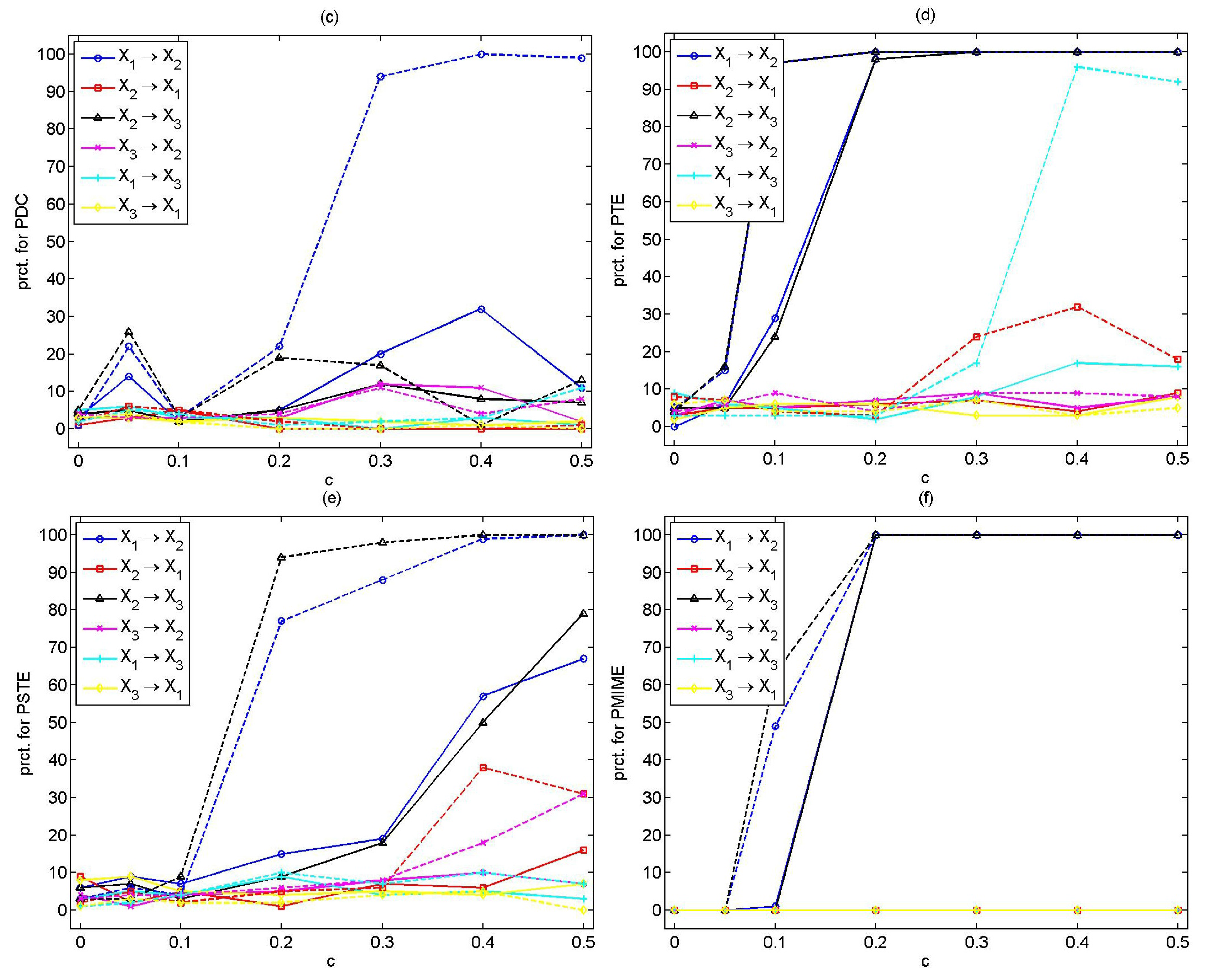
For the fifth coupled simulation system, we set the model order, P = 2 , based on the complexity of the system, and P = 3 , 4 and 5 using the AIC and BIC. The auto-spectra of the variables display peaks in [ 0 . 1 , 0 . 2 ] and [ 0 . 4 , 0 . 5 ] . The PDC is estimated for different ranges of frequencies to check its sensitivity with respect to the selection of the frequency range. When small frequencies are considered, the PDC seems to indicate larger percentages of spurious couplings; however, also, the percentages of significant PDC values at the directions of true causal effects are smaller. The results are presented for System 5 considering the range of frequencies, [ 0 . 4 , 0 . 5 ] .
The CGCI seems to be sensitive to the selection of the model order P, indicating some spurious couplings for the different P. The best performance for CGCI is achieved for P = 3 ; therefore, only results for P = 3 are shown. On the other hand, the PGCI turns out to be less dependent on P, giving similar results for P = 2 , 3, 4 and 5. The PTE is not substantially affected by the selection of the embedding dimension, m (at least for the examined coupling strengths); therefore, only results for m = 2 are discussed. The PSTE is sensitive to the selection of m, performing best for m = 2 and 3, while for m = 4 and 5, it indicates spurious and indirect causal effects. The PMIME does not seem to depend on L m a x . Results are displayed for L m a x = 5 
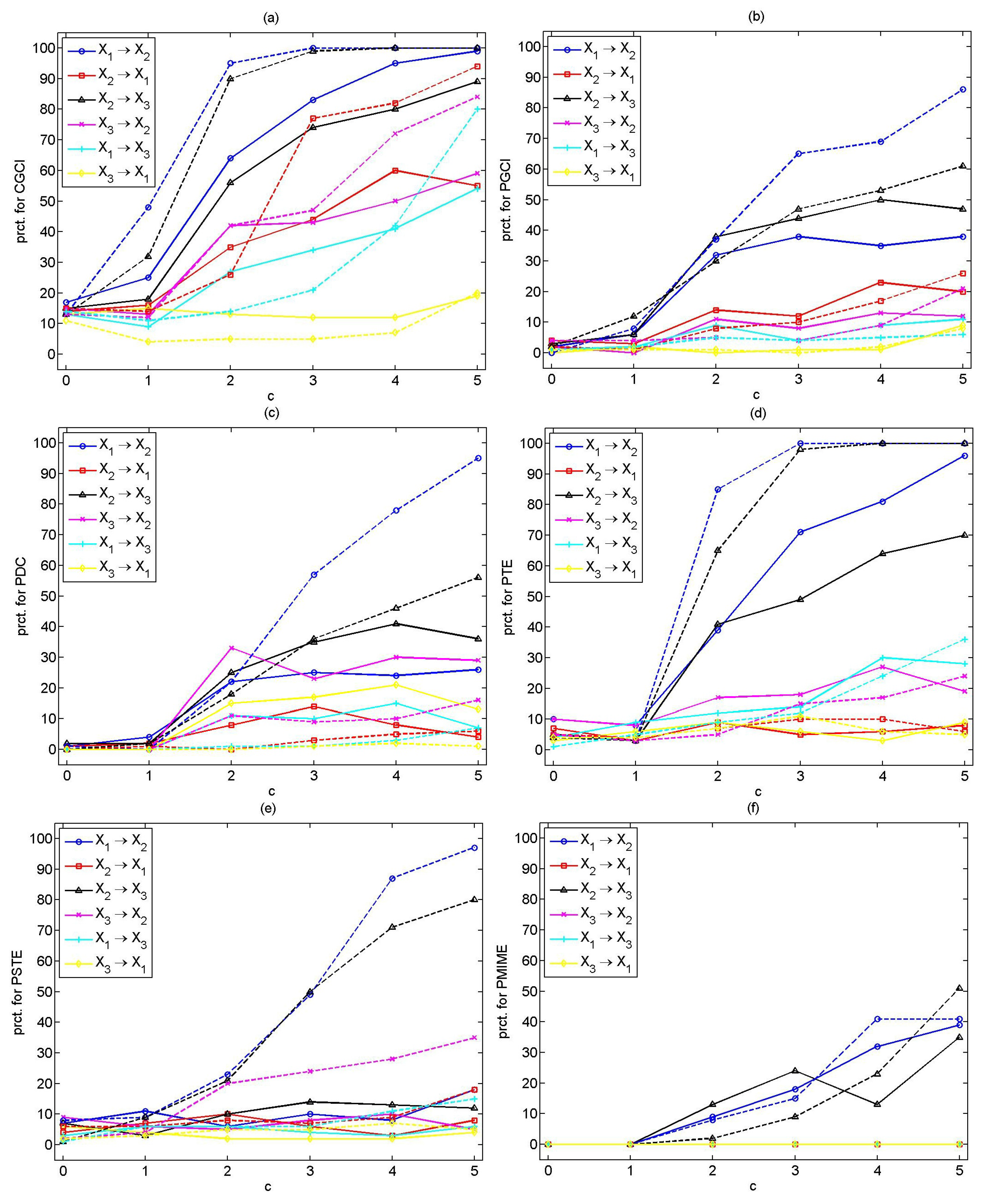
. The percentage of significant values for each measure are displayed in Figure 2, for all directions, for increasing coupling strength and for both n.
Most of the measures show good specificity, and the percentage of rejection for all pairs of the variables of the uncoupled system ( c = 0 ) is at the significance level, α = 0 . 05 , with only CGCI scoring a somehow larger percentage of rejection up to 17 % .
For the weak coupling strengths, c = 0 . 05 and 0.1, the causality measures cannot effectively detect the causal relationships or have a low sensitivity. The CGCI and the PTE seem to have the best performance, while the PMIME seems to be effective only for n = 2048 and c = 0 . 1 .
As the coupling strength increases, the sensitivity of the causality measures is improved. For c = 0 . 2 , the CGCI, PTE and PMIME correctly indicate the true couplings for both n, while the PGCI and the PSTE do this only for n = 2048 . The PDC has low power, even for n = 2048 . For c = 0 . 3 , nearly all measures correctly point out the direct causal effects (see Table 6). The best results are obtained with the PMIME, while the CGCI and PTE display similar performance. The PGCI and the PSTE are sensitive to the time series length and have a high power only for n = 2048 . The PDC performs poorly, giving low percentage of significant PDC values, even for n = 2048 . All measures have good specificity, with CGCI and PTE giving rejections well above the nominal level for some non-existing couplings.
Considering larger coupling strengths, the causality measures correctly indicate the true couplings, but also some spurious ones. The PMIME outperforms the other measures giving 100 % positive values for both n for X 1 X 2 and X 2 X 3 and 0 % at the remaining directions for c 0 . 2 . Indicative results for all measures are displayed for the strong coupling strength c = 0 . 5 in Table 7.
In order to investigate the effect of noise on each measure, we consider the coupled Hénon map (System 5) with the addition of Gaussian white noise with standard deviation 0 . 2 times the standard deviation of the original time series. Each measure is estimated again from 100 realizations from the noisy system for the same free parameters as considered in the noise-free case.
The CGCI is not significantly affected by the addition of noise, giving equivalent results for P = 3 as for the noise-free system. The CGCI detects the true causal effects even for weak coupling strength ( c 0 . 05 ). For different P values ( P = 2 , 4 or 5), some spurious and/or indirect causal effects are observed for c > 0 . 3 .
The PGCI is also not considerably affected by the addition of noise. The causal effects are detected only for coupling strengths, c 0 . 3 , for n = 512 , and for c 0 . 2 , for n = 2048 , while the power of the test increases with c and with n (see Figure 3a).
The PDC fails in the case of the noisy coupled Hénon maps, detecting only the coupling X 1 X 2 , for coupling strengths, c 0 . 2 and n = 2048 (see Figure 3b).
The PTE seems to be significantly affected by the addition of noise, falsely detecting the coupling, X 2 X 1 , X 3 X 2 , and the indirect coupling, X 1 X 3 , for strong coupling strengths. The performance of PTE is not significantly influenced by the choice of m. Indicative results are presented in Table 8 for m = 2 .
Noise addition does not seem to affect the performance of PSTE. Results for m = 2 are equivalent to the results obtained for the noise-free case. The power of the significance test increases with c and n. The PSTE is sensitive to the selection of m; as m increases, the percentage of significant PSTE values in the directions of no causal effects also increases.
The PMIME outperforms the other measures also for the noisy coupled Hénon maps, detecting the true couplings for c 0 . 2 for n = 512 ( 100 % ) and for c 0 . 1 for n = 2048 (for coupling strength c = 0 . 1 the percentages are 22 % and 23 % for X 1 X 2 , X 2 X 3 , respectively, and for c 0 . 2 , the percentages are 100 % , for both couplings).

4.6. Results for System 6

For System 6, we set P = 3 based on the complexity of the system and P = 5 regarding the AIC and BIC. The PTE, PSTE and PMIME are estimated for four different combinations of the free parameters, h and m ( L m a x for PMIME), i.e., for h = 1 and m = 3 , for h = 3 and m = 3 , for h = 1 and m = 5 and for h = 5 and m = 5 . The PDC is computed for the range of frequencies, [ 0 , 0 . 2 ] , based on the auto-spectra of the variables. As this system is a nonlinear flow, the detection of causal effects is more challenging compared to stochastic systems and nonlinear coupled maps. Indicative results for all causality measures are displayed for increasing coupling strengths in Figure 4.
The CGCI has poor performance, indicating many spurious causalities. The PGCI improves the specificity of the CGCI, but still, the percentages of statistically significant PGCI values increase with c for non-existing direct couplings (less for larger n). Similar results are obtained for P = 3 and 5. On the other hand, the PDC is sensitive to the selection of P, indicating spurious causal effects for all P. As P increases, the percentage of significant PDC values at the directions of no causal effects is reduced. However, the power of the test is also reduced.
The PTE is sensitive to the embedding dimension m and the number of steps ahead h, performing best for h = 1 and m = 5 . It fails to detect the causal effects for small c; however, for c > 1 , it effectively indicates the true couplings. The size of the test increases with c (up to 36 % for c = 5 and n = 2048 ), while the power of the test increases with n.
The PSTE is also affected by its free parameters, performing best for h = 3 and m = 3 . It is unable to detect the true causal effects for weak coupling strengths ( c 1 ) and for small time series lengths. The PSTE is effective only for c > 2 and n = 2048 . Spurious couplings are observed for strong coupling strengths c and n = 2048 .
The PMIME is also influenced by the choice of h and L m a x , indicating low sensitivity when setting h = 1 , but no spurious couplings, while for h = L m a x , the percentage of significant PMIME values for X 1 X 2 and X 2 X 3 is higher, but the indirect coupling X 1 X 3 is detected for strong coupling strengths. The PMIME has a poor performance for weak coupling strength ( c < 2 ).
As c increases, the percentages of significant values of almost all the causality measures increase, but not only at the true directions, X 1 X 2 and X 2 X 3 . Indicative results are presented in Table 9 for strongly coupled systems ( c = 5 ). The CGCI gives high percentages of rejection of H 0 for all couplings (very low specificity). This also holds for the PGCI, but at a lower significance level. The PTE correctly detects the two true direct causal effects for h = 1 and m = 5 , but at some significant degree, also the indirect coupling, X 1 X 3 , and the non-existing coupling, X 3 X 2 . The PSTE does not detect the direct couplings for n = 512 , but it does when n = 2048 ( 97 % for X 1 X 2 and 80 % for X 2 X 3 ), but then it detects also spurious couplings, most notably X 3 X 2 ( 35 % ). The PMIME points out only the direct causal effects, giving, however, a lower percentage than the other measures for h = 1 , L m a x = 5 . Its performance seems to be affected by the selection of h and L m a x . The nonlinear measures turn out to be more sensitive to their free parameters.

4.7. Results for System 7

For the last coupled simulation system, we set the model order P = 2 , 3, 4 based on AIC and BIC, while the PDC is estimated in the range of frequencies, [ 0 . 1 , 0 . 2 ] . The embedding dimension, m, for the estimation of PTE and PSTE, as well as L m a x for the estimation of PMIME, are set equal to P. Results for all causality measures are displayed in Table 10.
The CGCI (for P = 5 ) correctly indicates the causal effects for n = 512 , giving 100 % percentage of significant values at the direction X 1 X 2 and X 1 X 4 , but lower percentage at the directions X 1 X 3 ( 63 % ), X 4 X 5 ( 37 % ) and X 5 X 4 ( 42 % ). The power of the test increases with n, but spurious couplings are also detected for n = 2048 . For P = 2 , 3 and 4, the CGCI indicates more spurious couplings than for P = 5 .
System 7 favors the PGCI, as it has been specifically defined for systems with latent and exogenous variables. The PGCI denotes the couplings, X 1 X 2 , X 1 X 3 , X 1 X 4 and X 4 X 5 , even for n = 512 with a high percentage; however, it fails to detect the coupling, X 5 X 4 , for both n.
The PDC detects the true couplings at low percentage for n = 512 . The percentage increases with n = 2048 at the directions of the true couplings. However, there are also false indications of directed couplings.
The PTE does not seem to be effective in this setting for any of the considered m values, since it indicates many spurious causal effects, while it fails to detect X 4 X 5 . The PSTE completely fails in this case, suggesting significant couplings at all directions. The true causal effects are indicated by the PMIME, but here, as well, many spurious causal effects are also observed.

5. Discussion

In this paper, we have presented six multivariate causality measures that are able to detect the direct causal effects among simultaneously measured time series. The multivariate direct coupling measures are tested on simulated data from coupled and uncoupled systems of different complexity, linear and nonlinear, maps and flows. The linear causality measures and the PMIME can be used in complex systems with a large number of observed variables, but the PTE and the PSTE fail, because they involve estimation of probability distributions of high dimensional variables.
The simulation results suggest that for real world data, it is crucial to investigate the presence of nonlinearities and confirm the existence of causal effects by estimating more than one causality measure, sensitive to linear, as well as nonlinear causalities. Concerning the specificity of the coupling measures (in absence of direct causality), the PMIME outperforms the other measures, but for weak coupling, it is generally less sensitive than the PTE. In general, the PMIME indicated fewer spurious causal effects. Here, we considered only systems of a few variables, and for larger systems, the PMIME was found to outperform the PTE and, also, the CGCI [28].
Regarding the three first linear coupled systems in the simulation study, the CGCI, PGCI and PDC are superior to the nonlinear causality measures, both in sensitivity and specificity. The PMIME correctly indicates the coupling among the variables, but tends to have smaller sensitivity than the linear tests. The PTE cannot detect the true direct causality in all the examined linear systems and gives also some spurious results. The PSTE was the less effective one. For the last simulation system with the exogenous and latent variables (System 7), all but PGCI measures had low specificity, indicating only the true direct causal effects.
Concerning the nonlinear coupled system, the PTE and the PMIME outperform the other methods. The linear measures (CGCI, PGCI and PDC) fail to consistently detect the true direct causal effects (low sensitivity). The failure of the linear measures may not only be due to the fact that the system is nonlinear, but also due to the small time series lengths and the low model order. For example, the PDC correctly indicated the causal effects on simulated data from the coupled Rössler system for n = 50 , 000 and model order, P = 200 (see [49]). The PSTE requires large data sets to have a good power, while it gives spurious couplings at many cases. Though the PSTE performed overall worst in the simulation study, there are other settings in which it can be useful, e.g., in the presence of outliers or non-stationarity in mean, as slow drifts do not have a direct effect on the ranks. The addition of noise does not seem to affect the causality measures, CGCI, PGCI, PSTE and PMIME.
The free parameters were not optimized separately for each measure. For all systems, the parameters of model order, P, embedding dimension, m, and maximum lag, L m a x , were treated as one free parameter, the values of which were selected according to the complexity of each system and the standard criteria of AIC and BIC. The linear measures tend to be less sensitive to changes on this free parameter than the nonlinear ones. The PTE gave more consistent results than the PSTE for varying m, whereas the PMIME was not dependent on L m a x . For the nonlinear measures and the continuous-time system (three coupled Lorenz systems), we considered also the causalities at more than one step ahead, and the PTE, PSTE and PMIME were found to be sensitive to the selection of the steps ahead.
A point of concern regarding all direct causality measures, but the PMIME, is that the size of the significance test was high in many settings. This was observed for both types of spurious direct causal effect, i.e., when there is indirect coupling or when there is no causal effect. In many cases of non-existing direct causalities, although the observed test size was large, the estimated values of the measure were low compared to those in the presence of direct causalities. This raises also the question of the validity of the significance tests. The randomization test used time-shifted surrogates. Although it is simple and straightforward to implement, it may not always be sufficient, and further investigation for other randomization techniques is due for future work.
In conclusion, we considered six of the best-known measures of direct causality and studied their performance for different systems, time series lengths and free parameters. The worst performance was observed for the PSTE, since it completely failed in the case of the linear coupled systems, while for nonlinear systems, it required large data sets. The other measures scored differently in terms of sensitivity and specificity in the different settings. The CGCI, PGCI and PDC outperformed the nonlinear ones in the case of the linear coupled simulation systems, while in the presence of exogenous and latent variables, the PGCI seems to be the most effective one. The PMIME seems to have the best performance for nonlinear and noisy systems, while always obtaining the highest specificity, indicating no spurious effects. It is the intention of the authors to pursue the comparative study on selected real applications.

Acknowledgements

The research project is implemented within the framework of the Action “Supporting Postdoctoral Researchers” of the Operational Program, “Education and Lifelong Learning” (Action’s Beneficiary: General Secretariat for Research and Technology), and is co-financed by the European Social Fund (ESF) and the Greek State.

Conflict of Interest

The authors declare no conflict of interest.

References

  1. Granger, C.W.J. Investigating causal relations by econometric models and cross-spectral methods. Econometrica 1969, 37, 424–438. [Google Scholar] [CrossRef]
  2. Geweke, J. Measurement of linear dependence and feedback between multiple time series. J. Am. Stat. Assoc. 1982, 77, 304–313. [Google Scholar] [CrossRef]
  3. Baek, E.; Brock, W. A general test for nonlinear Granger causality: Bivariate model, 1992. Working paper. University of Wisconsin: Madison, WI, USA.
  4. Hiemstra, C.; Jones, J.D. Testing for linear and nonlinear Granger causality in the stock Price-Volume Relation. J. Financ. 1994, 49, 1639–1664. [Google Scholar] [CrossRef]
  5. Aparicio, F.; Escribano, A. Information-theoretic analysis of serial correlation and cointegration. Stud. Nonlinear Dyn. Econom. 1998, 3, 119–140. [Google Scholar]
  6. Freiwald, V.A.; Valdes, P.; Bosch, J.; Biscay, R.; Jimenez, J.; Rodriguez, L. Testing non-linearity and directedness of interactions between neural groups in the macaque inferotemporal cortex. J. Neurosci. Methods 1999, 94, 105–119. [Google Scholar] [CrossRef]
  7. Marinazzo, D.; Pellicoro, M.; Stramaglia, S. Kernel method for nonlinear Granger causality. Phys. Rev. Lett. 2008, 100, 144103. [Google Scholar] [CrossRef] [PubMed]
  8. Arnhold, J.; Grassberger, P.; Lehnertz, K.; Elger, C.E. A robust method for detecting interdependences: Application to intracranially recorded EEG. Physica D: Nolinear Phenom. 1999, 134, 419–430. [Google Scholar] [CrossRef]
  9. Romano, M.; Thiel, M.; Kurths, J.; Grebogi, C. Estimation of the direction of the coupling by conditional probabilities of recurrence. Phys. Rev. E 2007, 76, 036211. [Google Scholar] [CrossRef] [PubMed]
  10. Marko, H. The bidirectional communication theory-a generalization of information theory. IEEE Trans. Commun. 1973, 21, 1345–1351. [Google Scholar] [CrossRef]
  11. Schreiber, T. Measuring information transfer. Phys. Rev. Lett. 2000, 85, 461–464. [Google Scholar] [CrossRef] [PubMed]
  12. Paluš, M. Coarse-grained entropy rates for characterization of complex time series. Physica D: Nolinear Phenom. 1996, 93, 64–77. [Google Scholar] [CrossRef]
  13. Rosenblum, M.G.; Pikovsky, A.S. Detecting direction of coupling in interacting oscillators. Phys. Rev. E 2001, 64, 045202. [Google Scholar] [CrossRef] [PubMed]
  14. Nolte, G.; Ziehe, A.; Nikulin, V.; Schlogl, A.; Kramer, N.; Brismar, T.; Muller, K.R. Robustly estimating the flow direction of information in complex physical systems. Phys. Rev. Lett. 2008, 100, 234101. [Google Scholar] [CrossRef] [PubMed]
  15. Blinowska, K.J.; Kus, R.; Kaminski, M. Granger causality and information flow in multivariate processes. Phys. Rev. E 2004, 70, 050902. [Google Scholar] [CrossRef] [PubMed]
  16. Kus, R.; Kaminski, M.; Blinowska, K.J. Determination of EEG activity propagation: Pair-wise versus multichannel estimate. IEEE Trans. Biomed. Eng. 2004, 51, 1501–1510. [Google Scholar] [CrossRef] [PubMed]
  17. Eichler, M. Graphical modelling of multivariate time series. Probab. Theory Relat. Fields 2012, 153, 233–268. [Google Scholar] [CrossRef]
  18. Guo, S.; Seth, A.K.; Kendrick, K.M.; Zhou, C.; Feng, J. Partial granger causality–eliminating exogenous inputs and latent variables. J. Neurosci. Methods 2008, 172, 79–93. [Google Scholar] [CrossRef] [PubMed]
  19. Kaminski, M.J.; Blinowska, K.J. A new method of the description of the information flow in the brain structures. Biol. Cybern. 1991, 65, 203–210. [Google Scholar] [CrossRef] [PubMed]
  20. Baccala, L.A.; Sameshima, K. Partial directed coherence: A new concept in neural structure determination. Biol. Cybern. 2001, 84, 463–474. [Google Scholar] [CrossRef] [PubMed]
  21. Korzeniewska, A.; Manczak, M.; Kaminski, M.; Blinowska, K.; Kasicki, S. Determination of information flow direction between brain structures by a modified directed transfer function (dDTF) method. J. Neurosci. Methods 2003, 125, 195–207. [Google Scholar] [CrossRef]
  22. Chavez, M.; Martinerie, J.; Quyen, M. Statistical assessment of non-linear causality: Application to epileptic EEG signals. J. Neurosci. Methods 2003, 124, 113–128. [Google Scholar] [CrossRef]
  23. Verdes, P. Assessing causality from multivariate time series. Phys. Rev. E 2005, 72, 026222. [Google Scholar] [CrossRef] [PubMed]
  24. Vakorin, V.A.; Krakovska, O.A.; McIntosh, A.R. Confounding effects of indirect connections on causality estimation. J. Neurosci. Methods 2009, 184, 152–160. [Google Scholar] [CrossRef] [PubMed]
  25. Papana, A.; Kugiumtzis, D.; Larsson, P.G. Detection of direct causal effects and application in the analysis of electroencephalograms from patients with epilepsy. Int. J. Bifurc. Chaos 2012, 22. [Google Scholar] [CrossRef]
  26. Vlachos, I.; Kugiumtzis, D. Non-uniform state space reconstruction and coupling detection. Phys. Rev. E 2010, 82, 016207. [Google Scholar] [CrossRef] [PubMed]
  27. Faes, L.; Nollo, G.; Porta, A. Information-based detection of nonlinear Granger causality in multivariate processes via a nonuniform embedding technique. Phys. Rev. E 2011, 83, 051112. [Google Scholar] [CrossRef] [PubMed]
  28. Kugiumtzis, D. Direct coupling information measure from non-uniform embedding. Phys. Rev. E 2013, 87, 062918. [Google Scholar] [CrossRef] [PubMed]
  29. Jizba, P.; Kleinert, H.; Shefaat, M. Rényi’s information transfer between financial time series. Physica A: Stat. Mech. Appl. 2012, 391, 2971–2989. [Google Scholar] [CrossRef]
  30. Staniek, M.; Lehnertz, K. Symbolic transfer entropy. Phys. Rev. Lett. 2008, 100, 158101. [Google Scholar] [CrossRef] [PubMed]
  31. Kugiumtzis, D. Transfer entropy on rank vectors. J. Nonlinear Syst. Appl. 2012, 3, 73–81. [Google Scholar]
  32. Kugiumtzis, D. Partial transfer entropy on rank vectors. Eur. Phys. J. Spec. Top. 2013, 222, 401–420. [Google Scholar] [CrossRef]
  33. Smirnov, D.A.; Andrzejak, R.G. Detection of weak directional coupling: Phase-dynamics approach versus state-space approach. Phys. Rev. E 2005, 71, 036207. [Google Scholar] [CrossRef] [PubMed]
  34. Faes, L.; Porta, A.; Nollo, G. Mutual nonlinear prediction as a tool to evaluate coupling strength and directionality in bivariate time series: Comparison among different strategies based on k nearest neighbors. Phys. Rev. E 2004, 78, 026201. [Google Scholar] [CrossRef] [PubMed]
  35. Papana, A.; Kugiumtzis, D.; Larsson, P.G. Reducing the bias of causality measures. Phys. Rev. E 2011, 83, 036207. [Google Scholar] [CrossRef] [PubMed]
  36. Silfverhuth, M.J.; Hintsala, H.; Kortelainen, J.; Seppanen, T. Experimental comparison of connectivity measures with simulated EEG signals. Med. Biol. Eng. Comput. 2012, 50, 683–688. [Google Scholar] [CrossRef] [PubMed]
  37. Dufour, J.M.; Taamouti, A. Short and long run causality measures: Theory and inference. J. Econ. 2010, 154, 42–58. [Google Scholar] [CrossRef]
  38. Florin, E.; Gross, J.; Pfeifer, J.; Fink, G.; Timmermann, L. Reliability of multivariate causality measures for neural data. J. Neurosci. Methods 2011, 198, 344–358. [Google Scholar] [CrossRef] [PubMed]
  39. Wu, M.-H.; Frye, R.E.; Zouridakis, G. A comparison of multivariate causality based measures of effective connectivity. Comput. Biol. Med. 2011, 21, 1132–1141. [Google Scholar] [CrossRef] [PubMed]
  40. Blinowska, K.J. Review of the methods of determination of directed connectivity from multichannel data. Med. Biol. Eng. Comput. 2011, 49, 521–529. [Google Scholar] [CrossRef] [PubMed]
  41. Brandt, P.T.; Williams, J.T. Multiple Time Series Models; Sage Publications, Inc.: Thousand Oaks, CA, USA, 2007; chapter 2; pp. 32–34. [Google Scholar]
  42. Benjamini, Y.; Hochberg, Y. Controlling the false discovery rate: A practical and powerful approach to multiple testing. J. R. Stat. Soc. Ser. B 1995, 57, 289–300. [Google Scholar]
  43. Akaike, H. A new look at the statistical model identification. IEEE Trans. Autom. Control 1974, 19, 716–723. [Google Scholar] [CrossRef]
  44. Schwartz, G. Estimating the dimension of a model. Ann. Stat. 1978, 5, 461–464. [Google Scholar] [CrossRef]
  45. Ding, M.; Chen, Y.; Bressler, S.L. Granger Causality: Basic Theory and Applications to Neuroscience. In Handbook of Time Series Analysis: Recent Theoretical Developments and Applications; Schelter, B., Winterhalder, M., Timmer, J., Eds.; Wiley-VCH Verlag: Berlin, Germany, 2006; chapter 17; pp. 437–460. [Google Scholar]
  46. Schelter, B.; Winterhalder, M.; Eichler, M.; Peifer, M.; Hellwig, B.; Guschlbauer, B.; Lucking, C.H.; Dahlhaus, R.; Timmer, J. Testing for directed influences in neuroscience using partial directed coherence. J. Neurosci. Methods 2006, 152, 210–219. [Google Scholar] [CrossRef] [PubMed]
  47. Takahashi, D.Y.; Baccala, L.A.; Sameshima, K. Connectivity inference between neural structures via partial directed coherence. J. Appl. Stat. 2007, 34, 1255–1269. [Google Scholar]
  48. Kraskov, A.; Stögbauer, H.; Grassberger, P. Estimating mutual information. Phys. Rev. E 2004, 69, 066138. [Google Scholar] [CrossRef] [PubMed]
  49. Winterhalder, M.; Schelter, B.; Hesse, W.; Schwab, K.; Leistritz, L.; Klan, D.; Bauer, R.; Timmer, J.; Witte, H. Comparison of linear signal processing techniques to infer directed interactions in multivariate neural systems. Signal Process. 2005, 85, 2137–2160. [Google Scholar] [CrossRef]
  50. Gourévitch, B.; Le Bouquin-Jeannés, R.; Faucon, G. Linear and nonlinear causality between signals: methods, examples and neurophysiological applications. Biol. Cybern. 2006, 95, 349–369. [Google Scholar] [CrossRef] [PubMed]
  51. Stefanski, A. Determining Thresholds of Complete Synchronization, and Application; World Scientific: Singapore, Singapore, 2009. [Google Scholar]
  52. Wilke, C.; van Drongelen, W.; Kohrman, M.; Hea, B. Identification of epileptogenic foci from causal analysis of ECoG interictal spike activity. Clin. Neurophys. 2009, 120, 1449–1456. [Google Scholar] [CrossRef] [PubMed]
  53. Efron, B.; Tibshirani, R. An Introduction to the Bootstrap; Chapman and Hall: New York, NY, USA, 1994. [Google Scholar]
  54. Faes, L.; Porta, A.; Nollo, G. Testing frequency-domain causality in multivariate time series. IEEE Trans. Biomed. Eng. 2010, 57, 1897–1906. [Google Scholar] [CrossRef] [PubMed]
  55. Quian Quiroga, R.; Kraskov, A.; Kreuz, T.; Grassberger, P. Performance of different synchronization measures in real data: A case study on electroencephalographic signals. Phys. Rev. E 2002, 65, 041903. [Google Scholar] [CrossRef] [PubMed]
  56. Yu, G.H.; Huang, C.C. A distribution free plotting position. Stoch. Environ. Res. Risk Assess. 2001, 15, 462–476. [Google Scholar] [CrossRef]
  57. Seth, A.K. A MATLAB toolbox for Granger causal connectivity analysis. J. Neurosci. Methods 2010, 186, 262–273. [Google Scholar] [CrossRef] [PubMed]
Figure 1. Graph summarizing the causal influences for one realization of System 2 (rows → columns) in (a) and System 3 in (b). The p-values from the partial directed coherence (PDC) are displayed for the range of frequencies, [ 0 , 0 . 5 ] , while the dotted vertical lines indicate the frequency, 0.4. The horizontal cyan lines indicate the 5 % -significance level. The auto-spectra are shown on the diagonal.
Entropy 15 02635 g001
Figure 2. Percentage of significant (a) CGCI ( P = 3 ); (b) PGCI ( P = 3 ); (c) PDC ( P = 3 ); (d) PTE ( m = 2 ); (e) PSTE ( m = 2 ); and (f) PMIME ( L m a x = 5 ) values, for System 5, for increasing coupling strengths, c, at all directions and for both n (for n = 512 , solid lines, for n = 2048 , dotted lines).
Entropy 15 02635 g002aEntropy 15 02635 g002b
Figure 3. Percentage of significant (a) PGCI ( P = 3 ) and (b) PDC ( P = 3 ) values, for System 5 with addition of noise (solid lines for n = 512 , dotted lines for for n = 2048 ).
Entropy 15 02635 g003
Figure 4. Percentage of significant (a) CGCI ( P = 5 ); (b) PGCI ( P = 5 ); (c) PDC ( P = 5 ); (d) PTE ( h = 1 , m = 5 ); (e) PSTE ( h = 3 , m = 3 ); and (f) PMIME ( h = 1 , L m a x = 5 ) values, for System 6, for increasing coupling strengths, c, at all directions and for both n (solid lines for n = 512 , dotted lines for n = 2048 ).
Entropy 15 02635 g004
Table 1. Percentage of statistically significant values of the causality measures for System 1, P = m = L m a x = 1 [ m = 2 for partial symbolic transfer entropy (PSTE)]. The directions of direct causal effects are pointed out in bold. When the same percentage has been found for both n, a single number is displayed in the cell.
n = 512 /2048CGCIPGCIPDCPTEPSTEPMIME
X 1 X 2 1001001001001001 / 0
X 2 X 1 4 / 32 / 12 / 38 / 558 / 1002 / 7
X 2 X 3 100100100100100100
X 3 X 2 7 / 68 / 133 / 57 / 250
X 1 X 3 3 / 50 / 22 / 35 / 793 / 1000
X 3 X 1 2 / 7033 / 214 / 437 / 7
Table 2. Percentage of statistically significant values of the causality measures for System 2, P = m = L m a x = 5 . The directions of direct causal effects are displayed in bold face. CGCI, conditional Granger causality index; PGCI, partial Granger causality index; PDC, partial directed coherence; PTE, partial transfer entropy; PSTE, partial symbolic transfer entropy; PMIME, partial mutual information on mixed embedding.
n = 512 /2048CGCIPGCIPDCPTEPSTEPMIME
X 1 X 2 6 / 2106 / 117 / 200
X 2 X 1 1001001001005 / 11100
X 1 X 3 1001001001007 / 15100
X 3 X 1 5 / 3006 / 146 / 90
X 1 X 4 6 / 7007 / 502 / 243 / 0
X 4 X 1 3 / 2002 / 550
X 2 X 3 10098 / 10094 / 10014 / 399 / 1864 / 99
X 3 X 2 8 / 5004 / 165 / 31 / 0
X 2 X 4 7 / 63 / 2005 / 81 / 202 / 0
X 4 X 2 1001001001007 / 2100
X 3 X 4 4 / 30 / 208 / 292 / 83 / 0
X 4 X 3 4 / 50075 / 60
Table 3. Mean PTE values from 100 realizations of System 2, for P = 5 and n = 512 , 2048. The values of the true direct couplings are highlighted.
mean X 1 X 2 X 2 X 1 X 1 X 3 X 3 X 1 X 1 X 4 X 4 X 1
n = 512 0.00420.09200.07720.00340.00670.0043
n = 2048 0.00290.12210.09650.00160.00340.0020
X 2 X 3 X 3 X 2 X 2 X 4 X 4 X 2 X 3 X 4 X 4 X 3
n = 512 0.00600.00520.00950.09980.00710.0033
n = 2048 0.00590.00320.00610.13550.00420.0013
Table 4. Percentages of statistically significant values of causality measures for System 3, for P = m = L m a x = 4 .
n = 512 /2048CGCIPGCIPDCPTEPSTEPMIME
X 1 X 2 10086 / 10092 / 10081 / 1008 / 7100
X 2 X 1 7 / 32 / 007 / 23 / 818 / 0
X 1 X 3 6 / 52 / 003 / 44 / 102 / 0
X 3 X 1 1 / 2005 / 42 / 414 / 0
X 1 X 4 10010010052 / 1002 / 9100
X 4 X 1 7 / 41 / 006 / 44 / 1012 / 0
X 1 X 5 5206 / 107 / 1216 / 0
X 5 X 1 10098 / 10099 / 1001002 / 16100
X 2 X 3 42 / 004 / 69 / 52 / 0
X 3 X 2 6 / 21 / 004 / 25 / 49 / 1
X 2 X 4 10099 / 10096 / 10018 / 77794 / 100
X 4 X 2 5 / 9005 / 42 / 49 / 0
X 2 X 5 6 / 42 / 305 / 44 / 622 / 0
X 5 X 2 10096 / 10099 / 10099 / 1003 / 8100
X 3 X 4 3 / 71 / 003 / 45 / 80
X 4 X 3 41 / 003 / 64 / 54 / 0
X 3 X 5 4 / 3107 / 4614 / 0
X 5 X 3 10087 / 10084 / 10049 / 973 / 15100
X 4 X 5 1001001001006 / 4100
X 5 X 4 5 / 20017 / 376 / 141 / 0
Table 5. Percentage of statistically significant values of the causality measures for System 4, P = m = L m a x = 2 .
n = 512 /2048CGCIPGCIPDCPTEPSTEPMIME
X 1 X 2 12 / 71297 / 10010 / 69100
X 2 X 1 2 / 70 / 11 / 08 / 94 / 83 / 0
X 2 X 3 10073 / 10010076 / 10069 / 100100
X 3 X 2 7 / 43 / 1143 / 94 / 0
X 1 X 3 71 / 00 / 186 / 1001 / 7100
X 3 X 1 4 / 5004 / 68 / 210
Table 6. Percentage of statistically significant values of the causality measures for System 5 for c = 0 . 3 , where P = 3 , m = 2 and L m a x = 5 .
n = 512 /2048CGCIPGCIPDCPTEPSTEPMIME
X 1 X 2 10036 / 10020 / 9410019 / 88100
X 2 X 1 10 / 130 / 10 / 27 / 247 / 60
X 2 X 3 94 / 10016 / 7512 / 1910018 / 98100
X 3 X 2 16 / 172 / 012 / 4980
X 1 X 3 5 / 800 / 18 / 174 / 70
X 3 X 1 5 / 702 / 03 / 75 / 40
Table 7. Percentages of statistically significant values of the causality measures for System 5 for c = 0 . 5 , where P = 3 , m = 2 and L m a x = 5 .
n = 512 /2048CGCIPGCIPDCPTEPSTEPMIME
X 1 X 2 10084 / 10011 / 9910067 / 100100
X 2 X 1 1 / 500 / 19 / 1816 / 310
X 2 X 3 10060 / 1007 / 1310079 / 100100
X 3 X 2 2 / 170 / 22 / 887 / 310
X 1 X 3 12 / 520 / 31 / 1116 / 923 / 70
X 3 X 1 6 / 502 / 08 / 57 / 00
Table 8. Percentages of statistically significant PTE ( m = 2 ) values for System 5 with the addition of noise.
n = 512 /2048 X 1 X 2 X 2 X 1 X 2 X 3 X 3 X 2 X 1 X 3 X 3 X 1
c = 0 2 / 55 / 645 / 710 / 17 / 6
c = 0 . 05 6 / 1735 / 204 / 53 / 67 / 1
c = 0 . 1 22 / 986 / 222 / 983 / 74 / 55 / 8
c = 0 . 2 1006 / 1199 / 1004 / 71 / 54 / 2
c = 0 . 3 10010 / 521008 / 2212 / 274 / 8
c = 0 . 4 1009 / 791006 / 5024 / 977 / 10
c = 0 . 5 10023 / 951007 / 4839 / 1008 / 13
Table 9. Percentage of statistically significant values of the causality measures for System 6 with c = 5 , where P = 5 , h = 1 and m = 5 for PTE, h = 3 and m = 3 for PSTE and h = 1 and L m a x = 5 for PMIME.
n = 512 /2048CGCIPGCIPDCPTEPSTEPMIME
X 1 X 2 99 / 10038 / 8626 / 9596 / 10018 / 9739 / 41
X 2 X 1 55 / 9420 / 264 / 68 / 68 / 180
X 2 X 3 89 / 10047 / 6136 / 5670 / 10012 / 8035 / 51
X 3 X 2 59 / 8412 / 2129 / 1619 / 245 / 350
X 1 X 3 54 / 8011 / 67 / 728 / 366 / 150
X 3 X 1 19 / 209 / 813 / 19 / 54 / 50
Table 10. Percentage of statistically significant values of the causality measures for System 7, where P = m = L m a x = 3 .
n = 512 /2048CGCIPGCIPDCPTEPSTEPMIME
X 1 X 2 10010047 / 10010047 / 31100
X 2 X 1 8 / 2607 / 236 / 986 / 1000
X 1 X 3 63 / 10010057 / 10036 / 91100100
X 3 X 1 6 / 81 / 81 / 298 / 10032 / 26100
X 1 X 4 10010073 / 10010031 / 84100
X 4 X 1 602 / 054 / 9673 / 10087 / 23
X 1 X 5 13 / 753 / 82 / 110 / 110020 / 9
X 5 X 1 9 / 501 / 25 / 161001 / 0
X 2 X 3 14 / 3607 / 3049 / 7540 / 243 / 41
X 3 X 2 9 / 1204 / 340 / 661001 / 0
X 2 X 4 11 / 383 / 07 / 2936 / 8191 / 920
X 4 X 2 7 / 1018 / 222 / 10 / 21000
X 2 X 5 10 / 3705 / 2947 / 6910086 / 94
X 5 X 2 5 / 701 / 320 / 4972 / 961 / 0
X 3 X 4 1205 / 388 / 1001000
X 4 X 3 5 / 1002 / 214 / 5998 / 10015 / 0
X 3 X 5 8 / 1304 / 11 / 21000
X 5 X 3 7 / 1101 / 314 / 431005 / 0
X 4 X 5 37 / 9483 / 10023 / 886 / 794 / 100100
X 5 X 4 42 / 1006 / 420 / 7610078 / 75100

