Linearized Transfer Entropy for Continuous Second Order Systems

Abstract

The transfer entropy has proven a useful measure of coupling among components of a dynamical system. This measure effectively captures the influence of one system component on the transition probabilities (dynamics) of another. The original motivation for the measure was to quantify such relationships among signals collected from a nonlinear system. However, we have found the transfer entropy to also be a useful concept in describing linear coupling among system components. In this work we derive the analytical transfer entropy for the response of coupled, second order linear systems driven with a Gaussian random process. The resulting expression is a function of the auto- and cross-correlation functions associated with the system response for different degrees-of-freedom. We show clearly that the interpretation of the transfer entropy as a measure of “information flow” is not always valid. In fact, in certain instances the “flow” can appear to switch directions simply by altering the degree of linear coupling. A safer way to view the transfer entropy is as a measure of the ability of a given system component to predict the dynamics of another.

1. Introduction

One of the biggest challenges in the modeling and analysis of dynamical systems is understanding coupling mechanisms among different system components. Whether one is studying coupling on a small scale (e.g., neurons in a biological system) or large scale (e.g. coupling among widely separated geographical locations due to climate), understanding the functional form, strength, and/or direction of the coupling between two or more system components is a non-trivial task. However, this understanding is necessary if we are to build accurate models of the coupled system and make predictions (our ultimate goal). Accurately assessing the functional form of the coupling is beyond the scope of this work. To do so would require positing various models for a particular coupled system and then testing the predictive power of those models against observed data. Rather, the focus here is on understanding the strength and direction of the coupling among two system components. This task can be accomplished by forming a general hypothesis about what it means for two system components to be coupled, and then testing that hypothesis against observation. It is in this framework that the transfer entropy is operates.

The transfer entropy (TE) is a scalar measure designed to capture both the magnitude and direction of coupling among two components of a dynamical system. This measure was posed initially for data described by discrete probability distributions [1] and was later extended to continuous random variables [2]. By construction, this measure quantifies a general definition of coupling that is appropriate for both linear and nonlinear systems. Moreover, TE is defined in such a way as to provide insight into the direction of the coupling (is component A driving component B or vice-versa?). Since its introduction, the TE has been applied to a diverse set of systems, including biological [1,3], chemical [4], economic [5], structural [6,7], and climate [8]. A number of papers in the Neurosciences also have focused on the TE as a useful way to draw inference about coupling [9,10,11]. In each case the TE provided information about the system that traditional linear measures of coupling (e.g., cross-correlation) could not.

The TE has also been linked to other concepts of coupling such as “Wiener-Granger Causality”. in fact, for the class of systems studied in this work the TE can be shown to be entirely equivalent to measures of Granger causality [12]. Linkages to other models and concepts of dynamical coupling such as conditional mutual information [13] and Dynamic Causal Modeling (DCM) [14], are also possible for certain special cases. The connectivity model assumed by DCM is fundamentally nonlinear (specifically bilinear), however as the degree of nonlinearity decreases the form of the DCM model approaches that of the model studied here.

Although the TE was designed as a way to gain insight into nonlinear system coupling, we have found the TE to be quite useful in the study of linear systems as well. In this special case, analytical expressions for the TE are possible and can be used to provide useful insight into the behavior of the TE. Furthermore, unlike in the general case, the linearized TE can be easily estimated from observed data. This work is therefore devoted to the understanding of TE as applied to coupled, driven linear systems. Specifically, we consider coupling among components of a general, second order linear structural system driven by a Gaussian random process. The particular model studied is used to describe numerous phenomena, including structural dynamics, electrical circuits, heat transfer, etc. [15]. As such, it presents an opportunity to better understand the properties of the TE for a broad class of dynamical systems. Section 1 develops the general analytical expression for the TE in terms of the covariance matrices associated with different combinations of system response data. Section 2 specifies the general model under study and derives the TE for the model response data. Section 3 and Section 4 present results and concluding remarks.

2. Mathematical Development

In what follows we assume that we have observed the signals $x_i\left(t_n\right),i=1\cdots M$ as the output of a dynamical system and that we have sampled these signals at times $t_n,n=1\cdots N$. The system is assumed to be appropriately modeled as a mixture of deterministic and stochastic components, hence we choose to model each sampled value $x_i\left(t_n\right)$ as a random variable $X_{in}$. That is to say, for any particular observation time $t_n$ we can define a function $P_{X_{in}}\left(x_i\left(t_n\right)\right)$ that assigns a probability to the event that $X_{in}<x_i\left(t_n\right)$. We further assume that these are continuous random variables and that we may also define the probability density function (PDF) $p_{X_{in}}\left(x\left(t_n\right)\right)=d{P}_{X_{in}}/d{x}_n$.

The vector of random variables ${\mathbf{X}}_i\equiv (X_{i1},X_{i2},\cdots ,X_{iN})$ defines a random process and will be used to model the $i^{th}$ signal ${\mathbf{x}}_i\equiv x_i\left(t_n\right),n=1\cdots N$. Using this notation, we can also define the joint PDF $p_{{\mathbf{X}}_i}\left({\mathbf{x}}_i\right)$ which specifies the probability of observing such a sequence. In this work we further assume that the random processes are strictly stationary, that is to say the joint PDF obeys $p_{{\mathbf{X}}_i}(x_i\left(t_1\right),x_i\left(t_2\right),\cdots ,x_i\left(t_N\right))=p_{{\mathbf{X}}_i}(x_i(t_1+\tau ),x_i(t_2+\tau ),\cdots ,x_i(t_N+\tau ))$ i.e. the joint PDF is invariant to a fixed temporal shift τ.

The joint probability density functions are models that predict the likelihood of observing a particular sequence of values. These same models can be extended to include dynamical effects by including conditional probability, $p_{X_{in}}\left(x_i\left(t_n\right)\right|x_i\left(t_{n-1}\right))$, which can be used to specify the probability of observing the value $x_i\left(t_n\right)$ given that we have already observed $x_i\left(t_{n-1}\right)$. The idea that knowledge of past observations changes the likelihood of future events is certainly common in dynamical systems. A dynamical system whose output is a repeating sequence of $010101\cdots$ is equally likely to be in state 0 or state 1 (probability 0.5) if the system is observed at a randomly chosen time. However, if we know the value at $t_1=0$ the value $t_2=1$ is known with probability 1. This concept lies at the heart of the ${\mathcal{P}}^{th}$ order Markov model, which by definition obeys

$$\begin{array}{cc}\hfill p_{X_i}\left(x_i\left(t_{n+1}\right)\right|x_i\left(t_n\right),& x_i\left(t_{n-1}\right),x_i\left(t_{n-2}\right),\cdots ,x_i\left(t_{n-\mathcal{P}}\right))=\hfill \\ & p_{X_i}\left(x_i\left(t_{n+1}\right)\right|x_i\left(t_n\right),x_i\left(t_{n-1}\right),x_i\left(t_{n-2}\right),\cdots ,x_i\left(t_{n-\mathcal{P}}\right),x_i\left(t_{n-\mathcal{P}-1}\right),\cdots )\hfill \\ & \equiv p_{X_i}\left(x_i{\left(t_n\right)}^{\left(1\right)}\right|{\mathbf{x}}_i{\left(t_n\right)}^{\left(\mathcal{P}\right)}).\hfill \end{array}$$

(1)

That is to say, the probability of the random variable attaining the value $x_i\left(t_{n+1}\right)$ is conditional on the previous $\mathcal{P}$ values only. The shorthand notation used here specifies relative lags/advances as a superscript.

Armed with this notation we consider the work of Kaiser and Schreiber [2] and define the continuous transfer entropy between processes ${\mathbf{X}}_i$ and ${\mathbf{X}}_j$ as

$$\begin{array}{cc}\hfill T{E}_{j\to i}\left(t_n\right)& ={\int }_{{\mathbb{R}}^{\mathcal{P}+Q+1}}{p}_{X_i}\left(x_i{\left(t_n\right)}^{\left(1\right)}|{\mathbf{x}}_i^{\left(\mathcal{P}\right)}\left(t_n\right),{\mathbf{x}}_j^{\left(Q\right)}\left(t_n\right)\right)\hfill \\ & \times {log}_2\left(\frac{p_{X_i}\left(x_i{\left(t_n\right)}^{\left(1\right)}\right|{\mathbf{x}}_i^{\left(\mathcal{P}\right)}\left(t_n\right),{\mathbf{x}}_j^{\left(Q\right)}\left(t_n\right))}{p_{{\mathbf{X}}_i}\left(x_i{\left(t_n\right)}^{\left(1\right)}\right|{\mathbf{x}}_i^{\left(\mathcal{P}\right)})}\right)d{x}_i\left(t_n^{\left(1\right)}\right)d{\mathbf{x}}_i{\left(t_n\right)}^{\left(\mathcal{P}\right)}d{\mathbf{x}}_j{\left(t_n\right)}^{\left(Q\right)}\hfill \end{array}$$

(2)

where ${\int }_{{\mathbb{R}}^N}$ is used to denote the N-dimensional integral over the support of the random variables. By definition, this measure quantifies the ability of the random process ${\mathbf{X}}_j$ to predict the dynamics of the random process ${\mathbf{X}}_i$. To see why, we can examine the argument of the logarithm. In the event that the two random processes are not coupled, the dynamics will obey the Markov model in the denominator of Equation (2). However, should ${\mathbf{X}}_j$ carry added information about the transition probabilities of ${\mathbf{X}}_i$, the numerator is a better model. The transfer entropy is effectively mapping the difference between these hypotheses to the scalar $T{E}_{j\to i}\left(t_n\right)$. In short, the transfer entropy measures deviations from the hypothesis that the dynamics of ${\mathbf{X}}_i$ can be described entirely by its own past history and that no new information is gained by considering the dynamics of system ${\mathbf{X}}_j$.

Two simplifications are possible which will aid in the evaluation of Equation (2). First, recall that we assumed the processes were stationary such that the joint probability distributions are invariant to the particular temporal location $t_n$ at which they are evaluated (only relative lags between observations matter). Hence, in what follows we may drop this index from the notation, i.e., $T{E}_{j\to i}\left(t_n\right)\to T{E}_{j\to i}$. Secondly, we may use the law of conditional probability and expand Equation (2) as

$$\begin{array}{cc}\hfill T{E}_{j\to i}& ={\int }_{{\mathbb{R}}^{\mathcal{P}+Q+1}}{p}_{X_i^{\left(1\right)}{\mathbf{X}}_i{\mathbf{X}}_j}\left(x_i^{\left(1\right)},{\mathbf{x}}_i^{\left(\mathcal{P}\right)},{\mathbf{x}}_j^{\left(Q\right)}\right){log}_2\left(p_{X_i^{\left(1\right)}{\mathbf{X}}_i{\mathbf{X}}_j}(x_i^{\left(1\right)},{\mathbf{x}}_i^{\left(\mathcal{P}\right)},{\mathbf{x}}_j^{\left(Q\right)})\right)\hfill \\ & \times d{x}_i^{\left(1\right)}d{\mathbf{x}}_i^{\left(\mathcal{P}\right)}d{\mathbf{x}}_j^{\left(Q\right)}\hfill \\ & -{\int }_{{\mathbb{R}}^{\mathcal{P}+Q}}{p}_{{\mathbf{X}}_i{\mathbf{X}}_j}\left({\mathbf{x}}_i^{\left(\mathcal{P}\right)},{\mathbf{x}}_j^{\left(Q\right)}\right){log}_2\left(p_{{\mathbf{X}}_i{\mathbf{X}}_j}({\mathbf{x}}_i^{\left(\mathcal{P}\right)},{\mathbf{x}}_j^{\left(Q\right)})\right)d{\mathbf{x}}_i^{\left(\mathcal{P}\right)}d{\mathbf{x}}_j^{\left(Q\right)}\hfill \\ & -{\int }_{{\mathbb{R}}^{\mathcal{P}+1}}{p}_{X_i^{\left(1\right)}{\mathbf{X}}_i}\left(x_i^{\left(1\right)},{\mathbf{x}}_i^{\left(\mathcal{P}\right)}\right){log}_2\left(p_{X_i^{\left(1\right)}{\mathbf{X}}_i}(x_i^{\left(1\right)},{\mathbf{x}}_i^{\left(\mathcal{P}\right)})\right)d{x}_i^{\left(1\right)}d{\mathbf{x}}_i^{\left(\mathcal{P}\right)}\hfill \\ & +{\int }_{{\mathbb{R}}^{\mathcal{P}}}{p}_{{\mathbf{X}}_i}\left({\mathbf{x}}_i^{\left(\mathcal{P}\right)}\right){log}_2\left(p_{{\mathbf{X}}_i}\left({\mathbf{x}}_i^{\left(\mathcal{P}\right)}\right)\right)d{\mathbf{x}}_i^{\left(\mathcal{P}\right)}\hfill \\ & =-h_{X_i^{\left(1\right)}{\mathbf{X}}_i^{\left(\mathcal{P}\right)}{\mathbf{X}}_j^{\left(Q\right)}}+h_{{\mathbf{X}}_i^{\left(\mathcal{P}\right)}{\mathbf{X}}_j^{\left(Q\right)}}+h_{X_i^{\left(1\right)}{\mathbf{X}}_i^{\left(\mathcal{P}\right)}}-h_{{\mathbf{X}}_i^{\left(\mathcal{P}\right)}}\hfill \end{array}$$

(3)

where the terms $h_{\mathbf{X}}=-{\int }_{{\mathbb{R}}^M}{p}_{\mathbf{X}}\left(\mathbf{x}\right){log}_2\left(p\left(\mathbf{x}\right)\right)d\mathbf{x}$ are the joint differential entropies associated with the $M-$dimensional random variable $\mathbf{X}$. In the next section we evaluate Equation (3) among the outputs of a second-order linear system driven with a jointly Gaussian random process.

3. Transfer Entropy (TE) for Second Order Linear Systems

3.1. Time-Delayed TE

The only multivariate probability distribution that readily admits an analytical solution for the differential entropies is the jointly Gaussian distribution. Consider the general case of the two data vectors $\mathbf{x}{\in }^N$ and the $\mathbf{y}\in {\mathbb{R}}^M$. The jointly Gaussian model for these data vectors is

$$\begin{array}{cc}\hfill p_{\mathbf{XY}}(\mathbf{x},\mathbf{y})& =\frac{1}{{\left(2\pi \right)}^{(N+M)/2}{\left|C_{\mathbf{XY}}\right|}^{1/2}}{e}^{-\frac{1}{2}{\mathbf{x}}^T{C}_{\mathbf{XY}}^{-1}\mathbf{y}}\hfill \end{array}$$

(4)

where $C_{\mathbf{XY}}$ is the $N\times M$ covariance matrix and $|·|$ takes the determinant. Substituting Equation (4) into the expression for the corresponding differential entropy yields

$$\begin{array}{cc}\hfill h_{\mathbf{XY}}& =-{\int }_{{\mathbb{R}}^{M\times N}}{p}_{\mathbf{XY}}(\mathbf{x},\mathbf{y}){log}_2\left(p(\mathbf{x},\mathbf{y})\right)d\mathbf{x}d\mathbf{y}\hfill \\ & =\frac{1}{2}{log}_2\left(|C_{\mathbf{XY}}|\right).\hfill \end{array}$$

(5)

Therefore, assuming that both random processes ${\mathbf{X}}_i$ and ${\mathbf{X}}_j$ are jointly Gaussian distributed, we may substitute Equation (4) into Equation (3) for each of the differential entropies yielding

$$\begin{array}{c}\hfill T{E}_{j\to i}=\frac{1}{2}{log}_2\left(\frac{|C_{{\mathbf{X}}_i^{\left(\mathcal{P}\right)}{\mathbf{X}}_j^{\left(Q\right)}}\left|\right|C_{X_i^{\left(1\right)}{\mathbf{X}}_i^{\left(\mathcal{P}\right)}}|}{|C_{X_i^{\left(1\right)}{\mathbf{X}}_i^{\left(\mathcal{P}\right)}{\mathbf{X}}_j^{\left(Q\right)}}\left|\right|C_{{\mathbf{X}}_i}|}\right).\end{array}$$

(6)

For $\mathcal{P},Q$ large the needed determinants become difficult to compute. We therefore employ a simplification to the model that retains the spirit of the transfer entropy, but that makes an analytical solution more tractable. In our approach, we set $\mathcal{P}=Q=1$ i.e., both random processes are assumed to follow a first order Markov model. However, we allow the time interval between the random processes to vary, just as is typically done for the mutual information and/or linear cross-correlation functions [6]. Specifically, we model $X_i\left(t\right)$ as the first order Markov model $p_{X_i}\left(x_i(t_n+{\Delta }_t)\right|x_i\left(t_n\right))$ and use the TE to consider the alternative $p_{X_i}\left(x_i(t_n+{\Delta }_t)\right|x_i\left(t_n\right),x_j(t_n+\tau ))$. Note that in anticipation of dealing with measured data, sampled at constant time interval ${\Delta }_t$, we have made the replacement $t_{n+1}=t_n+{\Delta }_t$. Although we are only using first order Markov models, by varying the time delay τ we can explore whether or not the random variable $X_j(t_n+\tau )$ carries information about the transition probability $p_{X_i}\left(x_i(t_n+{\Delta }_t)\right|x_i\left(t_n\right))$. Should consideration of $x_j(t_n+\tau )$ provide no additional knowledge about the dynamics of $x_i\left(t_n\right)$ the transfer entropy will be zero, rising to some positive value should $x_j(t_n+\tau )$ carry information not possessed in $x_j\left(t_n\right)$.

In what follows we refer to this particular form of the TE as the time-delayed transfer entropy, or, TDTE. In this simplified situation the needed covariance matrices are

$$\begin{array}{cc}\hfill C_{X_i{X}_j}\left(\tau \right)& =\left[\begin{array}{cc}E\left[{(x_i\left(t_n\right)-{\overline{x}}_i)}^2\right]& E\left[(x_i\left(t_n\right)-{\overline{x}}_i)(x_j(t_n+\tau )-{\overline{x}}_j)\right]\\ E\left[(x_j(t_n+\tau )-{\overline{x}}_j)(x_i\left(t_n\right)-{\overline{x}}_i)\right]& E\left[{(x_j(t_n+\tau )-{\overline{x}}_j)}^2\right]\end{array}\right]\hfill \end{array}$$

$$\begin{array}{cc}\hfill C_{X_i^{\left(1\right)}{X}_i{X}_j}\left(\tau \right)& =\left[\begin{array}{cc}E\left[{(x_i(t_n+{\Delta }_t)-{\overline{x}}_i)}^2\right]& E\left[(x_i(t_n+{\Delta }_t)-{\overline{x}}_i)(x_i\left(t_n\right)-{\overline{x}}_i)\right]\\ E\left[(x_i\left(t_n\right)-{\overline{x}}_i)(x_i(t_n+{\Delta }_t)-{\overline{x}}_i)\right]& E\left[{(x_i\left(t_n\right)-{\overline{x}}_i)}^2\right]\\ E\left[(x_j(t_n+\tau )-{\overline{x}}_j)(x_i(t_n+{\Delta }_t)-{\overline{x}}_i)\right]& E\left[(x_j(t_n+\tau )-{\overline{x}}_j)(x_i\left(t_n\right)-{\overline{x}}_i)\right]\end{array}\right.\hfill \end{array}$$

$$\begin{array}{cc}& \left.\begin{array}{c}E\left[(x_i(t_n+{\Delta }_t)-{\overline{x}}_i)(x_j(t_n+\tau )-{\overline{x}}_j)\right]\\ E\left[(x_i\left(t_n\right)-{\overline{x}}_i)(x_j(t_n+\tau )-{\overline{x}}_j)\right]\\ E\left[{(x_j(t_n+\tau )-{\overline{x}}_j)}^2\right]\end{array}\right]\hfill \end{array}$$

$$\begin{array}{cc}\hfill C_{X_i^{\left(1\right)}{X}_i}& =\left[\begin{array}{cc}E\left[{(x_i(t_n+{\Delta }_t)-{\overline{x}}_i)}^2\right]& E\left[(x_i(t_n+{\Delta }_t)-{\overline{x}}_i)(x_i\left(t_n\right)-{\overline{x}}_i)\right]\\ E\left[(x_i\left(t_n\right)-{\overline{x}}_i)(x_i(t_n+{\Delta }_t)-{\overline{x}}_i)\right]& E\left[{(x_i\left(t_n\right)-{\overline{x}}_i)}^2\right]\end{array}\right]\hfill \end{array}$$

(7)

and $C_{X_i{X}_i}=E\left[{(x_i\left(t_n\right)-{\overline{x}}_i)}^2\right]\equiv {\sigma }_i^2$ is simply the variance of the random process $X_i$ and ${\overline{x}}_i$ its mean. The assumption of stationarity also allows to write $E\left[{(x_i(t_n+{\Delta }_t)-{\overline{x}}_i)}^2\right]={\sigma }_i^2$ and $E\left[{(x_j(t_n+\tau )-{\overline{x}}_j)}^2\right]={\sigma }_j^2$. Making these substitutions into Equation (6) yields the expression

$$\begin{array}{cc}\hfill T{E}_{j\to i}\left(\tau \right)& =\frac{1}{2}{log}_2\left[\frac{\left(1-{\rho }_{ii}^2\left({\Delta }_t\right)\right)\left(1-{\rho }_{ij}^2\left(\tau \right)\right)}{1-{\rho }_{ij}^2\left(\tau \right)-{\rho }_{ij}^2(\tau -{\Delta }_t)-{\rho }_{ii}^2\left({\Delta }_t\right)+2{\rho }_{ii}\left({\Delta }_t\right){\rho }_{ij}\left(\tau \right){\rho }_{ij}(\tau -{\Delta }_t)}\right]\hfill \end{array}$$

(8)

where we have defined particular expectations in the covariance matrices using the shorthand ${\rho }_{ij}\left(\tau \right)\equiv E\left[(x_i\left(t_n\right)-{\overline{x}}_i)(x_j(t_n+\tau )-{\overline{x}}_j)\right]/{\sigma }_i{\sigma }_j$. This particular quantity is referred to in the literature as the cross-correlation function [16]. Note that the covariance matrices are positive-definite matrices and that the determinant of a positive definite matrix is positive [17]. Thus the quantity inside the logarithm will always be positive and the logarithm will exist.

Now, the hypothesis that the TE was designed to test is whether or not past values of the process $X_j$ carry information about the transition probabilities of the second process $X_i$. Thus, if we are to keep with the original intent of the measure we would only consider $\tau <0$. However, this restriction is only necessary if one implicitly assumes a non-zero TE means $X_j$ is influencing the transition $p_{X_i}\left(x_i(t_n+{\Delta }_t)\right|x_i\left(t_n\right))$ as opposed to simply carrying additional information about the transition. Again, this latter statement is a more accurate depiction of what the TE is really quantifying and we have found it useful to consider both negative and positive delays τ in trying to understand coupling among system components.

It is also interesting to note the bounds of this function. Certainly for constant signals (i.e. $x_i\left(t_n\right),x_j\left(t_n\right)$ are single-valued for all time) we have ${\rho }_{X_i{X}_i}\left({\Delta }_t\right)={\rho }_{X_i{X}_j}\left(\tau \right)=0\forall \tau$ and the transfer entropy is zero for any choice of time-scales τ defining the Markov processes. Knowledge of $X_j$ does not aid in forecasting $X_i$ simply because the transition probability in going from $x_i\left(t_n\right)$ to $x_i(t_n+{\Delta }_t)$ is always unity. Likewise, if there is no coupling between system components we have ${\rho }_{X_i{X}_j}\left(\tau \right)=0$ and the TDTE becomes $T{E}_{j\to i}\left(\tau \right)=\frac{1}{2}{log}_2\left[\frac{1-{\rho }_{X_i{X}_i}^2\left({\Delta }_t\right)}{1-{\rho }_{X_i{X}_i}^2\left({\Delta }_t\right)}\right]=0$. At the other extreme, for perfectly coupled systems i.e. $X_i=X_j$, consider $\tau \to 0$. In this case, we have ${\rho }_{X_i{X}_j}^2\left(\tau \right)\to 1$, and ${\rho }_{X_i{X}_j}(\tau -{\Delta }_t)\to {\rho }_{X_i{X}_i}(-{\Delta }_t)={\rho }_{X_i{X}_i}\left({\Delta }_t\right)$ (in this last expression we have noted the symmetry of the function ${\rho }_{X_i{X}_i}\left(\tau \right)$ with respect to the time-delay). The transfer entropy then becomes

$$\begin{array}{cc}\hfill T{E}_{j\to i}\left(0\right)& =\frac{1}{2}{log}_2\left[\frac{0}{0}\right]\to 0\hfill \end{array}$$

(9)

and the random process $X_j$ at $\tau =0$ is seen to carry no additional information about the dynamics of $X_i$ simply due to the fact that in this special case we have $p_{X_i}\left(x_i(t_n+{\Delta }_t)\right|x_i\left(t_n\right))=p_{X_i}\left(x_i(t_n+{\Delta }_t)\right|x_i\left(t_n\right),x_i\left(t_n\right))$. These extremes highlight the care that must be taken in interpreting the transfer entropy. Because the TDTE is zero for both the perfectly coupled and uncoupled case we must not interpret the measure to quantify the coupling strength between two random processes. Rather, the TDTE measures the additional information provided by one random process about the dynamics of another.

We should point out that the average mutual information function can resolve the ambiguity in the TDTE as a measure of coupling strength. For two Gaussian random processes the time-delayed mutual information is known to be $I_{X_i{X}_j}\left(\tau \right)=-\frac{1}{2}{log}_2\left[1-{\rho }_{ij}^2\left(\tau \right)\right]$. Hence, for perfect coupling $I_{X_i{X}_j}\left(0\right)\to \infty$ whereas for uncoupled systems $I_{X_i{X}_j}\left(0\right)\to 0$. Estimating both time-delayed mutual information and transfer entropies can therefore permit stronger inference about dynamical coupling.

3.2. Analytical Cross-Correlation Function

To fully define the TDTE, the auto- and cross-correlation functions ${\rho }_{ii}\left(T\right),{\rho }_{ij}\left(T\right)$ are required. They are derived here for a general class of linear system found frequently in the modeling and analysis of physical processes. Consider the system

$$\begin{array}{c}\hfill \mathbf{M}\ddot{\mathbf{x}}\left(t\right)+\mathbf{C}\dot{\mathbf{x}}\left(t\right)+\mathbf{K}\mathbf{x}\left(t\right)=\mathbf{f}\left(t\right)\end{array}$$

(10)

where $\mathbf{x}\left(t\right)\equiv {\left(x_1\left(t\right),x_2\left(t\right),\cdots ,x_M\left(t\right)\right)}^T$ is the system’s response to the forcing function(s) $\mathbf{f}\left(t\right)\equiv {(f_1\left(t\right),f_2\left(t\right),\cdots ,f_M\left(t\right))}^T$ and $\mathbf{M},\mathbf{C},\mathbf{K}$ are $M\times M$ constant coefficient matrices that capture the system’s physical properties. Thus, we are considering a second-order, constant coefficient, $M-$degree-of-freedom (DOF) linear system. It is assumed that we may measure the response of this system at any of the DOFs and/or the forcing functions.

One physical embodiment of this system is shown schematically in Figure 1. Five masses are coupled together via restoring elements $k_i$ (springs) and dissipative elements, $c_i$ (dash-pots). The first mass is fixed to a boundary while the driving force is applied at the end mass. If the response data $\mathbf{x}\left(t\right)$ are each modeled as a stationary random process we may use the analytical TDTE to answer questions about shared information between any two masses. We can explore this relationship as a function of coupling strength and also which particular mass response data we choose to analyze.

Figure 1. Physical system modeled by Equation (10). Here, an $M=5$ DOF structure is represented by masses coupled together via both restoring and dissipative elements. Forcing is applied at the end mass.

Figure 1. Physical system modeled by Equation (10). Here, an $M=5$ DOF structure is represented by masses coupled together via both restoring and dissipative elements. Forcing is applied at the end mass.

However, before proceeding we require a general expression for the cross-correlation between any two DOFs, $i,j\in [1,M]$. In other words, we require the expectation $E\left[x_i\left(n\right)x_j(n+T)\right]$ for any combination of $i,j$. Such an expression can be obtained by first transforming coordinates. Let $\mathbf{x}\left(t\right)=\mathbf{u}\eta \left(t\right)$ where the matrix $\mathbf{u}$ contain the non-trivial solutions to the eigen-value problem $|{\mathbf{M}}^{-1}\mathbf{K}-{\omega }_i^2\mathbf{I}|{\mathbf{u}}_i=0$ as its columns [18]. Here the eigen-values are the natural frequencies of the system, denoted ${\omega }_i,i=1\cdots M$. Making the above coordinate transformation, substituting into Equation (10) and then pre-multiplying both sides by ${\mathbf{u}}^T$ allows the equations of motion to be uncoupled and written separately as

$$\begin{array}{c}\hfill {\ddot{\eta }}_i\left(t\right)+2{\zeta }_i{\omega }_i{\dot{\eta }}_i\left(t\right)+{\omega }_i^2{\eta }_i\left(t\right)={\mathbf{u}}_i^T\mathbf{f}\left(t\right)\equiv q_i\left(t\right).\end{array}$$

(11)

where the eigenvectors have been normalized such that ${\mathbf{u}}^T\mathbf{M}\mathbf{u}=\mathbf{I}$ (the identity matrix). In the above formulation we have also made the assumption that $\mathbf{C}=\alpha \mathbf{K}$ i.e., the dissipative coupling $\mathbf{C}\dot{\mathbf{x}}\left(t\right)$ is of the same form as the restoring term, albeit scaled by the constant $\alpha <<1$ (i.e., a lightly damped system). To obtain the form shown in Equation (11) we introduce the dimensionless damping coefficient ${\zeta }_i=\frac{\alpha }{2}{\omega }_i$.

The general solution to these un-coupled, linear equations is well-known [18] and can be written as the convolution

$$\begin{array}{cc}\hfill {\eta }_i\left(t\right)& ={\int }_0^{\infty }{h}_i\left(\theta \right)q_i(t-\theta )d\theta \hfill \end{array}$$

(12)

where $h\left(\theta \right)$ is the impulse response function

$$\begin{array}{c}\hfill h_i\left(\theta \right)=\frac{1}{{\omega }_{di}}{e}^{-{\zeta }_i{\omega }_i\theta }sin\left({\omega }_{di}\theta \right)\end{array}$$

(13)

and ${\omega }_{di}\equiv {\omega }_i\sqrt{1-{\zeta }_i^2}$. In general terms, we therefore have

$$\begin{array}{cc}\hfill x_i\left(t\right)& =\sum _{l=1}^M{u}_{il}{\eta }_l\left(t\right)\hfill \end{array}$$

$$\begin{array}{cc}& ={\int }_0^{\infty }\sum _{l=1}^M{u}_{il}{h}_l\left(\theta \right)q_l(t-\theta )d\theta \hfill \end{array}$$

(14)

If we further consider the excitation $\mathbf{f}\left(t\right)$ to be a zero-mean random process, so too will be $q_l\left(t\right)$. Using this model, we may construct the covariance

$$\begin{array}{cc}\hfill E\left[x_i\left(t\right)x_j(t+\tau )\right]& =\hfill \\ & E\left[{\int }_0^{\infty }{\int }_0^{\infty }\sum _{l=1}^M\sum _{m=1}^M{u}_{il}{u}_{jm}{h}_l\left({\theta }_1\right)h_m\left({\theta }_2\right)q_l(t-{\theta }_1)q_m(t+\tau -{\theta }_2)d{\theta }_{1}d{\theta }_2\right]\hfill \\ & ={\int }_0^{\infty }{\int }_0^{\infty }\sum _{l=1}^M\sum _{m=1}^M{u}_{il}{u}_{jm}{h}_l\left({\theta }_1\right)h_m\left({\theta }_2\right)E\left[q_l(t-{\theta }_1)q_m(t+\tau -{\theta }_2)\right]d{\theta }_{1}d{\theta }_2\hfill \end{array}$$

(15)

which is a function of the eigen-vectors ${\mathbf{u}}_i$, the impulse response function $h(·)$ and the covariance of the modal forcing matrix. Knowledge of this covariance matrix can be obtained from knowledge of the forcing covariance matrix $R_{F_l{F}_m}\left(\tau \right)\equiv E\left[f_l\left(t\right)f_m(t+\tau )\right]$. Recalling that

$$\begin{array}{c}\hfill q_l\left(t\right)=\sum _{p=1}^M{u}_{lp}{f}_p\left(t\right)\end{array}$$

(16)

we write

$$\begin{array}{cc}\hfill E\left[q_l(t-{\theta }_1)q_m(t+\tau -{\theta }_2)\right]& =\sum _{p=1}^M\sum _{q=1}^M{u}_{lq}{u}_{mp}E\left[f_q(t-{\theta }_1)f_p(t+\tau -{\theta }_2)\right]\hfill \end{array}$$

(17)

It is assumed that the random vibration inputs are uncorrelated, i.e. $E\left[f_q\left(t\right)f_p\left(t\right)\right]=0\forall q\ne p$, with variance ${\sigma }_{F_p}^2=E\left[f_p\left(t\right)f_p\left(t\right)\right]$. Thus, the above can therefore be simplified as

$$\begin{array}{cc}\hfill E\left[q_l(t-{\theta }_1)q_m(t+\tau -{\theta }_2)\right]& =\sum _{p=1}^M{u}_{lp}{u}_{mp}E\left[f_p(t-{\theta }_1)f_p(t+\tau -{\theta }_2)\right]\hfill \end{array}$$

(18)

The most common linear models assume the input is applied at a single DOF, i.e. $f_p\left(t\right)$ is non-zero only for $p=P$. For a load applied at DOF P, the auto-covariance becomes

$$\begin{array}{cc}\hfill E\left[x_i\left(t\right)x_j(t+\tau )\right]& ={\int }_0^{\infty }{\int }_0^{\infty }\sum _{l=1}^M\sum _{m=1}^M{u}_{il}{u}_{jm}{u}_{lP}{u}_{mP}{h}_l\left({\theta }_1\right)h_m\left({\theta }_2\right)E\left[f_P(t-{\theta }_1)f_P(t+\tau -{\theta }_2)\right]d{\theta }_{1}d{\theta }_2\hfill \\ & =\sum _{l=1}^M\sum _{m=1}^M{u}_{il}{u}_{jm}{u}_{lP}{u}_{mP}{\int }_0^{\infty }{h}_l\left({\theta }_1\right){\int }_0^{\infty }{h}_m\left({\theta }_2\right)E\left[f_P(t-{\theta }_1)f_P(t+\tau -{\theta }_2)\right]d{\theta }_{2}d{\theta }_1.\hfill \end{array}$$

(19)

The inner integral can be further evaluated as

$$\begin{array}{cc}\hfill {\int }_0^{\infty }{h}_m\left({\theta }_2\right)E\left[f_P(t-{\theta }_1)f_P(t+\tau -{\theta }_2)\right]d{\theta }_2& ={\int }_0^{\infty }{h}_m\left({\theta }_2\right){\int }_{-\infty }^{\infty }{S}_{FF}\left(\omega \right)e^{i\omega (\tau -{\theta }_2+{\theta }_1)}d\omega d{\theta }_2.\hfill \end{array}$$

(20)

Note that we have re-written the forcing auto-covariance as the inverse Fourier transform of the associated power spectral density function, denoted $S_{FF}\left(\omega \right)$, via the well-known Wiener-Khinchine relation [16]. We have already assumed the forcing is comprised of independent, identically distributed values, in which case the forcing power spectral density $S_{FF}\left(\omega \right)=const\forall \omega$. Denoting this constant $S_{FF}\left(0\right)$, we note that the Fourier Transform of a constant is simply ${\int }_{-\infty }^{\infty }{S}_{FF}\left(0\right)\times e^{i\omega t}dt=S_{FF}\left(0\right)\times \delta \left(t\right)$, hence our integral becomes

$$\begin{array}{cc}\hfill {\int }_0^{\infty }{h}_m\left({\theta }_2\right)& E\left[f_P(t-{\theta }_1)f_P(t+\tau -{\theta }_2)\right]d{\theta }_2\hfill \end{array}$$

$$\begin{array}{cc}& ={\int }_0^{\infty }{h}_m\left({\theta }_2\right)S_{FF}\left(0\right)\delta (\tau -{\theta }_2+{\theta }_1)d{\theta }_2=h(\tau +{\theta }_1)S_{FF}\left(0\right).\hfill \end{array}$$

(21)

Returning to Equation (19) we have

$$\begin{array}{cc}\hfill E\left[x_i\left(t\right)x_j(t+\tau )\right]& ={\int }_0^t\sum _{l=1}^M\sum _{m=1}^M{u}_{lP}{u}_{mP}{u}_{il}{u}_{jm}{h}_l\left({\theta }_1\right)h_m({\theta }_1+\tau )S_{FF}\left(0\right)d{\theta }_1.\hfill \end{array}$$

(22)

At this point we can simplify the expression by carrying out the integral.

Substituting the expression for the impulse response in Equation (13), the needed expectation in Equation (22) becomes [19,20]

$$\begin{array}{cc}\hfill R_{X_i{X}_j}\left(\tau \right)& =\frac{S_{FF}\left(0\right)}{4}\sum _{l=1}^M\sum _{m=1}^M{u}_{lP}{u}_{mP}{u}_{il}{u}_{jm}\left[A_{lm}{e}^{-{\zeta }_m{\omega }_m\tau }cos\left({\omega }_{dm}\tau \right)+B_{lm}{e}^{-{\zeta }_m{\omega }_m\tau }sin\left({\omega }_{dm}\tau \right)\right]\hfill \end{array}$$

(23)

where

$$\begin{array}{cc}\hfill A_{lm}& =\frac{8\left({\omega }_l{\zeta }_l+{\omega }_m{\zeta }_m\right)}{{\omega }_l^4+{\omega }_m^4+4{\omega }_l^3{\omega }_m{\zeta }_l{\zeta }_m+4{\omega }_m^3{\omega }_l{\zeta }_l{\zeta }_m+2{\omega }_m^2{\omega }_l^2\left(-1+2{\zeta }_l^2+2{\zeta }_m^2\right)}\hfill \end{array}$$

$$\begin{array}{cc}\hfill B_{lm}& =\frac{4\left({\omega }_l^2+2{\omega }_l{\omega }_m{\zeta }_l{\zeta }_m+{\omega }_m^2\left(-1+2{\zeta }_m^2\right)\right)}{{\omega }_{dm}\left({\omega }_l^4+{\omega }_m^4+4{\omega }_l^3{\omega }_m{\zeta }_l{\zeta }_m+4{\omega }_m^3{\omega }_l{\zeta }_l{\zeta }_m+2{\omega }_m^2{\omega }_l^2\left(-1+2{\zeta }_l^2+2{\zeta }_m^2\right)\right)}\hfill \end{array}$$

(24)

We can further normalize this function to give

$$\begin{array}{c}\hfill {\rho }_{ij}\left(\tau \right)=R_{ij}\left(\tau \right)/\sqrt{R_{ii}\left(0\right)R_{jj}\left(0\right)}\end{array}$$

(25)

for the normalized auto- and cross-correlation functions.

It will also prove instructive to study the TDTE between the drive and response. This requires $R_{X_i{F}_P}\left(\tau \right)\equiv E\left[x_i\left(t\right)f_P(t+\tau )\right]$. Following the same procedure as above results in the expression

$$\begin{array}{cc}\hfill R_{X_i{F}_P}\left(\tau \right)& =\left\{\begin{array}{ccc}{\mathbf{S}}_{FF}\left(0\right)\sum _{m=1}^M{u}_{im}{u}_{mP}{h}_m(-\tau )\hfill & :& \tau \le 0\hfill \\ 0\hfill & :\tau >0\hfill \end{array}\right.\hfill \end{array}$$

(26)

Normalizing by the variance of the random process $X_i$ and assuming ${\sigma }_{F_P}^2=1$ yields the needed correlation function ${\rho }_{if}\left(\tau \right)$. This expression may be substituted into the expression for the transfer entropy to yield the TDTE between drive and response. At this point we have completely defined the analytical TDTE for a broad class of second order linear systems. The behavior of this function is described next. Before concluding this section we note that it also may be possible to derive expressions for the TDTE for different types of forcing functions. Impulse excitation and also non-Gaussian inputs where the marginal PDF can be described as a polynomial transformation of a Gaussian random variable (see e.g., [21]) are two such possibilities.

4. Behavior of the TDTE

Before proceeding with an example, we first require a means of estimating $T{E}_{j\to i}\left(\tau \right)$ from observed data. Assume we have recorded the signals $x_i\left(n{\Delta }_t\right),x_j\left(n{\Delta }_t\right),n=1\cdots N$ with a fixed sampling interval ${\Delta }_t$. In order to estimate the TDTE we require a means of estimating the normalized correlation functions ${\rho }_{ij}\left(\tau \right)$ which can be substituted into Equation (8). While different estimators of correlation functions exist (see e.g., [16]), we use a frequency domain estimator. This estimator relies on the assumption that the observed data are the output of an ergodic (therefore stationary) random process. If we further assume that the correlation functions are absolute integrable, e.g., $\int |R_{ij}\left(\tau \right)d\tau |<\infty$, the Wiener-Khinchin Theorem tells us that the cross-spectral density and cross-covariance functions are related via Fourier transform as [16].

$$\begin{array}{c}\hfill {\int }_{-\infty }^{\infty }E\left[x_i\left(t\right)x_j(t+\tau )\right]e^{-i2\pi f\tau }d\tau =S_{X_j{X}_i}\left(f\right)\equiv \underset{T\to \infty }{lim}E\left[\frac{X_i^{*}\left(f\right)X_j\left(f\right)}{2T}\right].\end{array}$$

(27)

where $X_i\left(f\right)$ denotes the Fourier transform of the signal $x_i\left(t\right)$. One approach is to therefore estimate the spectral density ${\widehat{S}}_{X_j{X}_i}\left(f\right)$ and then inverse Fourier transform to give ${\widehat{R}}_{X_i{X}_j}\left(\tau \right)$. We further rely on the ergodic theorem of Birkhoff ([22]) which (when applied to probability) allows one to write expectations defined over multiple realizations to be well-approximated temporally averaging over a finite number of samples. More specifically, we divide the temporal sequences $x_i\left(n\right),x_j\left(n\right),n=1\cdots N$ into S segments of length $N_s$ (possibly) overlapping by L points. Taking the discrete Fourier transform of each segment, e.g., $X_{is}\left(k\right)={\sum }_{n=0}^{N_s-1}{x}_i(n+s{N}_s-L)e^{-i2\pi kn/N_s},s=0\cdots S-1$ and averaging gives the estimator

$$\begin{array}{c}\hfill {\widehat{S}}_{X_j{X}_i}\left(k\right)=\frac{{\Delta }_t}{N_{s}S}\sum _{s=0}^{S-1}{\widehat{X}}_{is}^{*}\left(k\right){\widehat{X}}_{js}\left(k\right)\end{array}$$

(28)

at discrete frequency k. This quantity is then inverse discrete Fourier transformed to give

$$\begin{array}{c}\hfill {\widehat{R}}_{X_i{X}_j}\left(n\right)=\sum _{k=0}^{N_s-1}{\widehat{S}}_{X_j{X}_i}\left(k\right)e^{i2\pi kn/S}.\end{array}$$

(29)

Finally, we may normalize the estimate to give the cross-correlation coefficient

$$\begin{array}{c}\hfill {\widehat{\rho }}_{X_i{X}_j}\left(n\right)={\widehat{R}}_{X_i{X}_j}\left(n\right)/\sqrt{{\widehat{R}}_{X_i{X}_i}\left(0\right){\widehat{R}}_{X_j{X}_j}\left(0\right)}.\end{array}$$

(30)

This estimator is asymptotically consistent and unbiased and can therefore be substituted into Equation (8) to produce very accurate estimates of the TE (see examples to follow). In the general (nonlinear) case, kernel density estimators are typically used but are known to be poor in many cases, particularly when data are scarce (see e.g., [6,23]). We also point out that for this study stationarity (and ergodicity) only up to second order (covariance) is required. In general the TDTE is a function of all joint moments hence higher-order ergodicity must be assumed.

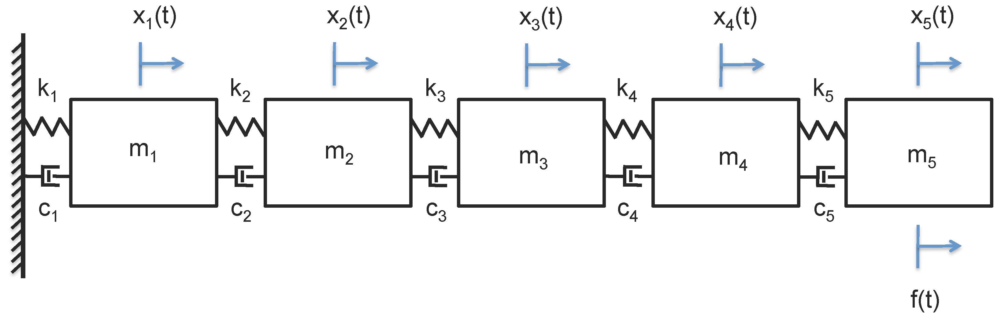
As an example, consider a five-DOF system governed by Equation (10), where:

$$\begin{array}{cc}\hfill \mathbf{M}& =\left[\begin{array}{ccccc}{m}_1& 0& 0& 0& 0\\ 0& m_2& 0& 0& 0\\ 0& 0& m_3& 0& 0\\ 0& 0& 0& m_4& 0\\ 0& 0& 0& 0& m_5\end{array}\right]\hfill \end{array}$$

$$\begin{array}{cc}\hfill \mathbf{C}& =\left[\begin{array}{ccccc}{c}_1+c_2& -c_2& 0& 0& 0\\ -c_2& c_2+c_3& -c_3& 0& 0\\ 0& -c_3& c_3+c_4& -c_4& 0\\ 0& 0& -c_4& c_4+c_5& -c_5\\ 0& 0& 0& -c_5& c_5\end{array}\right]\hfill \end{array}$$

$$\begin{array}{cc}\hfill \mathbf{K}& =\left[\begin{array}{ccccc}{k}_1+k_2& -k_2& 0& 0& 0\\ -k_2& k_2+k_3& -k_3& 0& 0\\ 0& -k_3& k_3+k_4& -k_4& 0\\ 0& 0& -k_4& k_4+k_5& -k_5\\ 0& 0& 0& -k_5& k_5\end{array}\right]\hfill \end{array}$$

(31)

are constant coefficient matrices commonly used to describe structural systems. In this case, these particular matrices describe the motion of a cantilevered structure where we assume a joint normally distributed random process applied at the end mass, i.e. $\mathbf{f}\left(t\right)=(0,0,0,0,\mathcal{N}(0,1\left)\right)$. In this first example we examine the TDTE between response data collected from two different points on the structure. We fix $m_i=0.01kg$, $c_i=0.1N·s/m$, and $k_i=10N/m$ for each of the $i=1\cdots 5$ degrees of freedom (thus we are using $\alpha =0.01$ in the modal damping model $\mathbf{C}=\alpha \mathbf{K}$). The system response data $x_i\left(n{\Delta }_t\right),n=1\cdots 2^{15}$ to the stochastic forcing is then generated via numerical integration. 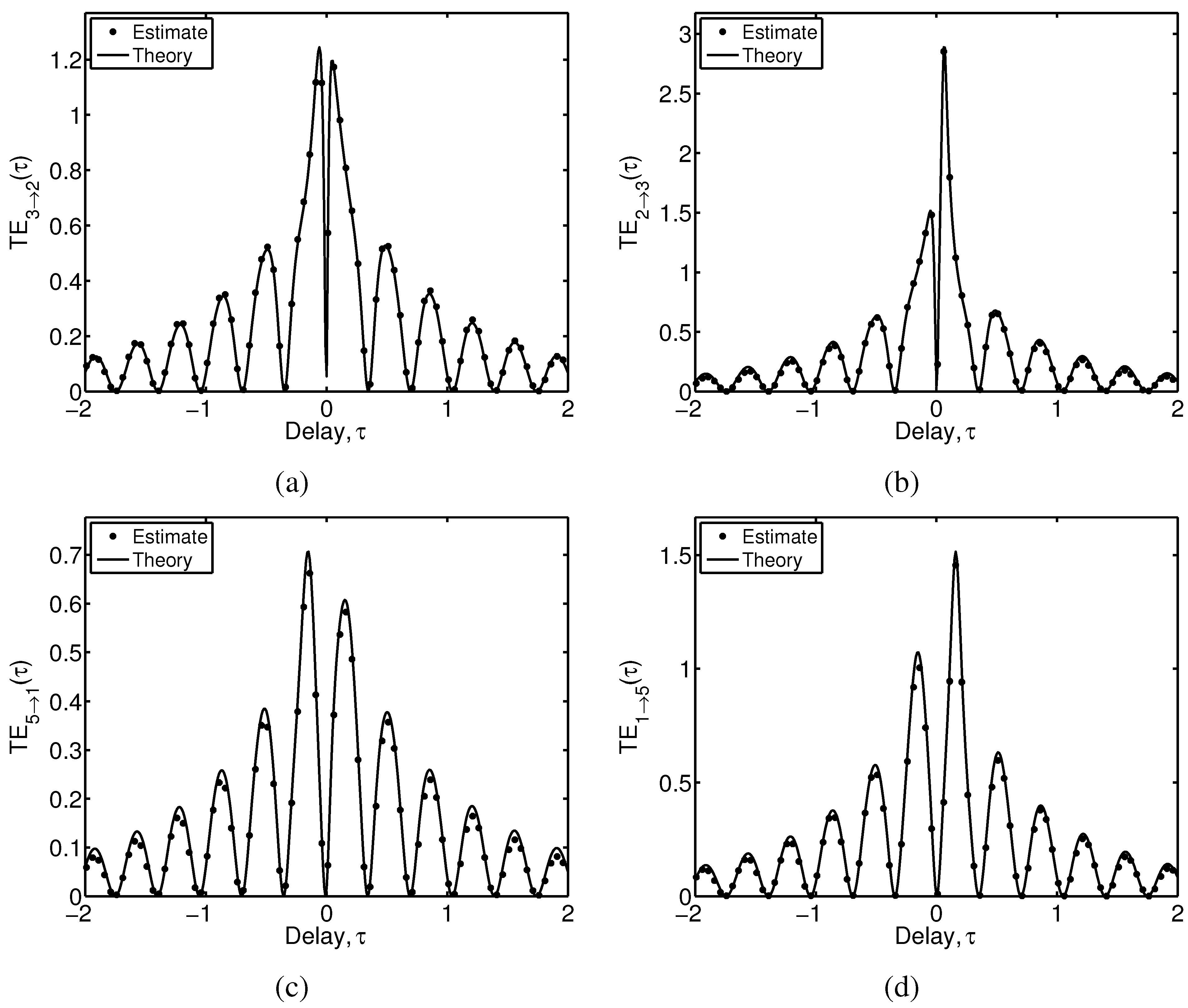For simulation purposes we used a time-step of ${\Delta }_t=0.01s$ which is sufficient to capture all five of the system natural frequencies (the lowest of which is ${\omega }_1=9.00$ rad/s). Based on these parameters, we generated the analytical expressions $T{E}_{3\to 2}\left(\tau \right)$ and $T{E}_{2\to 3}\left(\tau \right)$ and also $T{E}_{5\to 1}\left(\tau \right)$ and $T{E}_{1\to 5}\left(\tau \right)$ for illustrative purposes. These are shown in Figure 2 along with the estimates formed using the Fourier transform-based procedure. In forming the estimates we used $L=0$, $S=2^3$, $N_s=2^{12}$, resulting in low bias and variance, and providing curves that are in very close agreement with theory.

With Figure 2 in mind, first consider negative delays only where $\tau <0$. Clearly, the further the random variable $X_j(t_n+\tau )$ is from $X_i\left(t_n\right)$, the less information it carries about the probability of $X_i$ transitioning to a new state ${\Delta }_t$ seconds into the future. This is to be expected from a stochastically driven system and accounts for the decay of the transfer entropy to zero for large $\left|\tau \right|$. However, we also see periodic returns to the point $T{E}_{j\to i}\left(\tau \right)=0$ for even small temporal separation. Clearly this is a reflection of the periodicity observed in second order linear systems. In fact, for this system the dominant period of oscillation is $2\pi /{\omega }_1=0.698$ seconds. It can be seen that the argument of the logarithm in Equation (8) periodically reaches a minimum value of unity at precisely half this period, thus we observe zeros of the TDTE at times $(i-1)\times \pi /{\omega }_1,i=1\cdots$. In this case the TDTE is going to zero not because the random variables $X_j(t_n+\tau ),X_i\left(t_n\right)$ are unrelated, but because knowledge of one allows us to exactly predict the position of the other (no additional information is present). We believe this is likely to be a feature of most systems possessing an underlying periodicity and is one reason why using the TE as a measure of coupling must be done with care.

Figure 2. Time delay transfer entropy between masses two and three (top row) and one and five (bottom row) of a 5 DOF system driven at mass, $P=5$.

Figure 2. Time delay transfer entropy between masses two and three (top row) and one and five (bottom row) of a 5 DOF system driven at mass, $P=5$.

One possible way to eliminate this feature is to condition the measure on more of the signal’s past history. In fact, several papers (see e.g., [9,13]) mention the importance of conditioning on the full state vector $X_j(t_n-{\tau }_1),X_j(t_n-{\tau }_2),\cdots ,X_j(t_n-{\tau }_d)$ where d is the dimensionality (in a loose sense, the number of dynamical degrees of freedom) of the random process $X_j$. Building in more past history would almost certainly remove the oscillations as some of the past observations would always be providing additional predictive power. However, building in more history significantly complicates the ability to derive closed-form expressions. Moreover, for this simple linear system the basic envelope of the TDTE curves would not likely be effected by altering the model in this way.

We also point out that values of the TDTE are non-zero for positive delays as well. Again, so long as we interpret the TE as a measure of predictive power this makes sense. That is to say, future values $X_j$ can aid in predicting the current dynamics of $X_i$. Interestingly, the asymmetry in the TE peaks near $\tau =0$ may provide the largest clue as to the location of the forcing signal. Consistently we have found that the TE is larger for negative delays when mass closest the driven end plays the role of $X_j$; conversely it is larger for positive delays when the mass furthest from the driven end plays this role. So long as the coupling is bi-directional, results such as those shown in Figure 2 can be expected in general.

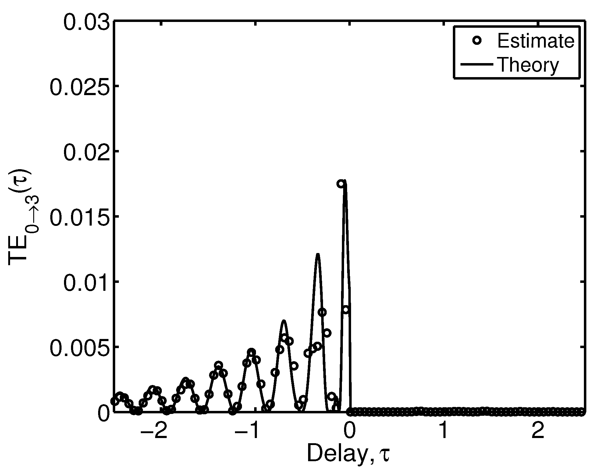
However, the situation is quite different if we consider the case of uni-directional coupling. For example, we may consider $T{E}_{f\to i}\left(\tau \right)$, i.e. the TDTE between the forcing signal and response variable i. This is a particularly interesting case as, unlike in previous examples, there is no feedback from DOF i to the driving signal. Figure 3 shows the TDTE between drive and response and clearly highlights the directional nature of the coupling. Past values of the forcing function clearly help in predicting the dynamics of the response. Conversely, future values of the forcing say nothing about transition probabilities for the mass response simply because the mass has not “seen” that information yet. Thus, for uni-directional coupling, the TDTE can easily diagnose whether $X_j$ is driving $X_i$ or vice-versa. It can also be noticed from these plots that the drive signal is not that much help in predicting the response as the TDTE is much smaller in magnitude that when computed between masses. We interpret this to mean that the response data are dominated by the physics of the structure (e.g., the structural modes), which is information not carried in the drive signal. Hence, the drive signal offers little in the way of additional predictive power. While the drive signal puts energy into the system, it is not very good at predicting the response. It should also be pointed out that the kernel density estimation techniques are not able to capture these small values of the TDTE. The error in such estimates is larger than these subtle fluctuations. Only the “linearized” estimator is able to capture the fluctuations in the TDTE for small ($O\left({10}^{-2}\right)$) values.

Figure 3. Time delay transfer entropy between the forcing (denoted as DOF “0”) and mass three for the 5 DOF system driven at mass, $P=5$. The plot is consistent with the interpretation of information moving from the forcing to mass three.

Figure 3. Time delay transfer entropy between the forcing (denoted as DOF “0”) and mass three for the 5 DOF system driven at mass, $P=5$. The plot is consistent with the interpretation of information moving from the forcing to mass three.

It has been suggested that the main utility of the TE is to, given a sequence of observations, assess the direction of information flow in a coupled system. More specifically, one computes the difference $T{E}_{i\to j}-T{E}_{j\to i}$ with a positive difference suggesting information flow from i to j (negative differences indicating the opposite) [2,4]. In the system modeled by Equation (10) one would heuristically understand the information as flowing from the drive signal to the response. This is certainly reinforced by Figure 3. However, by extension it might seem probable that information would similarly flow from the mass closest the drive signal to the mass closest the boundary (e.g., DOF 5 to DOF 1).

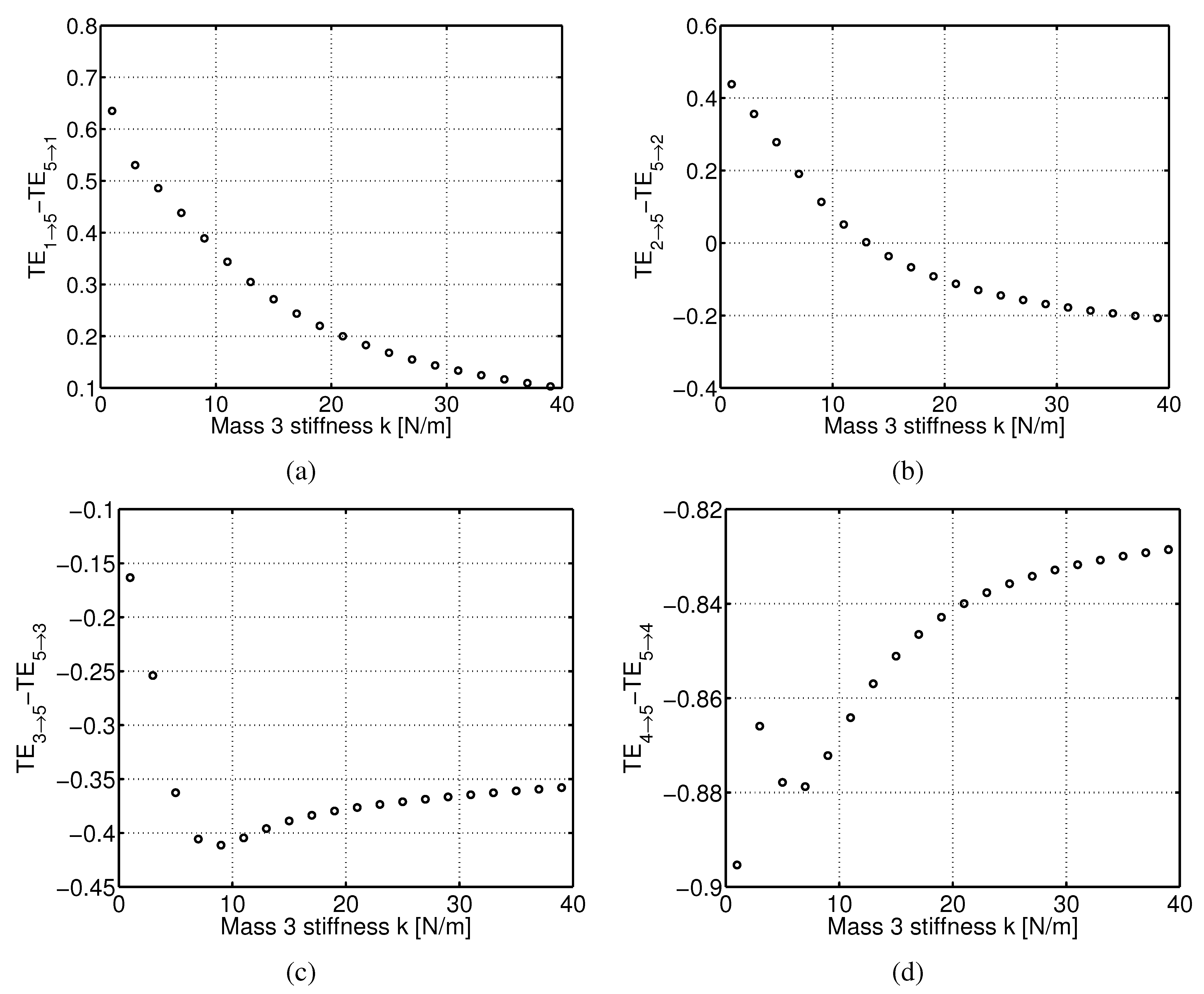
Figure 4. Difference in time delay transfer entropy between the driven mass five and each other DOF as a function of $k_3$. A positive difference indicates $T{E}_{i\to j}>T{E}_{j\to i}$ and is commonly used to indicate that information is moving from mass i to mass j. Based on this interpretation, negative values indicate information moving from the driven end to the base; positive values indicate the opposite. Even for this linear system, choosing different masses in the analysis can produce very different results. In fact, $T{E}_{2\to 5}-T{E}_{5\to 2}$ implies a different direction of information transfer, depending on the strength of the coupling, $k_3$

Figure 4. Difference in time delay transfer entropy between the driven mass five and each other DOF as a function of $k_3$. A positive difference indicates $T{E}_{i\to j}>T{E}_{j\to i}$ and is commonly used to indicate that information is moving from mass i to mass j. Based on this interpretation, negative values indicate information moving from the driven end to the base; positive values indicate the opposite. Even for this linear system, choosing different masses in the analysis can produce very different results. In fact, $T{E}_{2\to 5}-T{E}_{5\to 2}$ implies a different direction of information transfer, depending on the strength of the coupling, $k_3$

We test this hypothesis as a function of the coupling strength between masses. Fixing each stiffness and damping coefficient to the previously used values, we vary $k_3$ from $1N/m$ to $40N/m$ and examine the quantity $T{E}_{i\to j}-T{E}_{j\to i}$ evaluated at ${\tau }^{*}$, taken as the delay at which the TDTE reaches its maximum. Varying $k_3$ slightly alters the dominant period of the response. By accounting for this shift we eliminate the possibility of capturing the TE at one of its nulls (see Figure 2). For example, in Figure 2 we see that ${\tau }^{*}=-0.15$ in the plot of $T{E}_{3\to 2}\left(\tau \right)$. Figure 4 shows the difference in TDTE as a function of the coupling strength. The result is non-intuitive if one assumes information would move from driven end toward the non-driven end of the system. For certain DOFs this interpretation holds, for others, it does not. Herein lies the difficulty in interpreting the TE when bi-directional coupling exists. This was also pointed out by Schreiber [1] who noted “Reducing the analysis to the identification of a “drive" and a “response" may not be useful and could even be misleading”. The above results certainly reinforce this statement.

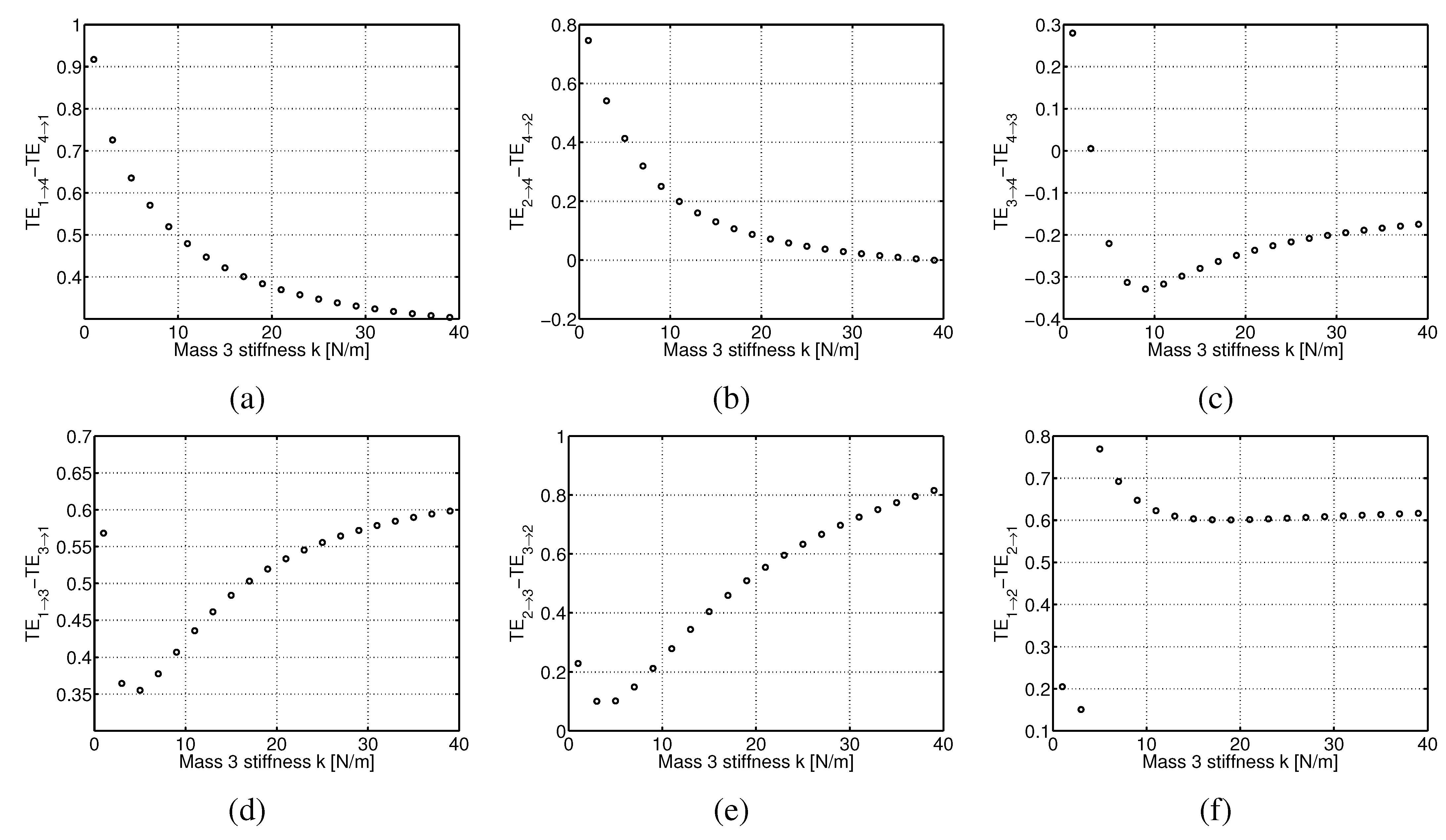
Figure 5. Difference in time-delayed transfer entropy (TDTE) among different combinations of masses. By the traditional interpretation of TE, negative values indicate information moving from the driven end to the base; positive values indicate the opposite.

Figure 5. Difference in time-delayed transfer entropy (TDTE) among different combinations of masses. By the traditional interpretation of TE, negative values indicate information moving from the driven end to the base; positive values indicate the opposite.

Rather than being viewed as a measure of information flow, we find it more useful to interpret the difference measure as simply one of predictive power. That is to say, does knowledge of system j help predict system i more so than i helps predict j. This is a slightly different question. Our analysis suggests that if $X_i$ and $X_j$ are both near the driven end but with DOF i the closer of the two , then knowledge of ${\mathbf{X}}_j$ is of more use in predicting ${\mathbf{X}}_i$ than vice-versa. This interpretation also happens to be consistent with the notion of information moving from the driven end toward the base. However as i and j become de-coupled (physically separated) it appears the reverse is true. The random process ${\mathbf{X}}_i$ is better at predicting ${\mathbf{X}}_j$ than ${\mathbf{X}}_j$ is in predicting ${\mathbf{X}}_i$. Thus, for certain pairs of masses information seems to be traveling from the base toward the drive. One possible explanation is that because the mass ${\mathbf{X}}_i$ is further removed from the drive signal it is strongly influenced by the vibration of each of the other masses. By contrast, a mass near the driven end is strongly influenced only by the drive signal. Because the dynamics ${\mathbf{X}}_i$ are influenced heavily by the structure (as opposed to the drive), ${\mathbf{X}}_i$ does a good job in helping to predict the dynamics everywhere. The main point of this analysis is that the difference in TE is not at all an unambiguous measure of the direction of information flow.

To further explore this question, we have repeated this numerical experiment for all possible combinations of masses. These results are displayed in Figure 5 where the same basic phenomenology is observed. If both masses being analyzed are near the driven end, the mass closest the drive is a better predictor of the one that is further away. However again, as i and j become decoupled the reverse is true. Our interpretation is that the further the process is removed from the drive signal, the more it is dominated by the other mass dynamics and the boundary conditions. Because such a process is strongly influenced by the other DOFs, it can successfully predict the motion for these other DOFs.

It is also interesting to note how the strength, and even directionality (sign) of the difference in TDTE changes with variations in a single stiffness element. Depending on the value of $k_3$ we see changes in which of the two masses is a better predictor. In some cases we even see zero TDTE difference, implying that the dynamics of the constituent signals are equally useful in predicting one another. Again, this does not support our intuitive notion of what it means for information to travel through a structural system. Only in the case of uni-directional coupling can we unambiguously use the TE to indicate directionality of information transport.

One of the strengths of our analysis is that these conclusions are not influenced by estimation error. In studying heart and breath rate interactions, for example, the ambiguity in information flow was assigned to difficulties in the estimation process [2]. We have shown here that even when estimation error is not a factor the ambiguity remains. We would imagine a similar result would hold for more complex systems, however such systems are beyond our ability to develop analytical expressions. The difference in TDTE is, however, a useful indicator of which system component carries the most predictive power about the rest of the system dynamics.

In short, the TDTE can be a very useful descriptor of system dynamics and coupling among system components. However any real understanding is only likely to be obtained in the context of a particular system model, or class of models (e.g., linear). Absent physical insight into the process that generates the observations, understanding results of a TDTE analysis can be challenging at best.

However, it is perhaps worth mentioning that the expressions derived here might permit inference about the general form of the underlying “linearized” system model. Different linear system models yield different expressions for ${\rho }_{ij}\left(\tau \right)$, hence different expressions for the TDTE. One could then conceivably use estimates of the TDTE as a means to select among this class of models given observed data. Whether or not the TDTE is of use in the context of model selection remains to be seen.

5. Conclusions

In this work we have derived an analytical expression for the time-delayed transfer entropy (TDTE) among components of a broad class of second order linear systems driven by a jointly Gaussian input. This solution has proven particularly useful in understanding the behavior of the TDTE as a measure of dynamical coupling. In particular, when the coupling is uni-directional, we have found the TDTE to be an unambiguous indicator of the direction of information flow in a system. However, for bi-directional coupling the situation is significantly more complicated, even for linear systems. We have found that a heuristic understanding of information flow is not always accurate. For example, one might expect information to travel from the driven end of a system toward the non-driven end. In fact, we have shown precisely the opposite to be true. Simply varying a linear stiffness element can cause the apparent direction of flow to change. It would seem a safer interpretation is that a positive difference in the transfer entropy between two system components tells the practitioner which component has the greater predictive power.

References

1. Schreiber, T. Measuring information transfer. Phys. Rev. Lett. 2000, 85, 461–464. [Google Scholar] [CrossRef] [PubMed]
2. Kaiser, A.; Schreiber, T. Information transfer in continuous processes. Phys. D: Nonlinear Phenom. 2002, 166, 43–62. [Google Scholar] [CrossRef]
3. Moniz, L.J.; Cooch, E.G.; Ellner, S.P.; Nichols, J.D.; Nichols, J.M. Application of information theory methods to food web reconstruction. Ecol. Model. 2007, 208, 145–158. [Google Scholar] [CrossRef]
4. Bauer, M.; Cox, J.W.; Caveness, M.H.; Downs, J.J.; Thornhill, N.F. Finding the direction of disturbance propagation in a chemical process using transfer entropy. IEEE Trans. Control Syst. Technol. 2007, 15, 12–21. [Google Scholar] [CrossRef]
5. Marschinski, R.; Kantz, H. Analysing the information flow between financial time series: An improved estimator for transfer entropy. Eur. Phys. J. B 2002, 30, 275–281. [Google Scholar] [CrossRef]
6. Nichols, J.M. Examining structural dynamics using information flow. Probab. Eng. Mech. 2006, 21, 420–433. [Google Scholar] [CrossRef]
7. Nichols, J.M.; Seaver, M.; Trickey, S.T.; Salvino, L.W.; Pecora, D.L. Detecting impact damage in experimental composite structures: An information-theoretic approach. Smart Mater. Struct. 2006, 15, 424–434. [Google Scholar] [CrossRef]
8. Moniz, L.J.; Nichols, J.D.; Nichols, J.M. Mapping the information landscape: Discerning peaks and valleys for ecological monitoring. J. Biol. Phys. 2007, 33, 171–181. [Google Scholar] [CrossRef] [PubMed]
9. Vicente, R.; Wibral, M.; Lindner, M.; Pipa, G. Transfer entropy-a model-free measure of effective connectivity for the neurosciences. J. Comput. Neurosci. 2001, 30, 45–67. [Google Scholar] [CrossRef] [PubMed]
10. Wibral, M.; Rahm, B.; Rieder, M.; Lindner, M.; Vicente, R.; Kaiser, J. Transfer entropy in magnetoencephalographic data: Quantifying information flow in cortical and cerebellar networks. Progr. Biophys. Mol. Biol. 2011, 105, 80–97. [Google Scholar] [CrossRef] [PubMed]
11. Vakorin, V.A.; Krakovska, O.A.; McIntosh, A.R. Confounding effects of indirect connections on causality estimation. J. Neurosci. Method. 2009, 184, 152–160. [Google Scholar] [CrossRef] [PubMed]
12. Barnett, L.; Barrett, A.B.; Seth, A.K. Granger causality and transfer entropy are equivalent for gaussian variables. Phys. Rev. Lett. 2009, 103, 238701. [Google Scholar] [CrossRef] [PubMed]
13. Palus, M.; Vejmelka, M. Directionality of coupling from bivariate time series: How to avoid false causalities and missed connections. Phys. Rev. E 2007, 75, 056211. [Google Scholar] [CrossRef] [PubMed]
14. Friston, K.J.; Harrison, L.; Penny, W. Dynamic causal modelling. NeuroImage 2003, 19, 1273–1302. [Google Scholar] [CrossRef]
15. Greenberg, M.D. Advanced Engineering Mathematics; Prentice-Hall, Inc.: Englewood Cliffs, NJ, USA, 1988. [Google Scholar]
16. Bendat, J.S.; Piersol, A.G. Random Data Analysis and Measurement Procedures, 3rd ed.; Wiley & Sons: New York, NY, USA, 2000. [Google Scholar]
17. Kay, S.M. Fundamentals of Statistical Signal Processing: Volume I, Estimation Theory; Prentice Hall: New Jersey, NJ, USA, 1993. [Google Scholar]
18. Meirovitch, L. Introduction to Dynamics and Control, 1st ed.; Wiley & Sons.: New York, NY, USA, 1985. [Google Scholar]
19. Crandall, S.H.; Mark, W.D. Random Vibration in Mechanical Systems; Academic Press: New York, NY, USA, 1963. [Google Scholar]
20. Benaroya, H. Mechanical Vibration: Analysis, Uncertainties, and Control; Prentice Hall: New Jersey, NJ, USA, 1998. [Google Scholar]
21. Nichols, J.M.; Olson, C.C.; Michalowicz, J.V.; Bucholtz, F. The bispectrum and bicoherence for quadratically nonlinear systems subject to non-gaussian inputs. IEEE Trans. Signal Process. 2009, 57, 3879–3890. [Google Scholar] [CrossRef]
22. Birkhoff, G.D. Proof of the ergodic theorem. Proc. Natl. Acad. Sci. USA 1931, 17, 656–660. [Google Scholar] [CrossRef] [PubMed]
23. Hahs, D.W.; Pethel, S.D. Distinguishing Anticipation from Causality: Anticipatory Bias in the Estimation of Information Flow. Phys. Rev. Lett. 2011, 107, 128701. [Google Scholar] [CrossRef] [PubMed]