Citizen Science and Topology of Mind: Complexity, Computation and Criticality in Data-Driven Exploration of Open Complex Systems

Abstract

Recently emerging data-driven citizen sciences need to harness an increasing amount of massive data with varying quality. This paper develops essential theoretical frameworks, example models, and a general definition of complexity measure, and examines its computational complexity for an interactive data-driven citizen science within the context of guided self-organization. We first define a conceptual model that incorporates the quality of observation in terms of accuracy and reproducibility, ranging between subjectivity, inter-subjectivity, and objectivity. Next, we examine the database’s algebraic and topological structure in relation to informational complexity measures, and evaluate its computational complexities with respect to an exhaustive optimization. Conjectures of criticality are obtained on the self-organizing processes of observation and dynamical model development. Example analysis is demonstrated with the use of biodiversity assessment database—the process that inevitably involves human subjectivity for management within open complex systems.

1. Introduction

Recent innovation of information and communication technologies (ICT) embedded in real environments is drastically changing the way society interacts with computation. This has been described as the fourth industrial revolution [1]. In particular, ubiquitous sensors and mobile communication tools have led to an increasing capacity of distributed and interactive environmental sensing. These technological supports bring in new effective methodologies to tackle complex self-organising behaviours in social–ecological systems that are difficult to understand with conventional modelling and simulation approaches (e.g., [2,3]). Massive amounts of sparse and heterogenous data that are based on the internal observation from within various collective phenomena call for an extended analytical framework, ranging from objective measurements (e.g., with sensors) to subjective data such as human evaluations and feedbacks.

Redefining a standard formalization of computation and its complexity that are associated with self-organised citizen science can raise multiple criteria for the evaluation of critical phenomena, spread over the dynamical process of observation, management, and knowledge formation in open complex systems [4,5]. Self-organised criticality appears in various natural and social phenomena, often with scale-free statistical properties [6,7]. They manifest in the power law, which can be reduced to a simple combination of inherent stochastic processes [8], and whose realizations provide proxies of emergent functionality (e.g., [9,10,11]). The large fluctuation of the power law distributes the statistical complexity in multiple scales that cannot be represented by a simple mean value for predictive purposes. The sampling time series from a power-law distribution encounters intermittent shifts of the sample average due to the infinite variance of distribution—even with the upper-bounded power law in the real world (e.g., in the magnitude distribution of earthquakes). This situation addresses a statistical limit of prediction solely by the modelling and simulation of the phenomena, but also presents a positive reason to engage human elements as a practical solution in actual management—especially those involving semantic and cognitive judgements [12,13]. On the technology side, machine learning models have long been attempting to optimize the prediction of unknown stochastic sources, implementing interactive estimation processes to exploit the hidden causal structure from temporal observation sequences (e.g., [14]). Modelling studies of guided self-organization have recently been explored with implementation in robotics, simulated neural networks, and networks of agents, etc. [15]. Although most of the achievement is discussed within the predictability of a confined experimental setting, a hybrid system with the synergy of human and computation elements always lies as a premise of real-world situation, which has been little exploited, except for some prototypical interfaces for the internet of things (e.g., [16]). For a cost-effective monitoring and control within restricted resources, guided criticality should be introduced to the user side of technology, in order to migrate and abstract decision making process from computation to human ability [3,4,17].

In particular, in solving global agendas such as sustainability goals, a comprehensive approach is required that should make use of the full potential of self-organisation in coupled social–ecological systems [5,18,19]. These efforts practically take on the engagement of citizens and multi-disciplinary stakeholders as important actors in the data acquisition and the implementation of an interactive management through guided self-organization, as a novel type of collective intelligence in the era of the fourth industrial revolution [3,20,21].

In facing the transition of data-driven citizen science towards the achievement of dynamical control in managing real-world open complex systems, this article raises fundamental theories and example models to support the discussion of complexity, computation, and criticality in its most possible general form. We formalize the basic objectives as follows, which are exploited in the subsequent sections with the corresponding numbers:

• Section 2: How can we formalize and treat the databases of varying quality from both machine and human observations, which range from subjective bias to objective fact? How can we set up scientific measures that should assure the compatibility with the principles of accuracy and reproducibility ?
• Section 3: How can we generalize the concept of complexity measures in application to the human–computer hybrid systems in citizen science?
• Section 4: What is the nature of computational complexities in actual data processing?
• Section 5: What is the general condition to yield guided self-organization for cost-effective citizen science?

Although these questions are universal in multiple industries, a common basis of understanding the problems and mutual development of ICT infrastructure are still isolated and developed independently in each sector. Throughout the exploration of these topics, this paper attempts to provide a common terminology and establish a theoretical basis for the realisation of a cost-effective citizen science in open complex systems situations. This is becoming increasingly important for solving transdisciplinary problems through the participation of multiple stakeholders in the real world [5].

2. Inter-Subjective Objectivity Model

We first consider the expression of the quality of data ranging between human subjectivity and machine objectivity in the general form of database $\mathbb{X}$. As a premise, any information that can be represented in digital computing is compatible with the natural number theory. At the infinite limit of computational memory, the representation of the database extends to general sets on a real data type with countably infinite precision, which accepts the definition of $\sigma$-finite measure in a measure-theoretical formulation. We define the general form of arbitrary database $\mathbb{X}$ as follows:

$$\begin{array}{c}\hfill \mathbb{X}={\mathbb{R}}^n\times {\mathbb{S}}^m(n,m\in \mathbb{N}).\end{array}$$

(1)

where $\mathbb{R}$ is a real data type, ${\mathbb{S}}^m$ is the m sets ${\{S_i\}}_{i=1,2,\cdots ,m}$ of arbitrary symbolic set $S_i=\{s_1,s_2,\cdots ,s_{l_i}\}$, with the dimensions n, m, and $l_i$ as natural numbers $\mathbb{N}$ including 0. Any variable in this article takes the assumption that it can be stored in $\mathbb{X}$. For mathematical simplicity, we hereafter consider the real data type $\mathbb{R}$ as a real number. In practice, ${\mathbb{R}}^n$ describes the values of n real variables (such as time, spatial coordinates, probabilities, etc.), and ${\mathbb{S}}^m$ represents m discrete sets of symbols (such as the name of variables, occurrence of discrete variables, text data, etc.). Obviously, ${\mathbb{S}}^m\subseteq {\mathbb{R}}^m$ holds in mathematical simplification, but we separate the notations to distinguish between the quantitative and qualitative variable types.

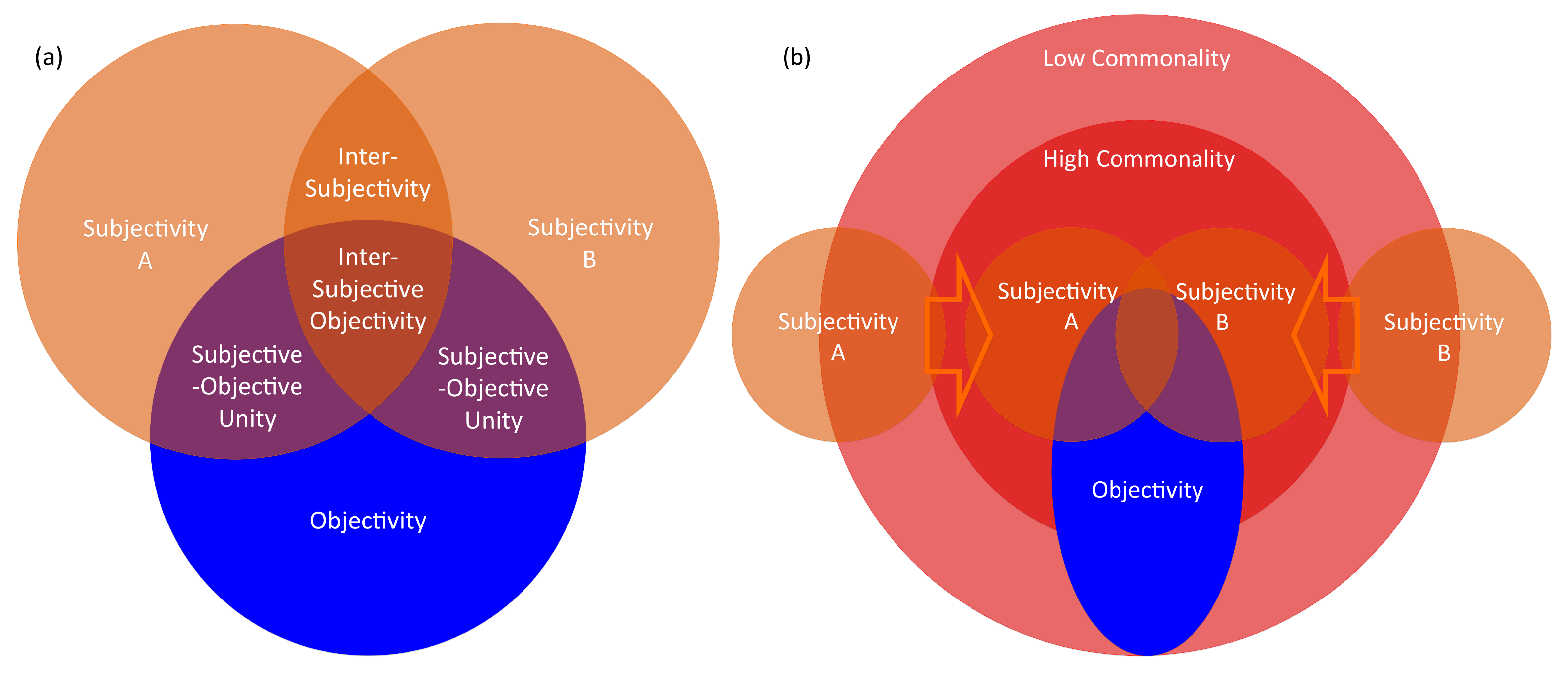
2.1. Formalization of Subjectivity, Inter-Subjectivity, Subjective–Objective Unity, and Objectivity

Digital data $\mathbb{X}$ from citizen science vary from subjective human perception to objective sensor measurement with a different degree of human-induced bias. Here, the subjectivity and objectivity matter because they influence the accuracy and reproducibility of data that is fundamental to establishing scientific analysis. We formalize the nature of observation variables between the subjectivity, objectivity, and these interactions as follows:

• Subjectivity is the quality of observation that is based on human perception without the substantial support of a machine.
• Inter-Subjectivity is the degree of commonality between the subjectivities of multiple subjects.
• Objectivity is the quality of observation that is based on a machine measurement whose consequence does not depend on the operator’s will.
• Subjective–Objective Unity is the degree of commonality between the subjectivity and objectivity.
• Inter-Subjective Objectivity is the quality of observation that satisfies the coincidence of both inter-subjectivity and subjective–objective unity.

These follow basic concepts in philosophy and social science and are adapted to the situation of data analysis. The concept of subjectivity is commonly used in philosophy as the collection of the perceptions, experiences, expectations, personal or cultural understanding, and beliefs specific to a person, which influences, informs, and is biased towards people’s judgments and evaluations. In contrast, objectivity refers to a view of truth or reality which is free from any individual’s influence [22]. The most simplistic form of inter-subjectivity in social science employs the term in the sense of having a shared definition of an object, or shared subjectivity [23].

The relations between these classifications are shown in Figure 1a. For example, text data written by humans are subjective data whether the fact described is based on an objective phenomenon or not. Sensor logs are objective data, even measured on a human body such as heart rate that could be influenced by subjective thought. When multiple subjects give the same subjective evaluation, such as rating of web contents, the commonality augments the degree of inter-subjectivity, which is often adapted to cloud-sourced data validation (e.g., [24,25]). When a subjective evaluation coincides with an objective measurement, the commonality represents the degree of subjective–objective unity. A highly reproducible subjective–objective unity can provide on-site practical measurement in field science, typical in biodiversity assessment and soil texture analysis (e.g., [25,26]). This is because these plausible subjective–objective unity measures also coincide with high inter-subjectivity after sufficient training, which guarantees the accuracy of on-site application without confirming the accordance with objective measurement each time. When the methodology is highly established with respect to the accuracy and reproducibility, it belongs to inter-subjective objectivity, where each subjective and objective measurement converges to the same result. The developmental process of reproducible subjective evaluations that converge with objective measurements is depicted in Figure 1b). By training the subjective–objective unity of each human observer, their inter-subjectivity increases, and the commonality of measurement augments to become a self-organizing loop between the subjective–objective unity and inter-subjectivity by a mutual feedback to attain a higher degree of inter-subjective objectivity.

Note that in a philosophical generalization (e.g., phenomenology), all data are the derivatives of subjectivity, because a machine observation is also constructed on human perception in the establishment of measurement principle, construction of sensing devices and data processing workflows, and final interpretation. To avoid trivial argument that does not affect the reproducibility of the results, we adopt the standpoint that separates the subjectivity and objectivity with the degree of intervention to observation outcome between human and machine. We call this conceptual model the inter-subjective objective model.

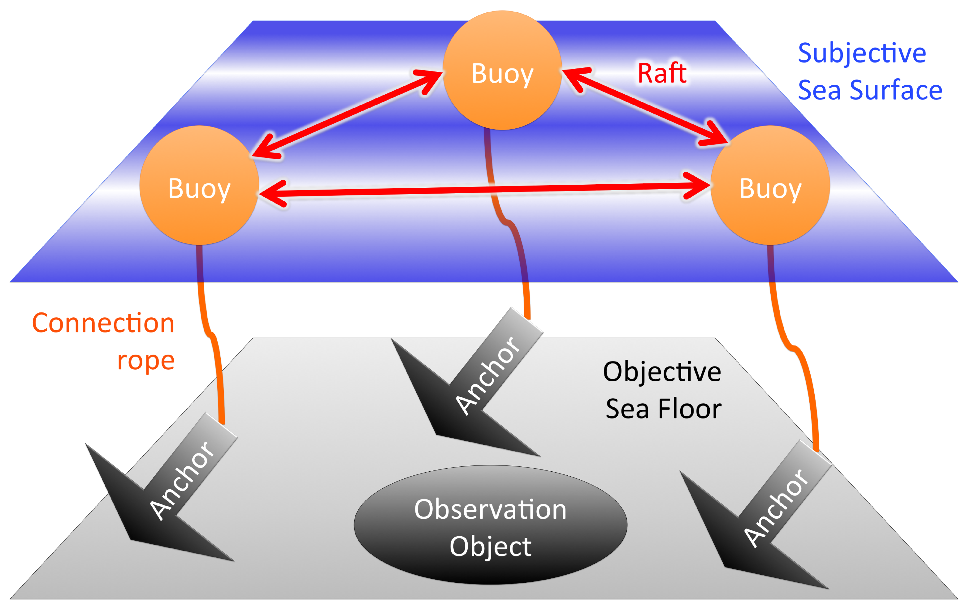
2.2. Representative Model: Buoy–Anchor–Raft Model

In order to apply the inter-subjective objective model into a quantitative framework of actual data processing, we develop a general example model with a more familiar and analogical terminology that are intuitively easier to understand: the buoy–anchor–raft model, as schematically expressed in Figure 2. The definition and correspondence to the inter-subjective objectivity model are given as follows:

• Buoy refers to subjective data that fluctuates on the sea surface, representing subjectivity. Buoy can provide subjective estimates of an observation object lying on the objective sea floor, but the observation is biased by subjective fluctuations.
• Anchor refers to objective data that is fixed on the sea floor representing objectivity, without the influence from the subjective sea surface. Anchors can be connected to buoys, which provide the evaluation of subjective fluctuation with respect to objective machine measurements.
• Raft represents the relationship between buoys, and refers to inter-subjectivity of data without reference to anchors. A buoy can evaluate another buoy using relative difference of fluctuation on a subjective sea surface, and the overall commonality between buoys is represented as the raft. Nevertheless, it is based on an internal observation between buoys without an objective system of units, and is therefore susceptible to a global drift of collective standard.
• Buoy–Anchor connection rope defines the degree of subjective–objective unity. As a buoy’s movement is more controlled by its anchor, higher subjective–objective unity is assured.
• Raft–Anchor connection ropes define the degree of inter-subjective objectivity. In addition to the commonality between buoys represented as a raft, the effects of the global drift from subjective sea surface could be controlled with anchors within a plausible range of error with respect to the objective sea floor.

Concrete examples of the buoy, anchor, raft in various social systems and scientific domains are given in

Table 1. Examples of buoy, raft, and anchor in various social systems and scientific domains. Examples are not comprehensive, but a partial list of typical data from the recently increasing public availability.

	Economy	Judiciary	Biodiversity Record	Medical Treatment
Buoy	Demand, satisfaction	Sense of justice, guilt	Visual identification of species	Pain, psychological state
Raft	Price, exchange rate	Law, court decision	Identification with voting	Diagnosis, prescription
Anchor	Goods abundance	Evidential matter	DNA sequences	Physiological markers

. While inter-subjective objectivity is a conceptual framework that classifies the quality of observation, the buoy, anchor, and raft refer to actual constructs of databases implemented with ICT. The terms arose from the developmental process of management systems in open systems science [5], sharing the perspective with the transversal question of the grand challenge of AI research regarding the effective extraction of scientific knowledge out of heterogenous data of varying quality [27]. Without properly positioning the subjective background of the study, it is often the case that established knowledge with large-scale experiments and statistical analyses is revealed to be false in high-throughput discovery-oriented research, resulting in a null-field with statistically prevailing bias [28]. As shown in Table 1, conceptual problematics for the implementation of ICT in various fields can be mutually characterized with the use of the buoy–anchor–raft model. This means the ICT infrastructure can be applied and shared in a synergistic way across domains, which is beneficial, especially for open-source development advocated in complex systems science [21]. Recent development in the application programming interface for big data integration has increased the support for this challenge, which calls for a general theoretical framework of information processing that the buoy–anchor–raft model can provide (e.g., [29]).

We then consider a mathematical expression of the buoy–anchor–raft model in view of providing a simplified idea of computation with respect to the evaluation of inter-subjective objectivity. Recently emerging contexts of citizen science make use of buoys as important information sources, in contrast to objective science such as traditional physics, which is usually self-contained with anchors. Buoys fluctuate with human subjectivity, which is scientifically called bias. Suppose we cannot directly measure observation objects as anchors. This constraint does not necessarily arise from the observation principle but rather from the resource limitation: For example, a field evaluation of biodiversity mostly depends on human observation because massive DNA barcoding is too costly or even ineffective. So, the accuracy of buoy data should be evaluated with other buoy–anchor connections compatible with observation objects. By defining a buoy data $\mathbf{B}\subset \mathbb{X}$ and corresponding measurable anchor data $\mathbf{A}\subset \mathbb{X}$, a buoy–anchor connection $\mathbf{C}$ can be defined as an error function $\mathrm{erf}(·)$ between $\mathbf{A}$ and $\mathbf{B}$:

$$\mathbf{C}:=\mathrm{erf}(\mathbf{B},\mathbf{A}).$$

(2)

In case of n observation objects $\mathbf{A}=(a_1,a_2,\cdots ,a_n)\in {\mathbb{R}}^n$ and $\mathbf{B}=(b_1,b_2,\cdots ,b_n)\in {\mathbb{R}}^n$ for one observer, a typical example of buoy–anchor connection $c\in \mathbb{R}$ is given with the regularized mean squared error:

$$c=\frac{1}{n}\sum _{i=1}^n{\left(\frac{a_i-b_i}{a_i}\right)}^2.$$

(3)

The regularization makes c accessible to the canonical evaluation of confidence interval, such as t-test. As a generalization to m observers, let us describe

$$\mathbf{C}=\left(\begin{array}{c}{c}_1\\ c_2\\ ⋮\\ c_m\end{array}\right),$$

(4)

where

$$c_j=\frac{1}{n}\sum _{i=1}^n{\left(\frac{a_{ij}-b_{ij}}{a_{ij}}\right)}^2,(j=1,2,\cdots ,m),$$

(5)

given that

$$\mathbf{A}=\left(\begin{array}{ccc}{a}_{11}& \cdots & a_{1m}\\ ⋮& \ddots & ⋮\\ a_{n1}& \cdots & a_{nm}\end{array}\right),\mathbf{B}=\left(\begin{array}{ccc}{b}_{11}& \cdots & b_{1m}\\ ⋮& \ddots & ⋮\\ b_{n1}& \cdots & b_{nm}\end{array}\right).$$

(6)

Next, we consider the raft model. In most social systems, the case-wise precise measurement of anchors is impossible, and we call for the raft of common sense and other social feedbacks as a premise of plausible judgement. Consider m observers with somehow quantifiable opinions (buoy) on n observation objects. We define the raft matrix $\mathbf{R}$ as follows, as a generalization of buoy data to m observers and n observation objects:

$$\mathbf{R}=\left(\begin{array}{ccc}{r}_{11}& \cdots & r_{1m}\\ ⋮& \ddots & ⋮\\ r_{n1}& \cdots & r_{nm}\end{array}\right),$$

(7)

where the raft by definition refers to the commonality contained between these buoys. In a completely equal society where every observer’s opinion is equally respected, we obtain the mean inter-subjective evaluation $\mathbf{E}=(e_1,\cdots ,e_n)$ on n objects as follows:

$$\mathbf{E}:=\left(\begin{array}{c}{e}_1\\ ⋮\\ e_n\end{array}\right)=\left(\begin{array}{ccc}{r}_{11}& \cdots & r_{1m}\\ ⋮& \ddots & ⋮\\ r_{n1}& \cdots & r_{nm}\end{array}\right)\left(\begin{array}{c}1/n\\ ⋮\\ 1/n\end{array}\right).$$

(8)

Decision-making based on the evaluation of raft can represent the community’s mean quantifiable opinions, although it is not free from collective bias. It remains only within the framework of inter-subjectivity. For a better evaluation in terms of inter-subjective objectivity, we need to introduce a connection with anchors. Let us introduce a buoy–anchor connection $\mathbf{C}$ from Equation (4), then an example of the inter-subjective objective evaluation ${\mathbf{E}}^{\prime }=(e_1^{\prime },\cdots ,e_n^{\prime })$ in the sense of raft–anchor connection can be given by:

$${\mathbf{E}}^{\prime }:=\left(\begin{array}{c}{e}_1^{\prime }\\ ⋮\\ e_n^{\prime }\end{array}\right)\propto \left(\begin{array}{ccc}{r}_{11}& \cdots & r_{1m}\\ ⋮& \ddots & ⋮\\ r_{n1}& \cdots & r_{nm}\end{array}\right)[-log(\mathbf{C})],$$

(9)

where

$$[-log(\mathbf{C})]=\left(\begin{array}{c}-log(c_1)\\ ⋮\\ -log(c_m)\end{array}\right).$$

(10)

This means that the error function of the buoy–anchor connection is reflected as an entropy that represents subjective–objective unity of each observer. The opinion of the observer with higher subjective–objective unity is weighted according to the informational scarcity of subjective errors. Such integrated evaluation incorporating the scoring system on observers’ quality are one of the general solutions in web-based citizen science (e.g., [25]).

Note that the n objects of observation can also coincide with m observers themselves. As $\mathbf{C}$ can be independently obtained from $\mathbf{R}$, it can also accept subjective objects of observation where direct anchors do not exist, such as psychological state or the quantification of qualia such as Quality Function Deployment (QFD) [30] and pain scale [31]. In such cases, traditional methods only employ simple raft evaluation $\mathbf{E}$ without anchors, as formalized in Equation (8). In contrast, with the buoy–anchor–raft model, it is possible to relate indirect anchors to other related objectively quantifiable variables, by expanding the database into a more comprehensive system. In either case, this model provides accessibility to the inter-subjective objective evaluation by properly defining the buoy, anchor, raft and its connections.

The correspondence between the buoy–anchor–raft model and computational variables developed in the following sections are listed in

Table 2. Correspondence between buoy–anchor–raft model and computational variables in this article.

Section Number	2.2	3.1	3.2	3.3	3.4	4	5
Buoy	$\mathbf{B}$	$\mu (·)$,$I(·)$	${\mu }_i(·)$,$q_i(·)$	Data contained in vertices V	Com. order I and $II$between N objects	Observations A, B, C, D, E	$P(·)$, $P_a(·)$, $P_s(·)$, $P_l(·)$, $P_o(·)$, $H^{\prime }$
Anchor	$\mathbf{A}$
Raft	$\mathbf{R}$, $\mathbf{E}$	${\mu }^{\prime }(·,·)$, $I_2(·,·)$	${\lambda }_N(·)$	Edge attribute of E	Com. order I and $II$ b/w N observers, TDC, I-I and I-N res. dim.	$O(·)$	$H_2^{\prime }$, $D^m(·:·)$, $D^e(·:·)$
Buoy–Anchor	$\mathbf{C}$
Raft–Anchor	${\mathbf{E}}^{\prime }$

.

3. Complexity Measures

We consider the generalization of complexity measures with respect to essential information processing in citizen science, based on the inter-subjective objectivity model with buoy–anchor–raft constructs. The concept and definition of complexity vary according to the fields, such as algorithmic complexity, statistical complexity, biological complexity, etc. In this paper, we take a generalized definition of complexity measure as the projection from a system’s variables to one-dimensional quantity, which is composed to express a distinctive characteristic of the system [32]. This includes classical indices mentioned with the context of complexity, as well as various forms of information expressed as numbers in ICT, such as feature dimensions of machine learning.

3.1. Complexity Measure and Search Function

We consider general forms of complexity defined on database $\mathbb{X}$ in relation to the search function. Complexity measures are widely studied in information theory, with the underlying principle to abstract a low-dimensional representative index of useful features for functional characterization of complex systems [32]. Usually, complexity measures defined on n real variables are the epimorphism to the one-dimensional real number line, ${\mathbb{R}}^n\mapsto \mathbb{R}$. The general complexity measure for citizen science is therefore the projection of the database to real value index, $\mathbb{X}\mapsto \mathbb{R}$, with the condition that this transformation will provide some utility for the management.

The importance of utility depends on the need for information retrieval in citizen science process, or the conditions that are practically used in a database search. Indeed, the search function is actually the retrieval of corresponding data set with respect to a given condition, such that

$$S_R[Q(x)]:=\{x\in \mathbb{X}|Q(x)\},$$

(11)

where $S_R$ stands for the search result on database $\mathbb{X}$ with search query $Q(·)$. For example, $Q(·)$ is an if–then construct that can specify the value range of real variables, or the matching with specific symbolic sequence, which returns the corresponding data sets into $S_R$.

In order to perform computation such as the calculation of the buoy–anchor–raft model evaluation, the integral I of $\sigma$-finite measure $\mu$ on $\mathbb{X}$ with respect to the condition $Q(·)$ can be defined as follows, with indicator function $\mathbf{1}(·|Q(·))$:

$$I(Q(x)):={\int }_{\mathbb{X}}\mathbf{1}(x|Q(x))\mu (dx),$$

(12)

where

$$\begin{array}{c}\hfill \mathbf{1}(x|Q(x)):=\left\{\begin{array}{ccc}1& if& x\in S_R[Q(x)],\\ 0& if& x\notin S_R[Q(x)].\end{array}\right.\end{array}$$

(13)

In one-dimensional case, $\mu$ can represent either of buoy or anchor. If we define $\mu :\mathbb{X}\mapsto \mathbb{R}$ as the function of occurrence probability $p(·)$ of $x\subset \mathbb{X}$, such as

$$\mu (x)=-p(x)log(p(x)),$$

(14)

then I coincides with entropy, one of the typical information theoretical complexity measures. $\mu$ can also include joint distribution, such that with ${\mu }^{\prime }$:

$$\begin{array}{c}\hfill \begin{array}{ccc}\hfill {\mu }^{\prime }(x,y)& =& {\displaystyle p(x,y)log\frac{p(x,y)}{p(x)p(y)},}\hfill \\ \hfill x& \ne & y,\hfill \\ \hfill x,y& \in & \mathbb{X},\hfill \end{array}\end{array}$$

(15)

in which case, the mutual information $I_2$,

$$\begin{array}{c}\hfill \begin{array}{ccc}\hfill I_2& :=& {\displaystyle {\int }_{\mathbb{X}}\mathbf{1}(x,y|Q(x),Q(y)){\mu }^{\prime }(dx,dy)}\hfill \end{array}\end{array}$$

(16)

can incorporate raft, buoy–anchor, and raft–anchor connections.

As a search query, $Q(x)$ provides a value of complexity measure I; we can also inversely use I to specify $S_R[Q(x)]$. We consider the invertible map $S_R^{-1}:\{x\in \mathbb{X}|I\}\to \{Q(x)\}$ that generates all possible queries $\{Q(x)\}$ which return the set of x associated with the given value of complexity measure I. For example, we can search the dataset with its entropy higher than a threshold $I_c$ by setting

$$\begin{array}{c}\hfill \{Q(x)\}:=S_R^{-1}\left[\left\{x\subset \mathbb{X}|{\int }_x\mu (dx)>I_c\right\}\right].\end{array}$$

(17)

Nevertheless, complexity measures that specifically define an arbitrary $Q(x)$ are generally not given explicitly. In practice, we usually compare the performance of known complexity measures with respect to the ability to characterize the features on which we focus our analysis. The general task is to invent a novel complexity measure that can exclusively separate patterns in $\mathbb{X}$, given implicitly as $Q(x)$. For that purpose, the following theorem holds:

Theorem 1.

For any search condition $Q(x)$, we can construct an exclusively selective complexity measure $I^{\prime }$ which can sort out effects from other variables, with the function $G(·):\mathbb{R}\mapsto \{Q(x)\}$, such that

$$\begin{array}{ccc}\hfill Q(x)& =& S_R^{-1}\left[\{x\in \mathbb{X}|I^{\prime }\}\right]=G(I^{\prime }),\hfill \end{array}$$

(18)

$$\begin{array}{ccc}\hfill I^{\prime }& =& G^{-1}(Q(x)).\hfill \end{array}$$

(19)

The definition of invertibility of G follows that of $S_R$.

Proofs of the theorems are given in Appendix A.

The intuitive geometric meaning of the inverse function relationship between complexity measures and search function is shown in Figure 3.

3.2. Observation Commonality as Complexity

Inter-subjective objectivity is based on the commonality among subjectivity, inter-subjectivity, and objectivity. Essential computation is therefore the search for commonality between different observation datasets, whether it be from humans or machines. We consider the observation commonality to be a complexity measure that conforms to inter-subjective objectivity, and analyze its general mathematical structure.

We consider $\sigma$-finite probabilistic measures ${\mu }_1$, ${\mu }_2$ on measurable database space $(\mathbb{X},\mathcal{B})$, where $\mathcal{B}$ stands for Borel $\sigma$-algebra of $\mathbb{X}$. Then, the convolution * of ${\mu }_1$ and ${\mu }_2$ is defined as follows:

$$\begin{array}{cc}\hfill {\mu }_1*{\mu }_2(s_i):=\sum _j{\mu }_2(s_j){\mu }_1(s_{i-j})& \mathrm{for}{s}_i\in \mathcal{B}(\mathbb{S}),\{s_i,s_j,s_{i-j}\}\in \mathbb{S},\end{array}$$

(20)

$$\begin{array}{cc}\hfill {\mu }_1*{\mu }_2(\mathbf{x}):={\int }_{\mathbb{R}}{\mu }_1(\mathbf{x}-y){\mu }_2(dy)& \mathrm{for}\mathbf{x}\in \mathcal{B}(\mathbb{R}),\mathbf{x}-y:=\{x-y|x\in \mathbf{x}\},\end{array}$$

(21)

where $\mathcal{B}(\mathbb{S})$ and $\mathcal{B}(\mathbb{R})$ represent $\sigma$-algebra of $\mathbb{S}\subset \mathbb{X}$ and $\mathbb{R}\subset \mathbb{X}$, respectively.

Through appropriate variable transformation, the convolution of probability measures with real type variables (21) can be expressed as follows, as the probability of the sum of the variables [33]:

$$\begin{array}{c}\hfill {\mu }_1*{\mu }_2(\mathbf{x})={\int }_{\mathbb{R}}{\int }_{\mathbb{R}}\mathbf{1}(x+y|x+y\in \mathbf{x}){\mu }_1(dx){\mu }_2(dy),\mathbf{x}\in \mathcal{B}(\mathbb{R}).\end{array}$$

(22)

By choosing finite sets of $\mathbf{x}$ such as time period, geographic range, and other real type variable range, as well as symbols for $\{s_i\}$ such as name of observation object, one can define the commonality of observations as a part of the convolution of the probabilities from different observers. The observation ${\mu }_1$ and ${\mu }_2$ can be of any nature between subjectivity, inter-subjectivity, and objectivity.

We now consider the condition of valid observation with respect to the regularization of probability measure as follows, for a general number of observers $i\in \{1,\cdots ,N\}$:

$$\begin{array}{c}\hfill {\int }_{\mathbb{R}}{\mu }_i(dx)=1.\end{array}$$

(23)

This means that by expanding the scale of the real type variable to infinity, one can observe its occurrence with probability 1. The same formalization also applies to $\sigma$-finite measure on $(\mathbb{S},\mathcal{B}(\mathbb{S}))$, which is integrated in the formalization with $(\mathbb{R},\mathcal{B}(\mathbb{R}))$.

Next, consider a confined variable range $r\subset \mathbb{R}$ with positive probability measure ${\mu }_i(r)>0$. This range can be of any complex form as long as it supports positive measure. In a real situation, this can correspond to intermittent observation time interval, scattered geographical range, and other discrete range of the real type variable. We define the rate of observation $q_i$ by observer i within variable range r as

$$\begin{array}{c}\hfill q_i(r):={\int }_{\mathbb{R}}\mathbf{1}(x|x\in r){\mu }_i(dx)\le 1,\end{array}$$

(24)

which converges to (23) with $r\to \mathbb{R}$.

The commonality of observation between two observers i, j based on r is expressed as the following convolution confined to r:

$$\begin{array}{c}\hfill \begin{array}{ccc}\hfill {\mu }_i*{\mu }_j(r_2)& :=& {\displaystyle {\int }_{\mathbb{R}}{\int }_{\mathbb{R}}\mathbf{1}(x+y|x+y\in r_2;x,y\in r){\mu }_i(dx){\mu }_j(dy)}\hfill \\ & =& {\displaystyle {\int }_{\mathbb{R}}{\int }_{\mathbb{R}}\mathbf{1}(x+y|x,y\in r){\mu }_i(dx){\mu }_j(dy)}\hfill \\ & =& {\displaystyle {\int }_r{\int }_r{\mu }_i(dx){\mu }_j(dy),}\hfill \\ \hfill r_2& :=& \{x_1+x_2|x_1,x_2\in r\},\hfill \end{array}\end{array}$$

(25)

which also means taking the sum of joint distributions ${\mu }_i·{\mu }_j$ between all smallest measurable events in r. The additional condition $x,y\in r$ in $\mathbf{1}(·)$ limits the integral of each variable within r, which includes formal condition $x+y\in r_2$. The following generalization holds:

Theorem 2.

For N independent and valid observation ${\mu }_i(r)>0$ $(i=1,\cdots ,N)$ on variable range $r\subset \mathbb{R}$, let

$$\begin{array}{c}\hfill \begin{array}{ccc}\hfill {\lambda }_N(r_N)& :=& {\mu }_1*{\mu }_2*\cdots *{\mu }_i*\cdots *{\mu }_N(r_N)\hfill \\ & :=& {\displaystyle {\int }_{{\mathbb{R}}^N}\mathbf{1}\left({\displaystyle \Lambda \sum _{i=1}^N{x}_i|\Lambda \sum _{i=1}^N{x}_i\in r_N;x_i\in r}\right)\prod _i^{\{1,\cdots ,N\}}{\mu }_i(d{x}_i)}\hfill \\ & =& {\displaystyle {\int }_{{\mathbb{R}}^N}\mathbf{1}\left({\displaystyle \Lambda \sum _{i=1}^N{x}_i|x_i\in r}\right)\prod _i^{\{1,\cdots ,N\}}{\mu }_i(d{x}_i),}\hfill \\ \hfill r_N& :=& \left\{{\displaystyle \Lambda \sum _{k=1}^N{x}_k|x_k\in r}\right\},\hfill \\ \hfill \Lambda & :=& \mathbb{R}\setminus \{0,\pm \infty \},\hfill \end{array}\end{array}$$

(26)

where the coefficient Λ is a free parameter that remains invariant under the convolution. Then

$$\begin{array}{c}\hfill {\lambda }_N(r_N)=\prod _i^N{q}_i(r).\end{array}$$

(27)

This means that the $N^{-1}$-th power of multiple convolution ${\lambda }_N(r_N)$ represents the geometric mean of N independent valid observation rates. By choosing regularization factor $\Lambda$, $r_N$ corresponds to the ensemble of possible mean values $\left({\displaystyle \Lambda =\frac{1}{N}}\right)$, integrated values $\left(\Lambda =1\right)$, and other weighted sum of N random samplings from r. The regularization parameter $\Lambda$ can further be generalized to an arbitrary measurable function $\Lambda (·)$ representing commonality characteristics, taking ${\displaystyle \sum _{i=1}^N{x}_i}$ as a variable.

With the use of the logarithmic scale, the information of ${\lambda }_N(r_N)$ is the sum of those with individual observation:

$$\begin{array}{c}\hfill -log({\mu }_1*{\mu }_2*\cdots *{\mu }_i*\cdots *{\mu }_N(r_N))=\sum _i^N(-log{\mu }_i(r)).\end{array}$$

(28)

As a similar property related to geometric mean, note that the following Young’s inequality also holds:

$$\begin{array}{c}\hfill |\Lambda |·||{\mu }_1*{\mu }_2*\cdots *{\mu }_i*\cdots {\mu }_N||\le \prod _i^N||{\mu }_i||,\end{array}$$

(29)

where $||·||$ denotes total variation. This assures us that the variation of the commonality remains within the order of the product of each observation’s variation.

However, it is important to note that as a general property of convolution,

$$\begin{array}{c}\hfill {\displaystyle {\lambda }_N(r)\ne \prod _i^N{q}_i(r).}\end{array}$$

(30)

The equality only holds in case $r\to \mathbb{R}$ or ${\mu }_i(r_N)={\mu }_i(r)$ for $i=1,\cdots ,N$, without implication for the independence of observations. For the convolution on general subset $r_s\subseteq r_N$, the exact definition is given by

$$\begin{array}{c}\hfill \begin{array}{ccc}{\lambda }_N(r_s)& :=& {\displaystyle {\int }_{{\mathbb{R}}^N}\mathbf{1}\left({\displaystyle \Lambda \sum _{i=1}^N{x}_i|\Lambda \sum _{i=1}^N{x}_i\in r_s;x_i\in r}\right){\mu }_1(d{x}_1)\cdots {\mu }_N(d{x}_N),}\hfill \end{array}\end{array}$$

(31)

though it requires direct calculation without relevance to $q_i(r)$. In order to obtain fast computable form, the following asymptotical generalization holds:

Theorem 3.

As $N\to \infty$, for $r\subset \mathbb{R}$, ${\mu }_i(r)>0$, $i=1,\cdots ,N$ and $r_s\subseteq r_N$, ${\lambda }_N(r_s)$ converges almost everywhere to the following:

$$\begin{array}{c}\hfill \begin{array}{ccc}{\lambda }_N(r_s)& \to & {\displaystyle {\int }_{r_s}\mathcal{N}(\Lambda {\nu }_N,{\Lambda }^2{\sigma }_N^2)m(dx)\times \prod _i^N{q}_i(r),}\hfill \end{array}\end{array}$$

(32)

where $m(·)$ is the Lebesgue measure on $\mathbb{R}$, and $\mathcal{N}({\nu }_N,{\sigma }_N^2)$ represents the normal probability density distribution with mean value ${\nu }_N$ and variance ${\sigma }_N^2$ as follows:

$$\begin{array}{c}\hfill \begin{array}{ccc}{\nu }_N& :=& {\displaystyle \sum _{i=1}^N{\int }_{\mathbb{R}}\mathbf{1}\left(x|x\in r\right)x{\mu }_i(dx),}\hfill \\ {\sigma }_N^2& :=& {\displaystyle \sum _{i=1}^N\left({\int }_{\mathbb{R}}\mathbf{1}\left(x|x\in r\right)x^2{\mu }_i(dx)-({\nu }_N^2-2{\nu }_N)\right)}\hfill \\ & \to & {\displaystyle \sum _{i=1}^N\left({\int }_{\mathbb{R}}\mathbf{1}\left(x|x\in r\right)x^2{\mu }_i(dx)-{\nu }_N^2\right).}\hfill \end{array}\end{array}$$

(33)

A numerical example of the convolution ${\lambda }_N(r_N)$ is presented in Figure 4. Theorems 2 and 3 can be directly generalized to ${\mathbb{R}}^n(n\in \mathbb{N})$, with $r\subset {\mathbb{R}}^d$.

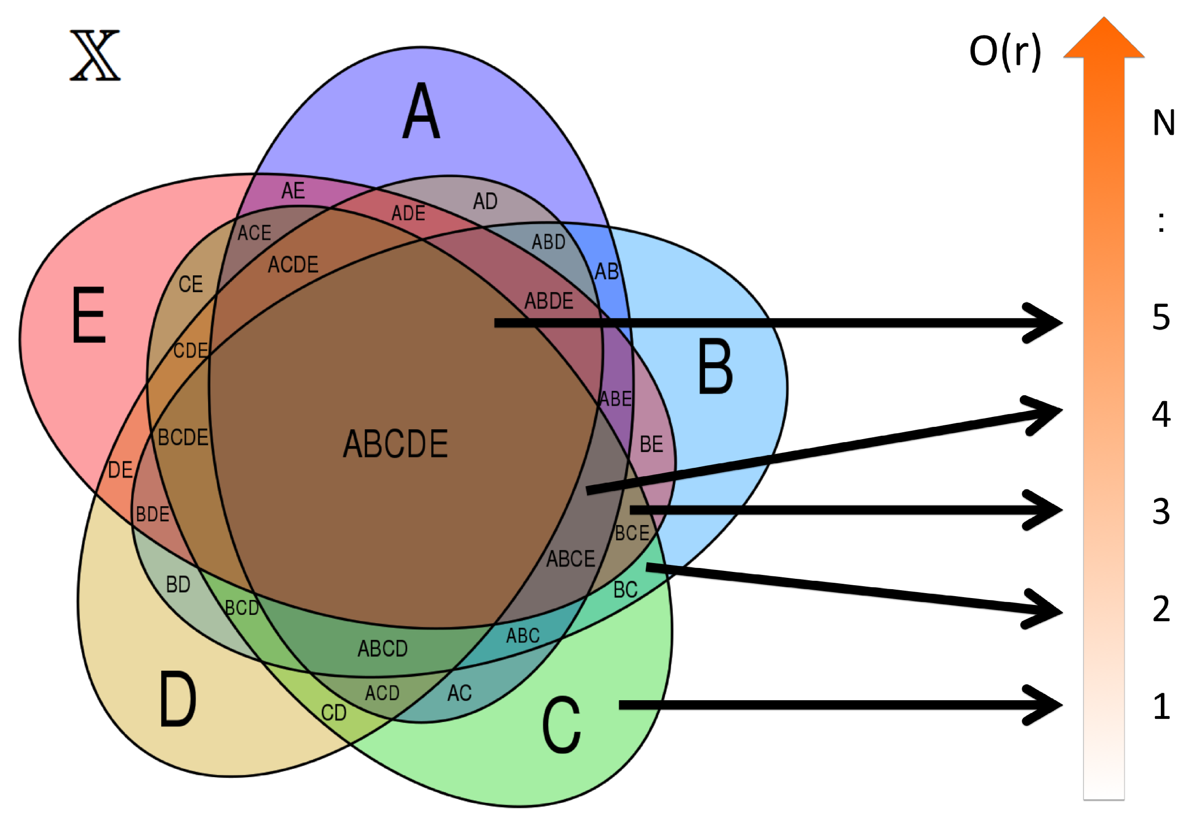
3.3. Topological Structure of Complexity 1: Total Order of Observations

We consider the topological structure of inter-subjective objectivity based on the complexity, defined as the convolution between different observations. As the commonality within inter-subjective objectivity is defined with multiple different observations, the topological ordering based on these complexity measures is possible with $N>2$ observations of any nature.

We consider the commonality space with respect to each observation dataset as a point, and commonality between them as the distance between each pair of points. This can be considered as the undirected complete graph with N vertices, and its pair-wise complexity measure as ${}_N{C}_2$ edges length. The general property of Euclidean space allows a complete graph of size N to be embedded in $N-1$ dimensions (e.g., any line between two points is one-dimensional space, and any triangle with three points is two-dimensional surface, etc.), although an additional quantitative restriction such as triangle inequality on each triplet of edges is required. In order to treat an arbitrary set of the complexity measures and yield general characteristics of commonality space, we need to focus not on the actual values of complexity, but on the topological order between them.

Let us first consider the total order between complexity values with $N>2$ observation data contained in N vertices $V:={\{v_i\}}_{i=1,\cdots ,N}$. One can determine the total order between ${}_N{C}_2$ edges $E:={\{e_k\}}_{k=1,\cdots ,{}_N{C}_2}:=\{v_i,v_{j\ne i}\in V\}$ by taking a mean order relationship between each pair of edges by the following algorithm (namely the pair-wise order algorithm):

• For each pair of edges $\{e_i,e_{j\ne i}\in E\}$, calculate the order relation $e_i\le e_j$ or $e_i\ge e_j$ with respect to the given complexity measure as an edge attribute such as length.
• Score each edge $e_i$ by mapping to integer $z:e_i\mapsto \mathbb{Z}$ by adding $+1$ if $e_i\ge e_{j\ne i}$ and by adding $-1$ if $e_i\le e_{j\ne i}$, with respect to all other edges $e_{j\ne i}$.
• The sorting with the score $\{z(e_i)\}$ provides the total order of E.

Note that the quantitative difference is completely lost in the case of antisymmetry, $(e_i=e_j)\equiv (e_i\le e_j)\wedge (e_i\ge e_j)$. We will consider the meaning of this information loss with respect to other compatible sets of observation in Section 3.4.

Next, we consider the topological order of complexity for $N>2$ observations according to the total order of these commonalities. We need here to translate the total order between edges E to that of observations V. This can be obtained by calculating the ${}_N{C}_3$ triplet of $N>2$ vertices and associated total order of edges with the following algorithm (namely, the triplet order algorithm schematically represented in Figure 5):

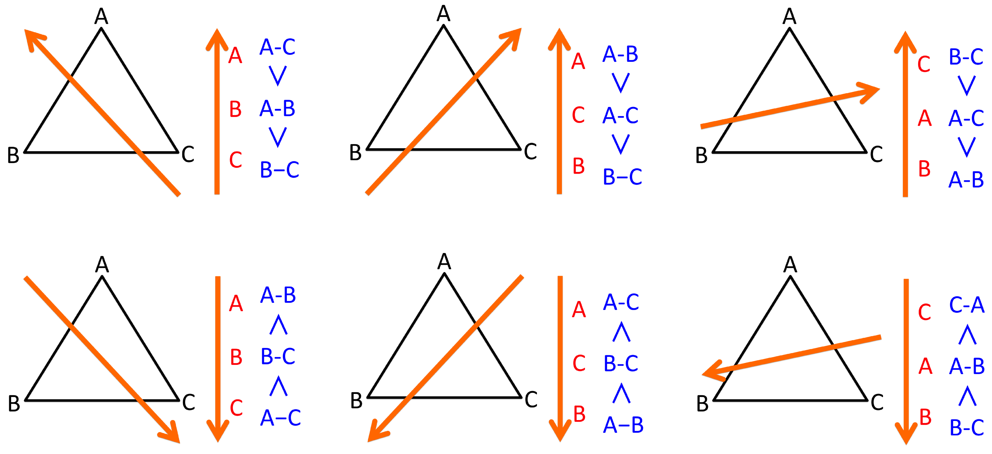
• For each triplet of observation $V_{i,j,k}:=\{v_i,v_{j\ne i},v_{k\ne i,j}\in V\}$ and associated edges $\{e_i:=\{v_i,v_j\},e_j:=\{v_j,v_k\},e_k:=\{v_k,v_i\}\}$, update score of each observation by mapping to integer $z^{\prime }:V_{i,j,k}\mapsto \mathbb{Z}$ with the following six rules:
• If $e_i\ge e_j\ge e_k$, then $z^{\prime }(v_i)=z^{\prime }(v_i)-1$, $z^{\prime }(v_j)=z^{\prime }(v_j)+1$, $z^{\prime }(v_k)=z^{\prime }(v_k)+0$.
• If $e_i\ge e_k\ge e_j$, then $z^{\prime }(v_i)=z^{\prime }(v_i)+1$, $z^{\prime }(v_j)=z^{\prime }(v_j)-1$, $z^{\prime }(v_k)=z^{\prime }(v_k)+0$.
• If $e_j\ge e_i\ge e_k$, then $z^{\prime }(v_i)=z^{\prime }(v_i)+0$, $z^{\prime }(v_j)=z^{\prime }(v_j)+1$, $z^{\prime }(v_k)=z^{\prime }(v_k)-1$.
• If $e_j\ge e_k\ge e_i$, then $z^{\prime }(v_i)=z^{\prime }(v_i)+0$, $z^{\prime }(v_j)=z^{\prime }(v_j)-1$, $z^{\prime }(v_k)=z^{\prime }(v_k)+1$.
• If $e_k\ge e_i\ge e_j$, then $z^{\prime }(v_i)=z^{\prime }(v_i)+1$, $z^{\prime }(v_j)=z^{\prime }(v_j)+0$, $z^{\prime }(v_k)=z^{\prime }(v_k)-1$.
• If $e_k\ge e_j\ge e_i$, then $z^{\prime }(v_i)=z^{\prime }(v_i)-1$, $z^{\prime }(v_j)=z^{\prime }(v_j)+0$, $z^{\prime }(v_k)=z^{\prime }(v_k)+1$.
• The sorting with the score $\{z^{\prime }(v_i)|i=1,\cdots ,N\}$ provides the total order of V.

The commonality order of V represents the topological structure of collective intelligence in citizen science with respect to inter-subjective objectivity, which corresponds to the topological inclusion relation of the Venn diagram in Figure 1.

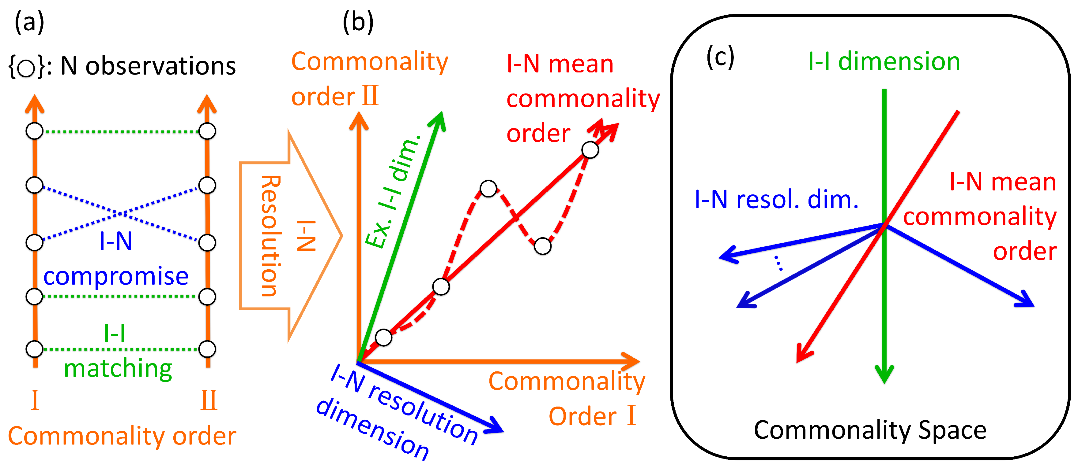
3.4. Topological Structure of Complexity 2: Permutation between Total Orders of Observations

We expand the situation to two sets of $N>2$ observations—namely, observation I and $II$. For example, observer I and $II$ observing N objects, or N observers observing 2 different objects I and $II$. It can also represent the application of two different complexity measures I and $II$ to N observations. For simplicity, we limit the formalization to two sets of $N>2$ observations, but generalization to a greater number of sets is possible.

In the general case, total orders I and $II$ do not necessarily coincide. The relationship between two total orders with N observations can be described with the permutation of N elements (Figure 6a). In order to analyze the permutation between total orders, let ${\mathcal{G}}_N$ be a symmetric group with degrees of N. For $g\in {\mathcal{G}}_N$, we define a linear transformation $L_g:{\mathbb{S}}^N\mapsto {\mathbb{S}}^N$ by

$$L_g:(v_1,\cdots ,v_N)\mapsto (v_{g(1)},\cdots ,v_{g(N)}),$$

(34)

which describes the permutation between commonality orders I and $II$.

We define a subspace ${\mathbb{S}}^{\prime }(g)$ of ${\mathbb{S}}^N$ by

$${\mathbb{S}}^{\prime }(g)=\{v_i\in \mathbb{S}|v_i\ne v_{g(i)}\},$$

(35)

which represents the subspace with compromise of total order. While by defining its complementary subspace

$${\mathbb{S}}^{\prime \prime }(g)=\{v_i\in \mathbb{S}|v_i=v_{g(i)}\},$$

(36)

we obtain the subspace in which there is no compromise, or the complete matching of two commonality orders. The whole commonality space can be divided into ${\mathbb{S}}^{\prime }(g)$ and ${\mathbb{S}}^{\prime \prime }(g)$:

$${\mathbb{S}}^N={\mathbb{S}}^{\prime }(g)\times {\mathbb{S}}^{\prime \prime }(g).$$

(37)

As depicted in Figure 6a,b, the compromise between two commonality orders is expressed as a non-linear folding relationship between them. Making the assumption that the complexity measure is a continuous function, the integrated complexity measure that supports both commonality orders can be expressed as a folded structure (topologically speaking), such as the shape of the letter “N” (also the capital letter of Non-identical), taking the commonality measure of I and $II$ as an affine coordinate: the example with a red dotted line in Figure 6b shows that we can compose an integrated commonality measure by bending the commonality measure $II$ in an “N” shape with respect to that of I kept straight (in “I” shape, for Identical), which resolves the compromise. The “N” shape transformation of commonality measure means to change the topology of commonality order with respect to a permutation $g\in {\mathcal{G}}_N$ $(g(i)>g(j),1\le i<j\le N)$, while that of “I” shape represents the identical order $(g(i)<g(j),1\le i<j\le N)$. The non-compromising part of the two commonality orders conserves its order to the projection onto any linear combination of the two commonality measures, which topologically do not require “N” shape folding, but maintain “I” shape matching.

For simplicity, We call the topological compromise between commonality orders the I–N compromise, and we call topologically identical matching I–I matching. Then, I–I matching subspace ${\mathbb{S}}^{\prime }(g)$ can be obtained as the linear combination of commonality measures I and $II$, and the subspace required for the resolution of I–N compromise corresponds to the complementary space ${\mathbb{S}}^{\prime \prime }(g)$ (Figure 6b,c).

We call ${\mathbb{S}}^{\prime }(g)$ an I–I space that consists of I–I dimensions, and ${\mathbb{S}}^{\prime \prime }(g)$ an I–N resolution space that consists of I–N resolution dimensions. The mean commonality order of two commonality orders projected onto I–I space (red solid arrows in Figure 6b,c) can be obtained with the use of the pair-wise order algorithm in Section 3.3, applied not to commonality itself, but to commonality orders. We call this the I–N mean commonality order, since it adopts the mean total order of commonality orders of I and $II$, resolving the I–N compromise. Note that the information lost by antisymmetry of the pair-wise order algorithm does not affect the division of I–I and I–N resolution subspaces. Geometrical representation of the I–N compromise, I–I matching, and these corresponding dimensions, spaces, and the I–N mean commonality order are given in Figure 6.

We finally consider a statistical test on the degree of coincidence (TDC) between 2 commonality orders.

Theorem 4.

Statistical test on the degree of coincidence (TDC) between two commonality orders:

Given that commonality orders I and $II$ with N observations follow a uniformly random permutation with ${\mathcal{G}}_N$ as null hypothesis, the degree of coincidence $d_c$ between the three commonality orders follows a binomial distribution:

$$\begin{array}{c}\hfill \begin{array}{ccc}{k}_{\mathrm{I}-\mathrm{I}}& :=& \#\{(i,j)|g(i)<g(j),1\le i<j\le N,g\in {\mathcal{G}}_N\},\hfill \\ P[d_c=k_{\mathrm{I}-\mathrm{I}}]& :=& {}_M{C}_{k_{\mathrm{I}-\mathrm{I}}}{p}^{k_{\mathrm{I}-\mathrm{I}}}{(1-p)}^{N-k_{\mathrm{I}-\mathrm{I}}}\hfill \\ & \sim & B(M,p),\hfill \end{array}\end{array}$$

(38)

where $B(M,p)$ signifies a binomial distribution of parameters $M={}_N{C}_2$ and $p=0.5$, $k_{\mathrm{I}-\mathrm{I}}$ represents the degree of coincidence as the number of I–I matching, $\#(·)$ returns the size of the set, and $P[·]$ the probability of the degree of coincidence $d_c$.

With respect to the buoy–anchor–raft model in Section 2.2, the following correspondence is possible:

• Two observers observing N objects: Commonality orders I and $II$ can correspond to either subjective (buoy) or objective (anchor) observation. The I–N resolution provides integrated commonality measure such as buoy–anchor connection and raft evaluation according to the nature of the observation. TDC provides connections between buoys and/or anchors.
• N observers observing two different objects: The commonality of N observers—whether it be subjective (buoy) or objective (anchor)—are ranked with respect to two different objects I and $II$. The I–N resolution provides a mean ranking of N observers’ commonality upon these observations. TDC provides the reproducibility of commonality among N observers.
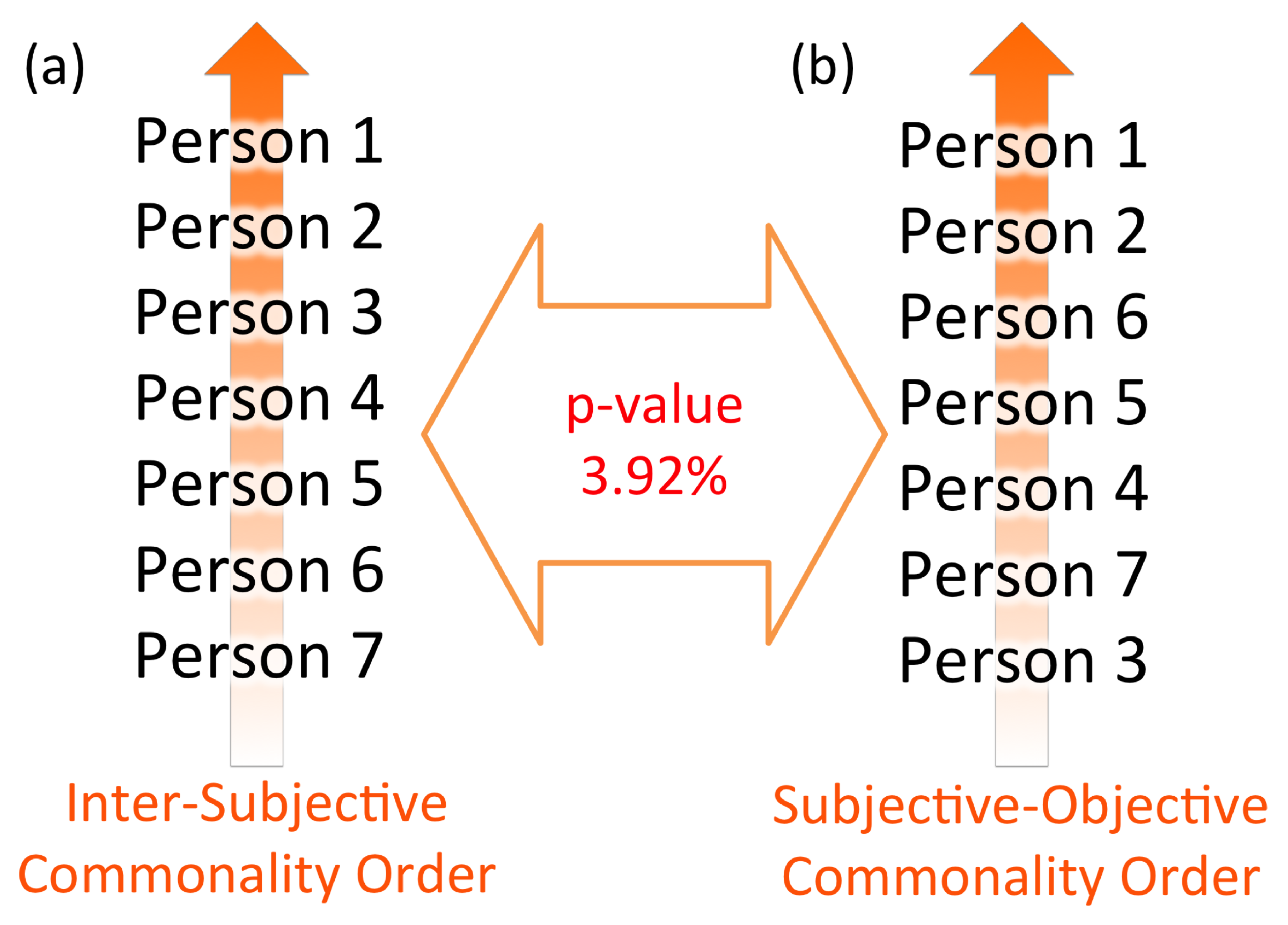
• Application of two different complexity measures to N observations: For example, the case of raft–anchor connection where N subjective observers (buoys) are ranked with inter-subjective commonality (raft evaluation) and weighted with two different anchors. The I–N resolution provides mean ranking of N observers’ inter-subjective objectivity, integrating multiple criteria of inter-subjective and objective evaluation. TDC represents statistical dependencies between two complexity measures in response to a given inter-subjective objective measurement. While significant matching between two commonality orders assures the reproducibility based on the coincidence of observation with these measures, non-significance can also be used to quantify complementarity of different evaluations [32].

4. Computational Complexity

The computation of complexity measures and commonality orders depends on the exhaustive calculation of combinatorics between observations. The computational complexity of such calculation should also be investigated in terms of topological complexity, in order to yield a general theoretical platform that does not depend on the particularity of the database.

4.1. Topological Complexity of Commonality

First, we investigate topological order of commonality among N observations. Using the convolution as commonality (27), we define the maximum commonality order $O:\mathbb{X}\mapsto \mathbb{N}$ as follows:

$$\begin{array}{c}\hfill O(r\subset \mathbb{X}):=max\{k\in 1,\cdots ,N|{\lambda }_k(r)>0\}.\end{array}$$

(39)

The general topological structure of $O(\mathbb{X})$ is depicted in Figure 7.

On the cardinality of $O(\mathbb{X})$, the following holds:

Theorem 5.

As $\#(\mathbb{X})\to {\aleph }_0$, ${}^{\exists }r\subset \mathbb{X}$ such that $\#(\{r|O(r)=\infty \})={\aleph }_0$, where ${\aleph }_0$ represents aleph-naught.

This means that for any elaborated inter-subjective objectivity, there is always the possibility to develop another different set of observations that attains higher inter-subjective objectivity by increasing the dataset. This structure assures the representation of a paradigm shift in science when sufficient contradicting evidence gained a majority compared to an old model. For example, minority reports in biology that may lead to novel discoveries in the future can be properly stored and distinguished from erroneous reports as more evidence accumulates [27].

4.2. Algorithmic Complexity

Secondly, we evaluate the computational complexity with respect to the computing time scale. Since data-driven citizen science requires real-time computation in a highly interactive manner with observation process, the algorithmic complexity of the calculation of complexity measures is an essential limiting factor of performance. As commonality is based on the intersection of multiple observations, its exhaustive computing confronts combinatorial explosion as datasets increase. Although computation of complexity itself, or resolution of search query as mathematical theorem is provable and an algorithmic solution can be found, the computation resource is another practical issue for real-world implementation—especially in distributed observation.

The computational time scale required for the sorting of a database according to a given utility such as commonality is listed in

Table 3. Algorithmic complexity for the calculation of commonality orders. With respect to the maximum commonality order in (39), an exhaustive number of combinations with the use of observation probability database ${\mathbb{X}}_N$ of size N and the time scale required for the sorting of the commonality measure is shown. Sorting time is based on the worst-case performance of canonical algorithms such as bubble sort and quick sort (polynomial degree $d=2$). $\mathcal{O}(·)$ denotes asymptotic notation of Landau. $O(\mathbb{X})=\lfloor \frac{N}{2}\rfloor$ and $\lceil \frac{N}{2}\rceil$ require the maximum calculation and sorting time. Note that the total computation time is upper-bounded by the sorting process ($d=2$) than the combinatorics of commonality ($d=1$), though calculation time of each commonality such as convolution should be further considered in actual implementation.

Maximum Commonality Order $\mathit{O}(\mathbb{X})$	Number of Combination	Sorting Time ($\mathit{d}=2$)
2	${}_N{C}_2$	$\mathcal{O}({({}_N{C}_2)}^2)=\mathcal{O}(N^4)$
3	${}_N{C}_3$	$\mathcal{O}({({}_N{C}_3)}^2)=\mathcal{O}(N^6)$
⋮	⋮	⋮
${\displaystyle \lfloor \frac{N}{2}\rfloor }$ or ${\displaystyle \lceil \frac{N}{2}\rceil }$	${}_N{C}_{\lfloor \frac{N}{2}\rfloor }$=${}_N{C}_{\lceil \frac{N}{2}\rceil }$	$\mathcal{O}\left({\left({}_N{C}_{\lfloor \frac{N}{2}\rfloor }\right)}^2\right)=\mathcal{O}\left({\left({}_N{C}_{\lceil \frac{N}{2}\rceil }\right)}^2\right)=\mathcal{O}\left(N^{2·\lfloor \frac{N}{2}\rfloor }\right)$
⋮	⋮	⋮
N	${}_N{C}_N=1$	$\mathcal{O}({({}_N{C}_N)}^2)=\mathcal{O}(1)$

. Under a general condition with the observation probability database ${\mathbb{X}}_N$ of size N, ${\mathbb{X}}_N:=\{{\mu }_i(x)|x\in \mathbb{X},i=1,\cdots ,N\}$, maximum complexity lies in the calculation of commonality order based on the intersection of ${\displaystyle \lfloor \frac{N}{2}\rfloor }$ or ${\displaystyle \lceil \frac{N}{2}\rceil }$ elements, whose sorting time belongs to factorial order of N . The case with $N=5$ is depicted in Figure 7. This means that an algorithmic burden exists towards the calculation of middle-scale commonality with respect to the data size. As an inter-subjective objectivity successfully increases in citizen science, this peaking of algorithmic complexity in intermediate scale may hinder the effective feedback necessary for guided self-organization.

However, in a practical situation, the actual computation time may remain in polynomial order if effective data size shrinks with respect to the increase of maximum commonality order:

Theorem 6.

By defining the diminution rate of data combination $\Delta :\mathbb{N}\mapsto \mathbb{R}$ with respect to maximum commonality order $1\le i\le N\in \mathbb{N}$ as

$$\begin{array}{c}\hfill \Delta (i):=\frac{{}_N{C}_{dim(\{{\mathbb{X}}_N|O(\mathbb{X})=i\})}}{{}_N{C}_{dim(\{{\mathbb{X}}_N|O({\mathbb{X}}_N)=i-1\})}}\end{array}$$

(40)

the order of its product is upper bounded by the d-th root of maximum computational complexity at ${\displaystyle N^{\prime }=\lfloor \frac{N}{2}\rfloor }$

$$\begin{array}{c}\hfill \prod _i^{N^{\prime }}\Delta (i)\le \sqrt[d]{\mathcal{O}(N^{d{N}^{\prime }})},\end{array}$$

(41)

where $dim(·)$ returns the size of the database, and $d>0$ represents the polynomial order of the algorithm $\mathcal{O}(N^d)$ with respect to the data size N.

From this result, we can conjecture that for $N^{\prime \prime }\le N^{\prime }$,

$$\begin{array}{c}\hfill \prod _i^{N^{\prime \prime }}\Delta (i)\le \mathcal{O}(N^{\frac{c}{d}})\end{array}$$

(42)

will assure exhaustive feedback with polynomial response time of degree c. Usually, the left side is based on the past calculation of lower maximum commonality order, we can annotate interactively whether interactive information processing can assure comprehensive feedback. This will add a criterion on the criticality of guided self-organization mediated by computation, which will be explored in Section 5.

Another methodology other than exhaustive computing is to implement a local gradient algorithm as a local interaction that leads to a global heuristic solution without top-down control. This can also be achieved with the use of limited maximum commonality order (e.g., $O(\mathbb{X})=k<N^{\prime }$), which will keep its computational time within polynomial order $\mathcal{O}(N^{dk})$.

4.3. Big Data Integration

Thirdly, we consider the computational complexity required for big data integration. As open data is increasingly gaining its availability in citizen science, integration of massive databases from different resources has become one of the most important data processing methods. The conversion of different databases through the application programming interface is a basic protocol when the database is distributed over multiple servers.

The computation required in big data integration is the extensive calculation of commonality in the direct product of multiple databases. For simplicity, we consider the integration of two databases ${\mathbb{X}}_N$ and ${\mathbb{X}}_M$, with size N and $M\in \mathbb{N}$, ${\mathbb{X}}_N:=\{{\mu }_i(x)|x\in \mathbb{X},i=1,\cdots ,N\}$, ${\mathbb{X}}_M:=\{{\mu }_i(x)|x\in \mathbb{X},i=1,\cdots ,M\}$, respectively. A joint distribution between subsets of ${\mathbb{X}}_N$ and ${\mathbb{X}}_M$ needs to be determined with respect to common parameters in order to obtain an integrated database including the calculation of up to $(N+M)$-th order of commonality, such as order-wise correlations [32]. Exhaustive computing follows the argument in Section 4.2, giving the extension of Theorem 6:

Theorem 7.

Given the diminution rate of data combination ${\Delta }^{\prime }:{\mathbb{N}}^2\mapsto \mathbb{R}$, with respect to maximum commonality order $1\le i\le N\in \mathbb{N}$ and $1\le j\le M\in \mathbb{N}$, during the integration of two databases ${\mathbb{X}}_N$ and ${\mathbb{X}}_M$, respectively, as

$$\begin{array}{c}\hfill {\displaystyle {\Delta }^{\prime }(i,j):=\frac{{}_N{C}_{dim(\{{\mathbb{X}}_N|O(\mathbb{X})=i\})}}{{}_N{C}_{dim(\{{\mathbb{X}}_N|O(\mathbb{X})=i-1\})}}·\frac{{}_N{C}_{dim(\{{\mathbb{X}}_M|O(\mathbb{X})=j\})}}{{}_N{C}_{dim(\{{\mathbb{X}}_M|O(\mathbb{X})=j-1\})}},}\end{array}$$

(43)

the order of its product is upper-bounded by the d-th root of maximum computational complexity at $N^{\prime }=\lfloor \frac{N}{2}\rfloor$ and $M^{\prime }=\lfloor \frac{M}{2}\rfloor$

$$\begin{array}{c}\hfill {\displaystyle \prod _{(i,j)}^{(N^{\prime },M^{\prime })}{\Delta }^{\prime }(i,j)\le \sqrt[d]{\mathcal{O}({[N^{N^{\prime }}{M}^{M^{\prime }}]}^d)},}\end{array}$$

(44)

where $d>0$ represents the polynomial order of the algorithm $\mathcal{O}({[N^{N^{\prime }}{M}^{M^{\prime }}]}^d)$ with respect to the data size N and M.

In this formalization, computational complexity of database integration also confronts combinatorial explosion with respect to data size. Similarly to (42), we then explore a practical condition that effective maximum commonality order can be treated with polynomial time of degree $c>0$, such that

$$\begin{array}{c}\hfill \mathcal{O}({[N^{N^{\prime }}{M}^{M^{\prime }}]}^d)\le \mathcal{O}({[N+M]}^c).\end{array}$$

(45)

For that purpose, we set the uniform sparseness u$(0<u<1)$ of random databases representing the density of combination that supports the existence of commonality at each order,

$$\begin{array}{c}\hfill \begin{array}{ccc}\hfill {\displaystyle \frac{{}_N{C}_{dim(\{{\mathbb{X}}_N|O(\mathbb{X})=k\})}}{{}_N{C}_k}}& {\displaystyle =\frac{{}_M{C}_{dim(\{{\mathbb{X}}_M|O(\mathbb{X})=k\})}}{{}_M{C}_k}}\hfill & =u\hfill \\ \hfill \mathrm{for}k& =1,\cdots ,N^{\prime }\mathrm{or}{M}^{\prime },\hfill \end{array}\end{array}$$

(46)

which maintains the diminution rate of data combination $\Delta$ (40) and ${\Delta }^{\prime }$ (43) invariant under the definition. With respect to the total size of the database after integration $L=N+M$, the following holds:

Theorem 8.

As $L\to \infty$ in random data (46), the mean condition of (45) for all $\{N,M|N+M=L\}$ converges to the following inequality, which represents polynomial time constraints on computational complexity for exhaustive calculation of newly emerging commonality order within data size L:

$$\begin{array}{c}\hfill u\le \mathcal{O}(f*f(L)),\end{array}$$

(47)

where

$$\begin{array}{c}\hfill f(x):=\frac{L^{\frac{c}{4d}}{x}^{-\frac{L}{8}}}{\sqrt{L}},\end{array}$$

(48)

and * signifies the discrete convolution (20):

$$\begin{array}{c}\hfill f*f(L):=\sum _{N=1}^{L-1}f(N)f(L-N).\end{array}$$

(49)

Numerical observation of the proof is given in Figure 8.

This signifies that the convolution of the power function of each database’s size serves as the complexity measure of big data integration with respect to computational complexity. This provides the condition of data sparseness u such that exhaustive calculation of all newly generating commonality orders within size L can be treated with polynomial time order c under algorithmic constraint d. As the inequality indicates, the more data is sparse, the easier we can calculate joint commonality.

5. Conjectures on Guided Self-Organization

With effective feedbacks by computation, citizen science dynamics is expected to converge to a critical state where objective is collectively optimized through the mutual increase of inter-subjective objectivity. However, several aspects may intervene in the resulting self-organized state, on which we need theoretical interpretation. In this section, general important aspects are exemplified in relation to self-organized criticality.

5.1. Criticality by Limitation

The accuracy and reproducibility of observation is a primary factor that defines the consequent resolution of information represented in a database. Computational complexity also gives constraint on the speed of information processing for prediction. Several limiting factors may generically arise, such as:

• Limitation by principle: Deterministic chaos inherent in a natural system does not allow for long-term prediction, because the tiniest observation error of the present state will develop in exponential order [35]. Short-term validity of meteorological prediction is a typical example.
• Limitation by reproducibility: In a real world situation, we mostly encounter one-time-only events, which do not allow reproduction under the same condition [5]. Available data is sparse with respect to latent variables, which causes quantitative limitation of prediction [4].
• Limitation by computational complexity: As explored in Section 4.2, extensive feedback based on exhaustive computing is often impossible with respect to available computing resources. The resolution of feedback may include time delay or incomplete optimization. Spatial-temporal scale of the forecast also sets the constraint as a general trade-off between prediction accuracy and computational resources. The coarser the forecast granularity is, the more costly the calculation becomes, but the more likely it is to realize an accurate long-term prediction.

These limitations fundamentally regulate the order of significant digits in the prediction process, at the edge of resulting precision where the accuracy reaches criticality. The whole dynamics is also confined by the criticality of the observing phenomena itself, by which observers’ behaviour is influenced.

5.2. Criticality by Successful Learning

The motivation of citizen science is not necessarily the construction of versatile artificial intelligence, but the integration and augmentation of human capacity as well [4,12,13]. Successfulness of citizen science can also be defined in terms of information transition from machine to human, on which criticality is assumed to appear.

Let us consider the case when successful learning mediated by computation transferred an effective prediction model into human cognitive capacity. We take an example with Bayesian estimation, which is also a general model of our brain function [36]. General formulation of Bayesian estimation updates the parameter of hypothesized prior probability $P(A)$ with respect to the observed data $P(B)$, and provides an estimation of posterior probability $P(A^{\prime }|B)$ given by Bayes’ theorem:

$$\begin{array}{c}\hfill P(A^{\prime }|B):=\frac{P(B|A)P(A)}{P(B)},\end{array}$$

(50)

where $P(B|A)$ is considered as likelihood function, which updates $P(A)$ to $P(A^{\prime }|B)$.

We now consider that the prior probability $P(A)$—or the model of prediction—depends on the process of computation C and human decision D. As human decision is supported by computation,

$$\begin{array}{c}\hfill P(A):=P(D|C).\end{array}$$

(51)

This formalization corresponds to Bayesian hierarchical modelling, where computation C provides hyperparameter of human decision D as prior distribution:

$$\begin{array}{c}\hfill \begin{array}{ccc}P(D,C|B)& :=& {\displaystyle \frac{P(B|D)P(D,C)}{P(B)},}\hfill \\ & :=& {\displaystyle \frac{P(B|D)P(D|C)P(C)}{P(B)}.}\hfill \end{array}\end{array}$$

(52)

When human successfully acquired the model represented in computational model,

$$\begin{array}{c}\hfill P(D|C)\approx P(D)\end{array}$$

(53)

as independent identical distribution, and

$$\begin{array}{c}\hfill P(D)\sim P(C)\end{array}$$

(54)

as independent and informationally homologous distribution.

This criticality qualitatively corresponds to the saturation stage of Markov chain Monte Carlo method (MCMC) in the optimization of a hierarchical model (52), where hyperparameter and parameter converge to independent stable distributions. Therefore, by monitoring the dependency of machine–human interaction with respect to the actual predictability, one can suggest whether the computation model or human observation should change, or if the actual phenomenon is in transition:

• When the actual prediction accuracy is high and human–machine interaction is high, this indicates the successful modelling of observing phenomenon with the use of computation.
• When actual prediction accuracy is high and human–machine interaction is low, it means the human has achieved a successful understanding of the phenomenon with less dependency on a machine.
• When actual prediction accuracy is low and human–machine interaction is high, it indicates the possibility that computational capacity is not sufficient to effectively treat the phenomenon. Otherwise, the observing phenomenon might be in dynamical transition that effective computational model needs to be changed.
• When actual prediction accuracy is low and human–machine interaction is low, more human effort needs to be engaged both on actual observation and the utilization of the machine interface.

5.3. Criticality by Guided Optimization

The actual management task of citizen science is often firmly related to the sustainability of a social–ecological system, where the achievement of robustness and resilience is an important criterion of criticality [3,5]. A universally robust model with respect to an arbitrary variable cost function is canonically given by uniform distribution, which is commonly adopted as a prior of Bayesian estimation and random search algorithm [14]. It is also widely prevalent in biological phenomena, as the survival rate depends on the geometric mean of evolutionary fitness, which is maximized with uniformity in space, time, and statistical configuration [32,37].

On the other hand, a short-term management goal is usually biased by a given objective. How to reconcile short-term local efficiency and long-term global sustainability is a crucial issue for guided self-organization of management in citizen science.

In order to optimize the balance between different spatio-temporal scales, information geometry can provide a theoretical compromise in terms of informational complexity. Suppose the actual distribution of variable $X\subset \mathbb{X}$ is given by $P_a(X)$, a short-term management goal as $P_s(X)$, and idealized long-term robust distribution as $P_l(X)$. In many natural systems, the uniformity of $P_l(X)$ supporting robustness as the result of self-organization is expressed with entropy maximization principle under parameter constraints such as resource availability and energy flux level [38].

For simplicity, take an example with Shannon’s diversity index $H^{\prime }$ defined on discrete distribution $P(X)$ on symbols $X=\{s_0,s_1,\cdots ,s_n\}$, such as frequency of n species in biodiversity observation.

$$\begin{array}{c}\hfill H^{\prime }:=-\sum _{i=0}^{n}P(s_i)logP(s_i),\end{array}$$

(55)

where $s_0$ represents the non-occurrence of any species. $P(X)$ and $H^{\prime }$ could be either buoy or anchor. Note that $H^{\prime }$ can be generalized to mutual information $H_2^{\prime }$ to express raft, buoy–anchor, and raft–anchor connections,

$$\begin{array}{c}\hfill H_2^{\prime }:=\sum _{i,j}{P}_2(s_i,s_j)log\frac{P_2(s_i,s_j)}{P(s_i)P(s_j)},\end{array}$$

(56)

where $P_2(·,·)$ denotes joint distribution on $X\times X$.

By maximizing $H^{\prime }$, we can determine the most diverse distribution $P_l$ as

$$\begin{array}{c}\hfill P_l(s_i)=\frac{1}{n+1},\end{array}$$

(57)

which represents the most robust ecosystem taking on the assumption that every species including the gap is equally invaluable in terms of ecosystem function in a randomly changing environment.

With respect to the short-term management goal, both $H^{\prime }(P_a)<H^{\prime }(P_s)$ and $H^{\prime }(P_a)>H^{\prime }(P_s)$ could occur. However, a general relationship between biodiversity and ecosystem functions imposes $H^{\prime }(P_a)<H^{\prime }(P_s)$, meaning a net positive impact on biodiversity and good management in terms of sustainability. $H^{\prime }$ can be generalized to complexity measure $G^{-1}$ in Section 3.1 with respect to the commonality $\lambda$ in Section 3.2, which will be detailed in Section 7.

Expressed as an exponential family, $P(X)$ can be parameterized as a statistical manifold based on the canonical setting of information geometry, with the dual-flat coordinates $\Theta =\{{\theta }_i|i=1,\cdots ,n\}$ and $H=\{{\eta }_i|i=1,\cdots ,n\}$, with potential functions $\varphi$ and $\psi$, respectively, based on the Fisher information metric g and connection coefficients ${\Gamma }^{(\alpha )}$ [39,40]:

$$\begin{array}{c}\hfill \begin{array}{ccc}P(X,\Theta )& =& exp\left[{\displaystyle C(X)+\sum _{i=1}^n{\theta }_i{f}_i(X)-\psi (\Theta )}\right],\hfill \\ {\displaystyle \frac{\partial }{\partial {\theta }_i}\psi }& =& {\eta }_i,\hfill \\ {\displaystyle \frac{\partial }{\partial {\eta }_i}\varphi }& =& {\theta }_i,\hfill \\ \varphi (H)& =& {\displaystyle \sum _{i=1}^n{\theta }_i{\eta }_i-\psi (\Theta ),}\hfill \end{array}\end{array}$$

(58)

under the correspondence of the following transformation for discrete distribution,

$$\begin{array}{c}\hfill \begin{array}{ccc}C(X)& =& 0,\hfill \\ f_i(X)& =& \mathbf{1}(X|X=s_i),\hfill \\ \psi (\Theta )& =& -logP(s_0),\hfill \\ {\theta }_i& =& {\displaystyle log\frac{P(s_i)}{P(s_0)},}\hfill \\ {\eta }_i& =& E[f_i(X)]=P(s_i).\hfill \end{array}\end{array}$$

(59)

The elements of Fisher information metric $g=\left(g_{ij}\right)$ are given with respect to the dual coordinates,

$$\begin{array}{c}\hfill \begin{array}{ccccc}{g}_{ij}& =& {\displaystyle \frac{\partial }{\partial {\theta }_i}\frac{\partial }{\partial {\theta }_j}\psi (\Theta )}& =& {\displaystyle \frac{\partial {\eta }_j}{\partial {\theta }_i},}\\ g_{ij}^{inv}& =& {\displaystyle \frac{\partial }{\partial {\eta }_i}\frac{\partial }{\partial {\eta }_j}\varphi (H)}& =& {\displaystyle \frac{\partial {\theta }_j}{\partial {\eta }_i},}\end{array}\end{array}$$

(60)

where $\left(g_{ij}^{inv}\right)$ is the inverse matrix of $(g_{ij})$. This relation defines $\Theta$ and H as the dual coordinate systems orthogonal to each other with respect to g. The $\alpha$-connection coefficients ${\Gamma }^{(\alpha )}=\left({\Gamma }_{ij;k}^{(\alpha )}\right)$ $(i,j,k\in \{1,\cdots ,n\})$ with respect to a real number $\alpha$ is given by the Fisher information metric as

$$\begin{array}{c}\hfill \begin{array}{c}{\Gamma }_{ij;k}^{(\alpha )}={\displaystyle \frac{1}{2}\left(\frac{\partial }{\partial {\theta }_i}{g}_{jk}+\frac{\partial }{\partial {\theta }_j}{g}_{ik}+\frac{\partial }{\partial {\theta }_k}{g}_{ij}-\alpha E\left[\frac{\partial }{\partial {\theta }_i}logP(X)\frac{\partial }{\partial {\theta }_j}logP(X)\frac{\partial }{\partial {\theta }_k}logP(X)\right]\right),}\end{array}\end{array}$$

(61)

where $E[·]$ is the mean value function. The values $\alpha =1$ and $-1$ are essential in information geometry, which define the e- and m-flat connections, respectively, in terms of the invariance of tangent space under the covariant differential ${\nabla }^{(\alpha )}$ on arbitrary coordinates $\{{\xi }_i\}(i=1,\cdots ,n)$ of the statistical manifold:

$$\begin{array}{c}\hfill {\nabla }_{\frac{\partial }{\partial {\xi }_i}}^{(\alpha )}\frac{\partial }{\partial {\xi }_j}=\sum _{k=1}^n{\Gamma }_{ij;k}^{(\alpha )}\frac{\partial }{\partial {\xi }_k},\end{array}$$

(62)

where ${\Gamma }_{ij;k}^{(1)}=0$ for ${\xi }_i={\theta }_i$, and ${\Gamma }_{ij;k}^{(-1)}=0$ for ${\xi }_i={\eta }_i$. For example, the model $P(X;\Theta )$ is e-flat with respect to the coordinates $\Theta$, and m-flat with respect to the coordinates H. ${\nabla }^{(\pm 1)}$ is called the dual-flat connection of the statistical manifold. The concept of flatness defined by these connections further extends to the concept of geometric parallel and geodesic. As an autoparallel submanifold with respect to the connection, e- and m-flat geodesic $\Theta (w)$ and $H(w)$ between two distributions $P_1(X)$ and $P_2(X)$ are defined as follows with one-dimensional parameter w:

$$\begin{array}{c}\hfill \Theta (w)=w\Theta (P_1(X))+(1-w)\Theta (P_2(X)),\end{array}$$

(63)

$$\begin{array}{c}\hfill H(w)=wH(P_1(X))+(1-w)H(P_2(X)).\end{array}$$

(64)

The unique ${\nabla }^{(\alpha )}$-divergence $D^{(\alpha )}(P_1(X):P_2(X))$ that satisfies $D(P_1(X):P_2(X))\ge 0$ and $D(P_1(X):P_2(X))=0$⇔$P_1(X)=P_2(X)$, and that remains invariant under possible transformations of the dual-flat coordinates with the connections ${\nabla }^{(\pm \alpha )}$ is given by

$$\begin{array}{c}\hfill D^{(\alpha )}(P_1(X):P_2(X))=\Psi (P_1(X))+\Phi (P_2(X))-\sum _{i=1}^n{\theta }_i(P_1(X)){\eta }_i(P_2(X)),\end{array}$$

(65)

whose dual divergence coincides with Kullbuck–Leibler divergence in case of $\alpha =1$,

$$\begin{array}{c}\hfill {\displaystyle D^{(1)}(P_1(X):P_2(X))=D^{(-1)}(P_2(X):P_1(X))=\sum _X{P}_2(X)log\frac{P_1(X)}{P_2(X)}.}\end{array}$$

(66)

From the Pythagorean relation and the projection theorem of Kullbuck–Leibler divergence on the dual-flat statistical manifold [39] (p. 63), the following holds:

Theorem 9.

Let $({\Theta }_a,H_a),({\Theta }_s,H_s)$, and $({\Theta }_l,H_l)$ be the dual-flat coordinates of $P_a(X),P_s(X)$, and $P_l(X)$, respectively, with the canonical definition of e- and m-flat dual connections. We define the optimal distribution $P_o(X)$ with coordinates $({\Theta }_o,H_o)$ on m-flat geodesic between $P_a(X)$ and $P_l(X)$ with parameter $w\in \mathbb{R}$ as

$$\begin{array}{c}\hfill \begin{array}{ccc}{H}_o& :=& w{H}_a+(1-w)H_l.\hfill \end{array}\end{array}$$

(67)

By optimizing $H_o$ with orthogonal projection of e-flat geodesic from ${\Theta }_s$ to ${\Theta }_o$ as

$$\begin{array}{c}\hfill w=\underset{w}{argmin}(D^m(P_o:P_s))=\underset{w}{argmin}(D^e(P_s:P_o)),\end{array}$$

(68)

the following Pythagorean relations hold:

$$\begin{array}{c}\hfill \begin{array}{ccc}{D}^m(P_a:P_s)& =& D^m(P_a:P_o)+D^m(P_o:P_s),\hfill \\ D^m(P_l:P_s)& =& D^m(P_l:P_o)+D^m(P_o:P_s).\hfill \end{array}\end{array}$$

(69)

where $D^m(·:·)$ and $D^e(·:·)$ are Kullback–Leibler divergence and its dual divergence, respectively,

$$\begin{array}{c}\hfill {\displaystyle D^m(P_o:P_s):=D^e(P_s:P_o):=\sum _{i=0}^n{P}_o(s_i)log\frac{P_o(s_i)}{P_s(s_i)}.}\end{array}$$

(70)

Figure 9 shows the geometrical structure of this theorem. In this case, supposing $H^{\prime }(P_a)<H^{\prime }(P_s)<H^{\prime }(P_l)$ as effectiveness of complexity measure $H^{\prime }$ for management, we want to find the optimal distribution of biodiversity $P_o$ balancing between $P_s$ and $P_l$ with respect to actual distribution $P_a$, such that

$$\begin{array}{c}\hfill H^{\prime }(P_a)<H^{\prime }(P_s)<H^{\prime }(P_o)<H^{\prime }(P_l),\end{array}$$

(71)

based on statistical dependencies between variables that can be orthogonally separated with Pythagorean relation. As a result, $P_o$ provides the optimized distribution with respect to minimum informational discrepancy from the short-term objective to the ideal transition towards the long-term most diverse state. The meaning of major components of Kullbuck–Leibler divergence to be used as a guide of self-organization is listed as follows:

• $D^m(P_a:P_o)$: Discrepancy between actual distribution and optimum portfolio strategy that orthogonally decomposes and attempts to achieve a balance between short-term management objective and long-term sustainability.
• $D^m(P_a:P_s)$: Target risk of short-term management objective.
• $D^m(P_o:P_s)=D^e(P_s:P_o)$: Buffering element of robustness trade-off between short-term management objective and long-term sustainability.
• $D^m(P_l:P_o)$: Potential risk of optimum portfolio w.r.t. long-term sustainability.
• $D^m(P_l:P_s)$: Potential risk of short-term management objective w.r.t. long-term sustainability.
• $D^m(P_l:P_a)$, $D^m(P_a:P_l)$: Potential risk of actual distribution w.r.t. long-term sustainability.

6. Results from Biodiversity Management

We demonstrate the application of the model developed in this article to actual citizen science observation data, taking a biodiversity observation activity supported by interactive database as a typical example [17]. Sample data contain the observation by seven citizen participants on 48 subjective binary indices on species occurrence as buoy data on biological diversity, resulting in 336 samples. On the other hand, a buoy–anchor connection was established separately by objective evaluation of each participant’s ability to detect these species.

Commonality orders among seven observers were obtained for both inter-subjectivity based on the mutual information of buoy data and subjective–objective unity by simply ranking with buoy–anchor connection data. These orders are shown in Figure 10. A binomial test defined in (38) was performed on the comparison between inter-subjective and subjective–objective commonality orders. The random order distribution hypothesis was rejected with respect to $4\%$ significance threshold. The matching was more consistent in a higher order of commonality, which implies the intervention of subjective bias in a lower order. With respect to the conjectures on criticality in Section 5, the results can be interpreted as a significant self-organization process towards criticality with the increase of inter-subjective objectivity.

7. Discussion

We have tackled the general situation in data-driven citizen science where scientific accuracy and reproducibility can only be discussed at the intersection of subjectivity, inter-subjectivity, and objectivity. Based on the conceptual definition of inter-subjective objectivity, a general topological structure was characterized with respect to complexity measure, search function, computational complexity, and criticality conditions. The results provide theoretical criteria for the development of information and communication technology in view of effective assistance and guidance of citizen science from a complex systems perspective.

The universality of the developed theory and models lies in the generality of the commonality concept formalized as convolution. In reality, a joint distribution of N variables can be represented as the function of convolution with degree N, which allows for extensive expression of informational complexities [32].

For example, by choosing the time range $T\subset \mathbb{R}$ with positive Lebesgue measure $m(T)>0$, marginal distribution $P(x|T)$ can be expressed as the time integral of probability measure $\mu$, such as

$$\begin{array}{c}\hfill \begin{array}{ccc}P(x|T)& :=& {\displaystyle {\int }_T\mu (dt)}\hfill \\ & =& {\displaystyle {\int }_{\mathbb{R}}\mathbf{1}(t|t\in T)\mu (dt)}\hfill \\ & =& q(T),\hfill \end{array}\end{array}$$

(72)

according to (24).

On the other hand, joint distribution $P(x_1,x_2|T)$ is also the time integral of the products between each variable’s probability measure ${\mu }_1$ and ${\mu }_2$, within simultaneous time range ${\{d{T}^i\}}_{i=1,\cdots ,n}$:

$$\begin{array}{c}\hfill \begin{array}{ccc}\hfill P(x_1,x_2|T)& :=& {\displaystyle \sum _i^n{\int }_{d{T}^i}{\int }_{d{T}^i}{\mu }_1(d{t}_1){\mu }_2(d{t}_2)m(d{T}^i),}\hfill \\ \hfill {\displaystyle \bigcup _i^{n}d{T}^i}& =& T.\hfill \end{array}\end{array}$$

(73)

where $m(·)$ is Lebesgue measure on $\mathbb{R}$. As defined in (25),

$$\begin{array}{c}\hfill \begin{array}{ccc}\hfill {\displaystyle {\int }_{d{T}^i}{\int }_{d{T}^i}{\mu }_1(d{t}_1){\mu }_2(d{t}_2)}& =& {\mu }_1*{\mu }_2(d{T}_2^i),\hfill \\ \hfill d{T}_2^i& :=& \left\{{\displaystyle \sum _{i=1,2}{t}_i|t_i\in d{T}^i}\right\},\hfill \end{array}\end{array}$$

(74)

which derives the practical form for actual data processing as

$$\begin{array}{c}\hfill \begin{array}{ccc}\hfill P(x_1,x_2|T)& :=& {\displaystyle \sum _i^n{\mu }_1*{\mu }_2(d{T}_2^i)m(d{T}^i).}\hfill \end{array}\end{array}$$

(75)

Taking $n\to \infty$, we obtain

$$\begin{array}{c}\hfill \begin{array}{ccc}\hfill P(x_1,x_2|T)& :=& {\displaystyle {\int }_T{\mu }_1*{\mu }_2(d{T}_2)}\hfill \\ & =& {\displaystyle {\int }_T{q}_1(dT)q_2(dT)}\hfill \\ & =& {\displaystyle {\int }_T{\mu }_1(dT){\mu }_2(dT),}\hfill \end{array}\end{array}$$

(76)

the canonical definition of joint distribution with real value resolution of time.

This follows the generalization to N variables with (A5) as

$$\begin{array}{c}\hfill \begin{array}{ccc}\hfill P(x_1,x_2,\cdots ,x_N|T)& =& {\displaystyle \sum _i^n{\lambda }_N(d{T}_N^i)m(d{T}^i),}\hfill \\ \hfill d{T}_N^i& :=& \left\{{\displaystyle \Lambda \sum _{j=1}^N{t}_j|t_j\in T^i}\right\},\hfill \\ \hfill {\displaystyle \bigcup _{i=1}^{n}d{T}^i}& =& T.\hfill \end{array}\end{array}$$

(77)

Taking $n\to \infty$, it converges to

$$\begin{array}{c}\hfill \begin{array}{ccc}\hfill P(x_1,x_2,\cdots ,x_N|T)& =& {\displaystyle {\int }_T{\lambda }_N(d{T}_N)}\hfill \\ & =& {\displaystyle {\int }_T{\mu }_1(dT){\mu }_2(dT)\cdots {\mu }_N(dT).}\hfill \end{array}\end{array}$$

(78)

Therefore, based on the commonality as convolution, we derive whole orders of the joint distribution necessary for the calculation of known complexity measures. In a general form, any complexity measure incorporating the information of a joint distribution can be described as the function of convolution $G^{-1}(Q(\lambda ))$, following the formalization of Section 3.1.

Commonality order is also accessible to existing algorithms that extract the total order of system elements, such as Dulmage–Mendelsohn decomposition [41] and phylogenetic tree analyses [42]. Although the calculation of joint distributions of all orders out of matrix data generally confronts exponential computational time, total order based on partial combinatorics and statistical testing with known distribution of p-value can provide a quick evaluation of matching on the results from different algorithms. The pair-wise and triplet order algorithms of N observations can be processed with $\mathcal{O}(N^2)$ and $\mathcal{O}(N^3)$, respectively, similar to the range of most other ranking algorithms based on low-order statistics. The comparison between N total orders of commonality requires only second-degree polynomial time $\mathcal{O}(N^2)$ (38). Taking such partial optimization and algorithm-wise comparison of performance into account, as an extensive Bayesian estimator including human of Section 5.2, a deep learning model with the use of massive parallel machine learning can be structurally effective for an interactive recombination of an estimation model based on human feedback [4].

In order to effectively attain criticality in citizen science where knowledge acquisition, transfer, and control are optimized through self-organization, we need to reach a collective intelligence that is distributed in a parallel way both in our subjective mind and in objective reality. The cost of data-driven science sometimes depends on the overly weighted objective measurement for complete modelling, which can also hinder the agility of taking actions, and opportunity of effective interaction through internal observation [3]. As explored in this article, if there exist natural laws extended in our collective intelligence—much like the physical law in objective nature—we may count on such topological structure, and it may be possible to take effective guidance through partial and distributed observation. Such a way to organize collective intelligence among independent and parallel activity producers could be considered as a social–environmental expansion of the “intelligence without representation”, which is based on the direct interface to the world through perception and action, rather than comprehensive representation of knowledge isolated from the environment [43]. Data acquisition needs to generate potentially effective action strategies, or the affordance under global management principles, instead of modelling the phenomena without essential intervention of actors [44]. This can be described as data-affordance science in contrast to exhaustive data-driven science, in which we substantially depend on the emergent topological structure of inter-subjective objectivity to make decisions in real time, represented at the intersection of the human mind, computation, and natural phenomena. The buoy–anchor–raft model developed as a mutual framework can provide a theoretical basis that expands external observation of conventional science to internal observation necessary for the management and knowledge extraction as a data-affordance science [5,27]. As a cumulative effect of synergistic efficiency, observation and data processing could diminish within a computable time scale by implicitly augmenting the knowledge representation incorporated into actual action principles. With measurement–action unity as a process of affordance in both data and reality, a cost-effective interface and a human-dependable system could be realized within the framework of internal observation, as a crucial premise for a sustainable solution. The edge of criticality for a successful citizen science—in terms of its nature and resource restriction—could find its limits neither in our internal mind nor external world, but on the topology of these interactions.

References

- Schwab, K. The Fourth Industrial Revolution; Crown Business: New York, NY, USA, 2017. [Google Scholar]
- Nature’s Notebook. Available online: https://www.usanpn.org/natures_notebook (accessed on 21 April 2017).
- Funabashi, M.; Hanappe, P.; Isozaki, T.; Maes, A.M.; Sasaki, T.; Steels, L.; Yoshida, K. Foundation of CS-DC e-Laboratory: Open Systems Exploration for Ecosystems Leveraging. In First Complex Systems Digital Campus World E-Conference 2015, Springer Proceedings in Complexity; Springer International Publishing Switzerland: Cham, Switzerland, 2017; pp. 351–374. [Google Scholar]
- Funabashi, M. Open Systems Exploration: An Example with Ecosystems Management. In First Complex Systems Digital Campus World E-Conference 2015, Springer Proceedings in Complexity; Springer International Publishing Switzerland: Cham, Switzerland, 2017; pp. 223–243. [Google Scholar]
- Tokoro, M. Open Systems Science: A Challenge to Open Systems Problems. In First Complex Systems Digital Campus World E-Conference 2015, Springer Proceedings in Complexity; Springer International Publishing Switzerland: Cham, Switzerland, 2017; pp. 213–221. [Google Scholar]
- Bak, P. How Nature Works: The Science of Self-Organized Criticality; Copernicus: New York, NY, USA, 1996. [Google Scholar]
- Jensen, H.J. Self-Organized Criticality; Cambridge University Press: Cambridge, UK, 1998. [Google Scholar]
- Takayasu, H.; Sato, A.; Takayasu, A. Stable Infinite Variance Fluctuations in Randomly Amplified Langevin Systems. Phys. Rev. Lett. 1997, 79, 966. [Google Scholar] [CrossRef]
- Scanlon, T.M.; Caylor, K.K.; Levin, S.A.; Rodriguez-Iturbe, I. Positive feedbacks promote power-law clustering of Kalahari vegetation. Nature 2007, 449, 209–212. [Google Scholar] [CrossRef] [PubMed]
- Gabaix, X. Power Laws in Economics: An Introduction. J. Econ. Perspect. 2016, 30, 185–206. [Google Scholar] [CrossRef]
- Alves, L.G.A.; Ribeiroa, H.V.; Lenzi, E.K.; Mendes, R.S. Empirical analysis on the connection between power-law distributions and allometries for urban indicators. Phys. A 2014, 409, 175–182. [Google Scholar] [CrossRef]
- Michelucci, P.; Dickinson, J.L. The power of crowds. Science 2016, 351, 32–33. [Google Scholar] [CrossRef] [PubMed]
- Hanappe, P.; Dunlop, R.; Maes, A.; Steels, L.; Duval, N. Agroecology: A Fertile Field for Human Computation. Hum. Comput. 2016, 1, 1–9. [Google Scholar] [CrossRef]
- Scott, S.L. A modern Bayesian look at the multi-armed bandit. Appl. Stoch. Models Bus. Ind. 2010, 26, 639–658. [Google Scholar] [CrossRef]
- Prokopenko, M. Guided Self-Organization: Inception; Springer: Berlin/Heidelberg, Germany, 2014. [Google Scholar]
- Rekimoto, J.; Nagao, K. The World through the Computer: Computer Augmented Interaction with Real World Environments. In Proceedings of the 8th Annual ACM Symposium on User Interface and Software Technology (UIST’95), Pittsburgh, PA, USA, 15–17 November 1995; pp. 29–36. [Google Scholar]
- Funabashi, M. IT-Mediated Development of Sustainable Agriculture Systems: Toward a Data-Driven Citizen Science. J. Inf. Technol. Appl. Educ. 2013, 2, 179–182. [Google Scholar] [CrossRef]
- Aichi Biodiversity Targets. Available online: https://www.cbd.int/sp/targets/ (accessed on 21 April 2017).
- Funabashi, M. Synecological farming: Theoretical foundation on biodiversity responses of plant communities. Plant Biotechnol. 2016, 33, 213–234. [Google Scholar] [CrossRef]
- Goodchild, M.F. Citizens as sensors: the world of volunteered geography. GeoJoumal 2007, 69, 211–221. [Google Scholar] [CrossRef]
- ISC-PIF (Institut des Systèmes Complexes, Paris Île-de-France). French Roadmap for Complex Systems. ISC-PIF, 2009. Available online: http://cnsc.unistra.fr/uploads/media/FeuilleDeRouteNationaleSC09.pdf (accessed on 21 April 2017).
- Solomon, R.C. Subjectivity. In Oxford Companion to Philosophy; Honderich, T., Ed.; Oxford University Press: Oxford, UK, 2005; p. 900. [Google Scholar]
- Gillespie, A.; Cornish, F. Intersubjectivity: Towards a Dialogical Analysis. J. Theory Soc. Behav. 2009, 40, 19–46. [Google Scholar] [CrossRef]
- Galaxy Zoo. Available online: https://www.galaxyzoo.org/ (accessed on 21 April 2017).
- iNaturalist. Available online: http://www.inaturalist.org/ (accessed on 21 April 2017).
- Rowell, D.L. Soil Science: Methods & Applications; Wiley: New York, NY, USA, 1994. [Google Scholar]
- Kitano, H. Artificial Intelligence to Win the Nobel Prize and Beyond: Creating the Engine for Scientific Discovery. AI Mag. 2016, 37, 39–50. [Google Scholar]
- Ioannidis, J.P. Why most published research findings are false. PLoS Med. 2005, 2, e124. [Google Scholar] [CrossRef] [PubMed]
- Linked Data. Available online: http://linkeddata.org (accessed on 21 April 2017).
- Akao, Y. QFD: Quality Function Deployment—Integrating Customer Requirements into Product Design; Productivity Press: New York, NY, USA, 2004. [Google Scholar]
- Hawker, G.A.; Mian, S.; Kendzerska, T.; French, M. Measures of adult pain: Visual Analog Scale for Pain (VAS Pain), Numeric Rating Scale for Pain (NRS Pain), McGill Pain Questionnaire (MPQ), Short-Form McGill Pain Questionnaire (SF-MPQ), Chronic Pain Grade Scale (CPGS), Short Form-36 Bodily Pain Scale (SF-36 BPS), and Measure of Intermittent and Constant Osteoarthritis Pain (ICOAP). Arthritis Care Res. 2011, 63, 240–252. [Google Scholar]
- Funabashi, M. Network Decomposition and Complexity Measures: An Information Geometrical Approach. Entropy 2014, 16, 4132–4167. [Google Scholar] [CrossRef]
- Walter, R. Fourier Analysis on Groups, Interscience Tracts in Pure and Applied Mathematics, No. 12; Wiley: New York, NY, USA, 1962. [Google Scholar]
- Symmetrical 5-Set Venn Diagram. Available online: https://commons.wikimedia.org/wiki/File:Symmetrical_5-set_Venn_diagram.svg (accessed on 21 April 2017).
- Funanashi, M. Synthetic Modeling of Autonomous Learning with a Chaotic Neural Network International Journal of Bifurcation and Chaos. Int. J. Bifurc. Chaos 2015, 25, 1550054. [Google Scholar] [CrossRef]
- Doya, K.; Ishii, S.; Pouget, A.; Rao, R.P.N. Bayesian Brain: Probabilistic Approaches to Neural Coding; The MIT Press: Cambridge, MA, USA, 2007. [Google Scholar]
- Yoshimura, J.; Clark, C.W. Individual adaptations in stochastic environments. Evol. Ecol. 1991, 5, 173–192. [Google Scholar] [CrossRef]
- Harte, J. Maximum Entropy and Ecology: A Theory of Abundance, Distribution, and Energetics; Oxford University Press: Oxford, UK, 2011. [Google Scholar]
- Amari, S.; Nagaoka, H. Method of Information Geometry; American Mathematical Society: Providence, RI, USA, 2007. [Google Scholar]
- Rao, C.R. Information and accuracy attainable in the estimation of statistical parameters. Bull. Calcutta Math. Soc. 1945, 37, 81–91. [Google Scholar]
- Murota, K. Matrices and Matroids for Systems Analysis; Springer: Berlin, Germany, 2000. [Google Scholar]
- Roy, S.S.; Dasgupta, R.; Bagchi, A. A Review on Phylogenetic Analysis: A Journey through Modern Era. Comput. Mol. Biosci. 2014, 4, 39–45. [Google Scholar] [CrossRef]
- Brooks, R.A. Intelligence without representation. Artif. Intell. 1991, 47, 139–159. [Google Scholar] [CrossRef]
- Gibson, J.J. The Ecological Approach to Visual Perception; Houghton Mifflin: Boston, MA, USA, 1979. [Google Scholar]