
Objective Bayesian Entropy Inference for Two-Parameter Logistic Distribution Using Upper Record Values

Abstract
:1. Introduction
2. Objective Bayesian Analysis
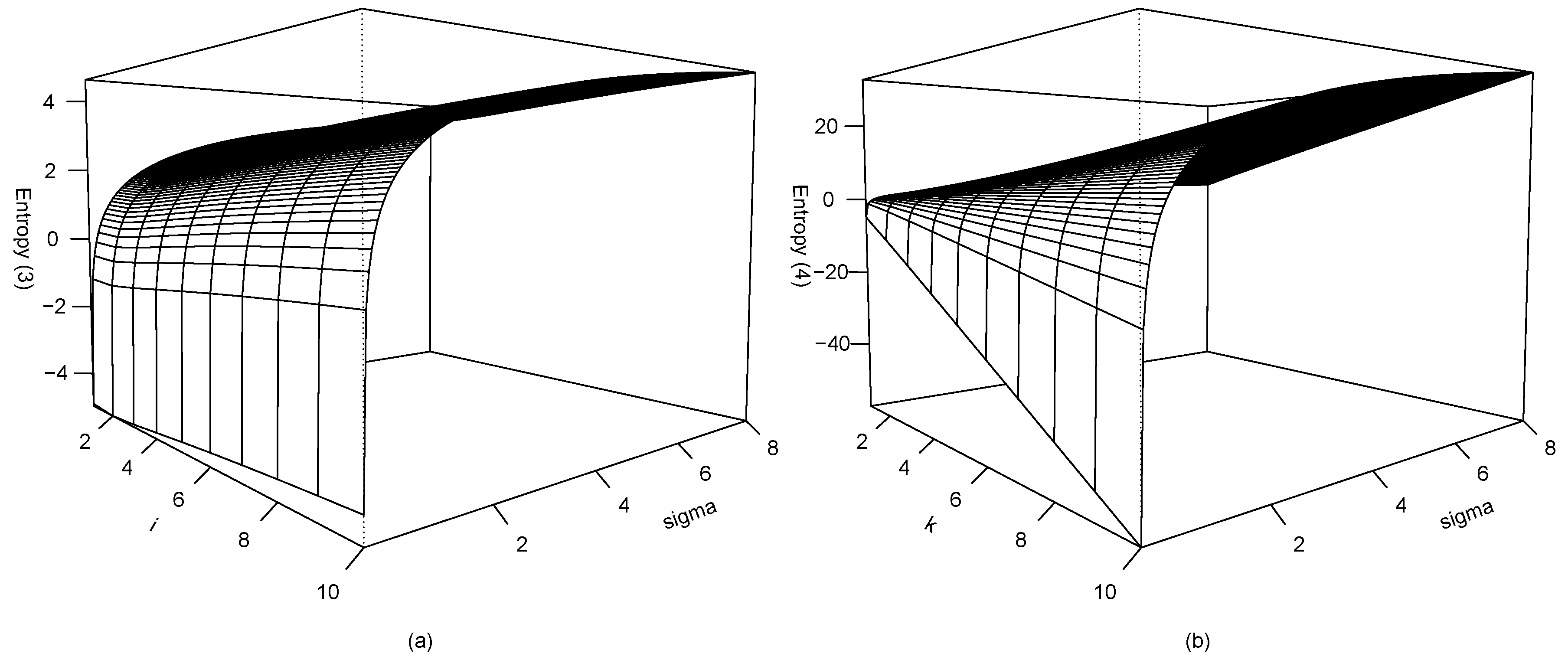
2.1. Entropy
2.2. Posterior Analysis Based on Objective Priors
3. Application
4. Conclusions
Acknowledgments
Author Contributions
Conflicts of Interest
References
- Shannon, C.E. A mathematical theory of communication. Bell Syst. Tech. J. 1948, 27, 379–423. [Google Scholar] [CrossRef]
- Baratpour, S.; Ahmadi, J.; Arghami, N.R. Entropy properties of record statistics. Stat. Pap. 2007, 48, 197–213. [Google Scholar] [CrossRef]
- Abo-Eleneen, Z.A. The entropy of progressively censored samples. Entropy 2011, 13, 437–449. [Google Scholar] [CrossRef]
- Kang, S.B.; Cho, Y.S.; Han, J.T.; Kim, J. An estimation of the entropy for a double exponential distribution based on multiply Type-II censored samples. Entropy 2012, 14, 161–173. [Google Scholar] [CrossRef]
- Seo, J.I.; Kang, S.B. Entropy estimation of generalized half-logistic distribution (GHLD) based on Type-II censored samples. Entropy 2014, 16, 443–454. [Google Scholar] [CrossRef]
- Park, S. Testing exponentiality based on the Kullback-Leibler information with the Type-II censored data. IEEE Trans. Reliab. 2005, 54, 22–26. [Google Scholar] [CrossRef]
- Rad, A.H.; Yousefzadeh, F.; Amini, M.; Arghami, N.R. Testing exponentiality based on record values. J. Iran. Stat. Soc. 2007, 6, 77–87. [Google Scholar]
- Asgharzadeh, A.; Valiollahi, R.; Abdi, M. Point and interval estimation for the logistic distribution based on record data. Stat. Oper. Res. Trans. 2016, 40, 1–24. [Google Scholar]
- Bernardo, J.M. Reference posterior distributions for Bayesian inference (with discussion). J. R. Stat. Soc. Ser. B 1979, 41, 113–147. [Google Scholar]
- Berger, J.O.; Bernardo, J.M. Estimating a product of means: Bayesian analysis with reference priors. J. Am. Stat. Assoc. 1989, 84, 200–207. [Google Scholar] [CrossRef]
- Berger, J.O.; Bernardo, J.M. On the development of reference priors (with discussion). In Bayesian Statistics IV; Bernardo, J.M., Berger, J.O., Dawid, A.P., Smith, A.F.M., Eds.; Oxford University Press: Oxford, UK, 1992; pp. 35–60. [Google Scholar]
- Devroye, L. A simple algorithm for generating random variates with a log-concave density. Computing 1984, 33, 247–257. [Google Scholar] [CrossRef]
- Roberts, G.O.; Rosenthal, J.S. Optimal scaling for various Metropolis-Hastings algorithms. Stat. Sci. 2001, 16, 351–367. [Google Scholar] [CrossRef]


| i | 1 | 2 | 3 | 4 | 5 | 6 | 7 | 8 | 9 | 10 | |
|---|---|---|---|---|---|---|---|---|---|---|---|
| 0.1 | −0.303 | −0.370 | −0.302 | −0.208 | −0.115 | −0.029 | 0.048 | 0.117 | 0.179 | 0.234 | |
| 0.5 | 1.307 | 1.239 | 1.307 | 1.401 | 1.494 | 1.580 | 1.657 | 1.727 | 1.788 | 1.844 | |
| 1 | 2.000 | 1.932 | 2.001 | 2.094 | 2.187 | 2.273 | 2.351 | 2.420 | 2.481 | 2.537 | |
| 2 | 2.693 | 2.625 | 2.694 | 2.787 | 2.880 | 2.966 | 3.044 | 3.113 | 3.175 | 3.230 | |
| 4 | 3.386 | 3.319 | 3.387 | 3.480 | 3.574 | 3.660 | 3.737 | 3.806 | 3.868 | 3.923 | |
| 8 | 4.079 | 4.012 | 4.080 | 4.174 | 4.267 | 4.353 | 4.430 | 4.499 | 4.561 | 4.616 | |
| k | 1 | 2 | 3 | 4 | 5 | 6 | 7 | 8 | 9 | 10 | |
|---|---|---|---|---|---|---|---|---|---|---|---|
| 0.1 | −0.303 | −1.250 | −2.400 | −3.632 | −4.900 | −6.187 | −7.481 | −8.780 | −10.080 | −11.382 | |
| 0.5 | 1.307 | 1.969 | 2.429 | 2.806 | 3.147 | 3.470 | 3.785 | 4.096 | 4.405 | 4.712 | |
| 1 | 2.000 | 3.355 | 4.508 | 5.579 | 6.612 | 7.629 | 8.637 | 9.641 | 10.643 | 11.644 | |
| 2 | 2.693 | 4.741 | 6.587 | 8.351 | 10.078 | 11.788 | 13.489 | 15.186 | 16.881 | 18.575 | |
| 4 | 3.386 | 6.128 | 8.667 | 11.124 | 13.544 | 15.947 | 18.341 | 20.731 | 23.120 | 25.507 | |
| 8 | 4.079 | 7.514 | 10.746 | 13.896 | 17.010 | 20.106 | 23.193 | 26.276 | 29.358 | 32.438 | |
| Estimate | 3.225 | 3.196 | 3.209 | 1.234 | 1.010 | 1.096 |
| HPD CrI | (2.137, 4.465) | (2.694, 3.904) | (2.392, 4.122) | (0.652, 2.287) | (0.386, 1.635) | (0.403, 1.935) |
| AR | 0.389 | 0.438 | 0.439 |
| Mean | Std | ||||||
|---|---|---|---|---|---|---|---|
| 3.224 | 5.262 | 6.726 | 8.089 | 9.353 | 6.531 | 2.522 | |
| 3.195 | 4.846 | 6.046 | 7.176 | 8.204 | 5.894 | 2.064 | |
| 3.221 | 5.000 | 6.288 | 7.506 | 8.629 | 6.129 | 2.226 |
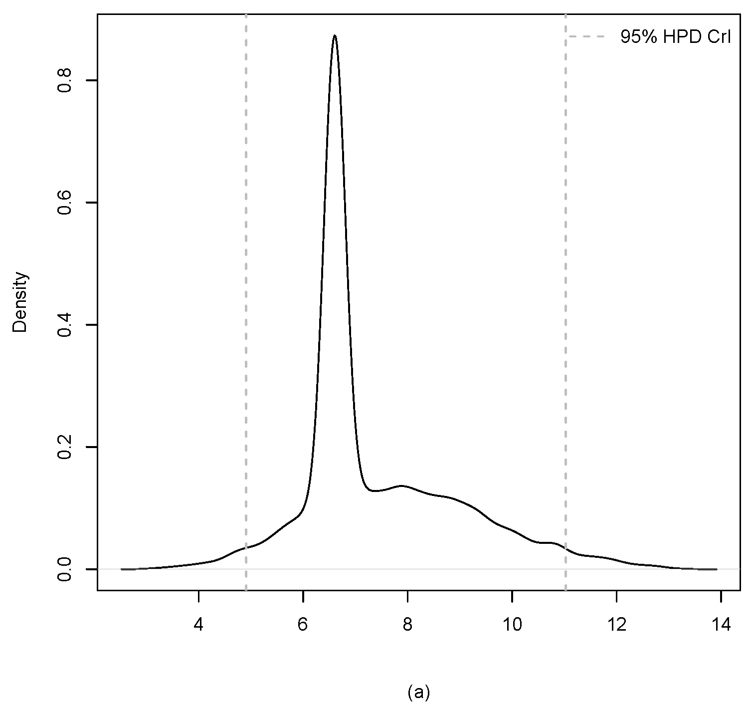
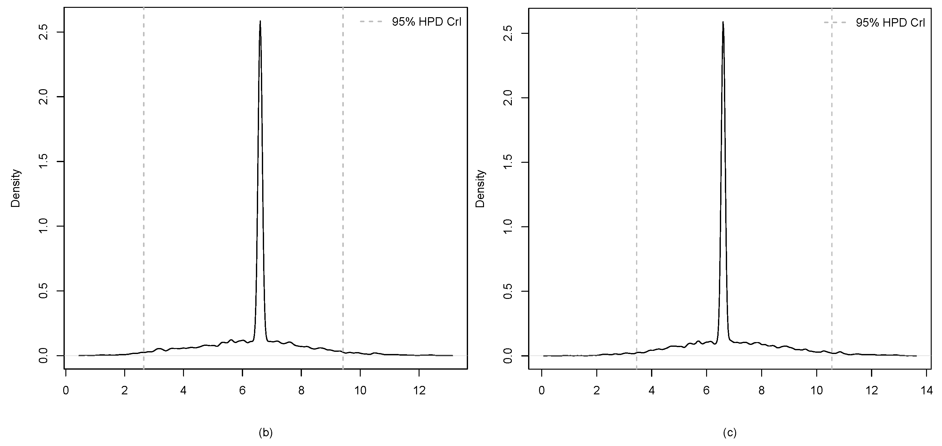
| Estimate | 7.407 | 6.431 | 6.803 |
| HPD CrI | (4.910, 11.027) | (2.648, 9.417) | (3.455, 10.557) |
© 2017 by the authors. Licensee MDPI, Basel, Switzerland. This article is an open access article distributed under the terms and conditions of the Creative Commons Attribution (CC BY) license (http://creativecommons.org/licenses/by/4.0/).
Share and Cite
Seo, J.I.; Kim, Y. Objective Bayesian Entropy Inference for Two-Parameter Logistic Distribution Using Upper Record Values. Entropy 2017, 19, 208. https://doi.org/10.3390/e19050208
Seo JI, Kim Y. Objective Bayesian Entropy Inference for Two-Parameter Logistic Distribution Using Upper Record Values. Entropy. 2017; 19(5):208. https://doi.org/10.3390/e19050208
Chicago/Turabian StyleSeo, Jung In, and Yongku Kim. 2017. "Objective Bayesian Entropy Inference for Two-Parameter Logistic Distribution Using Upper Record Values" Entropy 19, no. 5: 208. https://doi.org/10.3390/e19050208
APA StyleSeo, J. I., & Kim, Y. (2017). Objective Bayesian Entropy Inference for Two-Parameter Logistic Distribution Using Upper Record Values. Entropy, 19(5), 208. https://doi.org/10.3390/e19050208