On Linear Coding over Finite Rings and Applications to Computing

Abstract

This paper presents a coding theorem for linear coding over finite rings, in the setting of the Slepian–Wolf source coding problem. This theorem covers corresponding achievability theorems of Elias (IRE Conv. Rec. 1955, 3, 37–46) and Csiszár (IEEE Trans. Inf. Theory 1982, 28, 585–592) for linear coding over finite fields as special cases. In addition, it is shown that, for any set of finite correlated discrete memoryless sources, there always exists a sequence of linear encoders over some finite non-field rings which achieves the data compression limit, the Slepian–Wolf region. Hence, the optimality problem regarding linear coding over finite non-field rings for data compression is closed with positive confirmation with respect to existence. For application, we address the problem of source coding for computing, where the decoder is interested in recovering a discrete function of the data generated and independently encoded by several correlated i.i.d. random sources. We propose linear coding over finite rings as an alternative solution to this problem. Results in Körner–Marton (IEEE Trans. Inf. Theory 1979, 25, 219–221) and Ahlswede–Han (IEEE Trans. Inf. Theory 1983, 29, 396–411, Theorem 10) are generalized to cases for encoding (pseudo) nomographic functions (over rings). Since a discrete function with a finite domain always admits a nomographic presentation, we conclude that both generalizations universally apply for encoding all discrete functions of finite domains. Based on these, we demonstrate that linear coding over finite rings strictly outperforms its field counterpart in terms of achieving better coding rates and reducing the required alphabet sizes of the encoders for encoding infinitely many discrete functions.

1. Introduction

The problem of source coding for computing considers the scenario where a decoder is interested in recovering a function of the message(s), other than the original message(s), that is (are) i.i.d. generated and independently encoded by the source(s). In rigorous terms:

Problem 1 (Source Coding for Computing).

Given $\mathcal{S}=\{1,2,\cdots ,s\}$ and $(X_1,X_2,\cdots ,X_s)\sim p$. For each $i\in \mathcal{S}$ consider a discrete memoryless source that randomly generates i.i.d. discrete data $X_i^{\left(1\right)},X_i^{\left(2\right)},\cdots ,X_i^{\left(n\right)},\cdots$, where $X_i^{\left(n\right)}$ has a finite sample space ${\mathcal{X}}_i$ and $\left(X_1^{\left(n\right)},X_2^{\left(n\right)},\cdots ,X_s^{\left(n\right)}\right)\sim p,$ $\forall n\in {\mathbb{N}}^{+}$. For a discrete function $g:{\prod }_{i\in \mathcal{S}}{\mathcal{X}}_i\to \Omega ,$ what is the largest region $\mathcal{R}\left[g\right]\subset {\mathbb{R}}^s$, such that, $\forall (R_1,R_2,\cdots ,R_s)\in \mathcal{R}\left[g\right]$ and $\forall ϵ>0$, there exists an $N_0\in {\mathbb{N}}^{+}$, such that for all $n>N_0$, there exist s encoders ${\varphi }_i:{\mathcal{X}}_i^n\to \left[1,2^{n{R}_i}\right],i\in \mathcal{S},$ and one decoder $\psi :{\prod }_{i\in \mathcal{S}}\left[1,2^{n{R}_i}\right]\to {\Omega }^n,$ with

$$\begin{array}{c}\hfill Pr\left\{\overrightarrow{g}\left(X_1^n,\cdots ,X_s^n\right)\ne \psi \left[{\varphi }_1\left(X_1^n\right),\cdots ,{\varphi }_s\left(X_s^n\right)\right]\right\}<ϵ,\end{array}$$

(1)

where $X_i^n=\left(X_i^{\left(1\right)},X_i^{\left(2\right)},\cdots ,X_i^{\left(n\right)}\right)$ and

$$\begin{array}{c}\hfill \overrightarrow{g}\left(X_1^n,\cdots ,X_s^n\right)=\left[\begin{array}{c}g\left(X_1^{\left(1\right)},\cdots ,X_s^{\left(1\right)}\right)\\ ⋮\\ g\left(X_1^{\left(n\right)},\cdots ,X_s^{\left(n\right)}\right)\end{array}\right]\in {\Omega }^n?\end{array}$$

(2)

The region $\mathcal{R}\left[g\right]$ is called the achievable coding rate region for computing g. A rate tuple $\mathbf{R}\in {\mathbb{R}}^s$ is said to be achievable for computing g (or simply achievable) if and only if $\mathbf{R}\in \mathcal{R}\left[g\right]$. A region $\mathcal{R}\subset {\mathbb{R}}^s$ is said to be achievable for computing g (or simply achievable) if and only if $\mathcal{R}\subseteq \mathcal{R}\left[g\right]$.

If g is an identity function, the computing problem, Problem 1, is known as the Slepian–Wolf (SW) source coding problem. $\mathcal{R}\left[g\right]$ is then the SW region [1],

$$\begin{array}{c}\hfill \mathcal{R}[X_1,X_2,\cdots ,X_s]=\left.\{(R_1,R_2,\cdots ,R_s)\in {\mathbb{R}}^s\right|\sum _{j\in T}{R}_j>H\left(X_T\right|X_{T^c}),\forall \varnothing \ne T\subseteq \mathcal{S}\},\end{array}$$

(3)

where $T^c$ is the complement of T in $\mathcal{S}$ and $X_T\left(X_{T^c}\right)$ is the random variable array ${\prod }_{j\in T}{X}_j\left({\prod }_{j\in T^c}{X}_j\right)$. However, from [1] it is hard to draw conclusions regarding the structure (linear or not) of the encoders, as the corresponding mappings are chosen randomly among all feasible mappings. This limits the scope of their potential applications. As a consequence, linear coding over finite fields (LCoF), namely ${\mathcal{X}}_i$’s are injectively mapped into some subsets of some finite fields and the ${\varphi }_i$’s are chosen as linear mappings over these fields, is considered. It is shown that LCoF achieves the same encoding limit, the SW region [2,3]. Although it seems straightforward to study linear mappings over rings (non-field rings in particular), it has not been proved (nor denied) that linear encoding over non-field rings can be equally optimal.

For an arbitrary discrete function g, Problem 1 remains open in general, and $\mathcal{R}[X_1,X_2,\cdots ,X_s]\subseteq \mathcal{R}\left[g\right]$ obviously. Making use of Elias’ theorem on binary linear codes [2], Körner–Marton [4] shows that $\mathcal{R}\left[{\oplus }_2\right]$ (“${\oplus }_2$” is the modulo-two sum) contains the region

$$\begin{array}{c}\hfill \tilde{\mathcal{R}}=\left\{(R_1,R_2)\in {\mathbb{R}}^2|R_1,R_2>H\left(X_1{\oplus }_2{X}_2\right)\right\}.\end{array}$$

(4)

This region is not contained in the SW region for certain distributions. In other words, $\mathcal{R}\left[{\oplus }_2\right]⊋\mathcal{R}[X_1,X_2]$. Combining the standard random coding technique and Elias’ result, [5] shows that $\mathcal{R}\left[{\oplus }_2\right]$ can be strictly larger than the convex hull of the union $\mathcal{R}[X_1,X_2]\cup \tilde{\mathcal{R}}$. However, the functions considered in these works are relatively simple. With a polynomial approach, [6,7] generalize the result of Ahlswede–Han ([5], Theorem 10) to the scenario of g being arbitrary. Making use of the fact that a discrete function is essentially a polynomial function (see Definition 2) over some finite field, an achievable region is given for computing an arbitrary discrete function. Such a region contains and can be strictly larger (depending on the precise function and distribution under consideration) than the SW region. Conditions under which $\mathcal{R}\left[g\right]$ is strictly larger than the SW region are presented in [6,8] from different perspectives, respectively. The cases regarding Abelian group codes are covered in [9,10,11].

The present work proposes replacing the linear encoders over finite fields from Elias [2] and Csiszár [3] with linear encoders over finite rings in the case of the problems accounted for above. Achievability theorems related to linear coding over finite rings (LCoR) for SW data compression are presented, covering the results in [2,3] as special cases in the sense of characterizing the achievable region. In addition, it is proved that there always exists a sequence of linear encoders over some finite non-field rings that achieves the SW region for any scenario of SW. Therefore, the issue of optimality of linear coding over finite non-field rings for data compression is closed with respect to existence. Furthermore, we also consider LCoR as an alternative technique for the general computing problem, Problem 1. Results from Körner–Marton [4], Ahlswede–Han ([5], Theorem 10) and [7] are generalized to corresponding ring versions for encoding (pseudo) nomographic functions (over rings). Since any discrete function with a finite domain admits a nomographic presentation, we conclude that our results universally apply for encoding all discrete functions of finite domains. Finally, it is shown that our ring approach dominates its field counterpart in terms of achieving better coding rates and reducing alphabet sizes of the encoders for encoding some discrete function. The proof is done by taking advantage of the fact that the characteristic of a ring can be any positive integer while the characteristic of a field must be a prime. From this observation used in the proof, it is seen that there are actually infinite many such functions.

2. Rings, Ideals and Linear Mappings

We start by introducing some fundamental algebraic concepts and related properties. Readers who are already familiar with this material may still choose to go through quickly to identify our notation.

Definition 1.

The tuple $[\mathfrak{R},+,·]$ is called a ring if the following criteria are met:

1. 

$[\mathfrak{R},+]$ is an Abelian group ;

2. 

There exists a multiplicative identity $1\in \mathfrak{R}$, namely, $1·a=a·1=a$, $\forall a\in \mathfrak{R}$;

3. 

$\forall a,b,c\in \mathfrak{R}$, $a·b\in \mathfrak{R}$ and $(a·b)·c=a·(b·c)$;

4. 

$\forall a,b,c\in \mathfrak{R}$, $a·(b+c)=(a·b)+(a·c)$ and $(b+c)·a=(b·a)+(c·a)$.

We often write $\mathfrak{R}$ for $[\mathfrak{R},+,·]$ when the operations considered are known from the context. The operation “·” is usually written by juxtaposition, $ab$ for $a·b$, for all $a,b\in \mathfrak{R}$.

A ring $[\mathfrak{R},+,·]$ is said to be commutative if $\forall a,b\in \mathfrak{R}$, $a·b=b·a$. In Definition 1, the identity of the group $[\mathfrak{R},+]$, denoted by 0, is called the zero. A ring $[\mathfrak{R},+,·]$ is said to be finite if the cardinality $\left|\mathfrak{R}\right|$ is finite, and $\left|\mathfrak{R}\right|$ is called the order of $\mathfrak{R}$. The set ${\mathbb{Z}}_q$ of integers modulo q is a commutative finite ring with respect to the modular arithmetic. For any ring $\mathfrak{R}$, the set of all polynomials of s indeterminants over $\mathfrak{R}$ is an infinite ring.

Definition 2.

A polynomial function (Polynomial and polynomial function are distinct concepts.) of k variables over a finite ring $\mathfrak{R}$ is a function $g:{\mathfrak{R}}^k\to \mathfrak{R}$ of the form

$$\begin{array}{c}\hfill g(x_1,x_2,\cdots ,x_k)=\sum _{j=0}^m{a}_j{x}_1^{m_{1j}}{x}_2^{m_{2j}}\cdots x_k^{m_{kj}},\end{array}$$

(5)

where $a_j\in \mathfrak{R}$ and m and $m_{ij}$’s are non-negative integers. The set of all the polynomial functions of k variables over ring $\mathfrak{R}$ is designated by $\mathfrak{R}\left[k\right]$.

Remark 1.

Polynomial and polynomial function are sometimes only defined over a commutative ring [12,13]. It is a very delicate matter to define them over a non-commutative ring [14,15], due to the fact that $x_1{x}_2$ and $x_2{x}_1$ can become different objects. We choose to define “polynomial functions” with Formula (5) because those functions are within the scope of this paper’s interest.

Proposition 1.

Given s rings ${\mathfrak{R}}_1,{\mathfrak{R}}_2,\cdots ,{\mathfrak{R}}_s$, for any non-empty set $T\subseteq \{1,2,\cdots ,s\}$, the Cartesian product (see [12]) ${\mathfrak{R}}_T={\prod }_{i\in T}{\mathfrak{R}}_i$ forms a new ring $[{\mathfrak{R}}_T,+,·]$ with respect to the component-wise operations defined as follows:

$$\begin{array}{cc}\hfill {\mathbf{a}}^{\prime }+{\mathbf{a}}^{″}=& \left(a_1^{\prime }+a_1^{″},a_2^{\prime }+a_2^{″},\cdots ,a_{\left|T\right|}^{\prime }+a_{\left|T\right|}^{″}\right),\hfill \end{array}$$

(6)

$$\begin{array}{cc}\hfill {\mathbf{a}}^{\prime }·{\mathbf{a}}^{″}=& \left(a_1^{\prime }{a}_1^{″},a_2^{\prime }{a}_2^{″},\cdots ,a_{\left|T\right|}^{\prime }{a}_{\left|T\right|}^{″}\right),\hfill \end{array}$$

(7)

$\forall {\mathbf{a}}^{\prime }=\left(a_1^{\prime },a_2^{\prime },\cdots ,a_{\left|T\right|}^{\prime }\right),{\mathbf{a}}^{″}=\left(a_1^{″},a_2^{″},\cdots ,a_{\left|T\right|}^{″}\right)\in {\mathfrak{R}}_T$.

Remark 2.

In Proposition 1, $[{\mathfrak{R}}_T,+,·]$ is called the direct product of $\left\{{\mathfrak{R}}_i\right|i\in T\}$. It can be easily seen that $(0,0,\cdots ,0)$ and $(1,1,\cdots ,1)$ are the zero and the multiplicative identity of $[{\mathfrak{R}}_T,+,·]$, respectively.

Definition 3.

A non-zero element a of a ring $\mathfrak{R}$ is said to be invertible , if and only if there exists $b\in \mathfrak{R}$, such that $ab=ba=1$. b is called the inverse of a, denoted by $a^{-1}$. An invertible element of a ring is called a unit.

Remark 3.

It can be proved that the inverse of a unit is unique. By definition, the multiplicative identity is the inverse of itself.

Let ${\mathfrak{R}}^{*}=\mathfrak{R}\backslash \left\{0\right\}$. The ring $[\mathfrak{R},+,·]$ is a field if and only if $[{\mathfrak{R}}^{*},·]$ is an Abelian group. In other words, all non-zero elements of $\mathfrak{R}$ are invertible. All fields are commutative rings. ${\mathbb{Z}}_q$ is a field if and only if q is a prime. All finite fields of the same order are isomorphic to each other ([16], p. 549). This “unique” field of order q is denoted by ${\mathbb{F}}_q$. It is necessary that q is a power of a prime. More details regarding finite fields can be found in ([16], Chapter 14.3).

Theorem 1

(Wedderburn’s little theorem [12]). Let $\mathfrak{R}$ be a finite ring. $\mathfrak{R}$ is a field if and only if all non-zero elements of $\mathfrak{R}$ are invertible.

Remark 4.

Wedderburn’s little theorem guarantees commutativity for a finite ring if all of its non-zero elements are invertible. Hence, a finite ring is either a field or at least one of its elements has no inverse. However, a finite commutative ring is not necessary a field, e.g., ${\mathbb{Z}}_q$ is not a field if q is not a prime.

Definition 4

([16]). The characteristic of a finite ring $\mathfrak{R}$ is defined to be the smallest positive integer m, such that ${\sum }_{j=1}^{m}1=0$, where 0 and 1 are the zero and the multiplicative identity of $\mathfrak{R}$, respectively. The characteristic of $\mathfrak{R}$ is often denoted by $\mathrm{Char}\left(\mathfrak{R}\right)$.

Remark 5.

Clearly, $\mathrm{Char}\left({\mathbb{Z}}_q\right)=q$. For a finite field ${\mathbb{F}}_q$, $\mathrm{Char}\left({\mathbb{F}}_q\right)$ is always the prime $q_0$ such that $q=q_0^n$ for some integer n ([12], Proposition 2.137).

Proposition 2.

Let ${\mathbb{F}}_q$ be a finite field. For any $0\ne a\in {\mathbb{F}}_q$, $m=\mathrm{Char}\left({\mathbb{F}}_q\right)$ if and only if m is the smallest positive integer such that ${\sum }_{j=1}^{m}a=0$.

Proof. 

Since $a\ne 0$,

$$\begin{array}{c}\hfill \sum _{j=1}^{m}a=0\Rightarrow a^{-1}\sum _{j=1}^{m}a=a^{-1}·0\Rightarrow \sum _{j=1}^{m}1=0\Rightarrow \sum _{j=1}^{m}a=0\end{array}$$

(8)

The statement is proved. ☐

Definition 5.

A subset $\mathfrak{I}$ of a ring $[\mathfrak{R},+,·]$ is said to be a left ideal of $\mathfrak{R}$, denoted by $\mathfrak{I}{\le }_l\mathfrak{R}$, if and only if

1. 

$[\mathfrak{I},+]$ is a subgroup of $[\mathfrak{R},+]$;

2. 

$\forall x\in \mathfrak{I}$ and $\forall a\in \mathfrak{R}$, $a·x\in \mathfrak{I}$.

If condition 2 is replaced by

3. 

$\forall x\in \mathfrak{I}$ and $\forall a\in \mathfrak{R}$, $x·a\in \mathfrak{I}$,

then $\mathfrak{I}$ is called a right ideal of $\mathfrak{R}$, denoted by $\mathfrak{I}{\le }_r\mathfrak{R}$. $\left\{0\right\}$ is a trivial left (right) ideal, usually denoted by 0.

The cardinality $\left|\mathfrak{I}\right|$ is called the order of a finite left (right) ideal $\mathfrak{I}$.

Remark 6.

Let $\left\{a_1,a_2,\cdots ,a_n\right\}$ be a non-empty set of elements of some ring $\mathfrak{R}$. It is easy to verify that ${\langle a_1,a_2,\cdots ,a_n\rangle }_r=\left\{{\sum }_{i=1}^n{a}_i{b}_i\right|b_i\in \mathfrak{R},\forall 1\le i\le n\}$ is a right ideal and ${\langle a_1,a_2,\cdots ,a_n\rangle }_l=\left\{{\sum }_{i=1}^n{b}_i{a}_i\right|b_i\in \mathfrak{R},\forall 1\le i\le n\}$ is a left ideal. Furthermore, ${\langle a_1,a_2,\cdots ,a_n\rangle }_r=\mathfrak{R}$ and ${\langle a_1,a_2,\cdots ,a_n\rangle }_l=\mathfrak{R}$ if $a_i$ is a unit for some $1\le i\le n$.

It is well-known that if $\mathfrak{I}{\le }_l\mathfrak{R}$, then $\mathfrak{R}$ is divided into disjoint cosets which are of equal size (cardinality). For any coset $\mathfrak{J}$, $\mathfrak{J}=x+\mathfrak{I}=\left\{x+y|y\in \mathfrak{I}\right\}$, $\forall x\in \mathfrak{J}$. The set of all cosets forms a left module over $\mathfrak{R}$, denoted by $\mathfrak{R}/\mathfrak{I}$. Similarly, $\mathfrak{R}/\mathfrak{I}$ becomes a right module over $\mathfrak{R}$ if $\mathfrak{I}{\le }_r\mathfrak{R}$ [17]. Of course, $\mathfrak{R}/\mathfrak{I}$ can also be considered as a quotient group [12]. However, its structure is well richer than simply being a quotient group.

Proposition 3.

Let ${\mathfrak{R}}_i$ ($1\le i\le s$) be a ring and $\mathfrak{R}={\prod }_{i=1}^s{\mathfrak{R}}_i$. For any $\mathfrak{A}\subseteq \mathfrak{R}$, $\mathfrak{A}{\le }_l\mathfrak{R}$ (or $\mathfrak{A}{\le }_r\mathfrak{R}$) if and only if $\mathfrak{A}={\prod }_{i=1}^s{\mathfrak{A}}_i$ and ${\mathfrak{A}}_i{\le }_l{\mathfrak{R}}_i$ (or ${\mathfrak{A}}_i{\le }_r{\mathfrak{R}}_i$), $\forall 1\le i\le s$.

Proof. 

We prove for the ${\le }_l$ case only, and the ${\le }_r$ case follows from a similar argument. Let ${\pi }_i$ ($1\le i\le s$) be the coordinate function assigning every element in $\mathfrak{R}$ its ith component. Then $\mathfrak{A}\subseteq {\prod }_{i=1}^s{\mathfrak{A}}_i$, where ${\mathfrak{A}}_i={\pi }_i\left(\mathfrak{A}\right)$. Moreover, for any

$$\begin{array}{c}\hfill \mathbf{x}=({\pi }_1\left({\mathbf{x}}_1\right),{\pi }_2\left({\mathbf{x}}_2\right),\cdots ,{\pi }_s\left({\mathbf{x}}_s\right))\in \prod _{i=1}^s{\mathfrak{A}}_i,\end{array}$$

(9)

where ${\mathbf{x}}_i\in \mathfrak{A}$ for all feasible i, we have that

$$\begin{array}{c}\hfill \mathbf{x}=\sum _{i=1}^s{\mathbf{e}}_i{\mathbf{x}}_i,\end{array}$$

(10)

where ${\mathbf{e}}_i\in \mathfrak{R}$ has the ith coordinate being 1 and others being 0. If $\mathfrak{A}{\le }_l\mathfrak{R}$, then $\mathbf{x}\in \mathfrak{A}$ by definition. Therefore, ${\prod }_{i=1}^s{\mathfrak{A}}_i\subseteq \mathfrak{A}$. Consequently, $\mathfrak{A}={\prod }_{i=1}^s{\mathfrak{A}}_i$. Since ${\pi }_i$ is a homomorphism, we also have that ${\mathfrak{A}}_i{\le }_l{\mathfrak{R}}_i$ for all feasible i. The other direction is easily verified by definition. ☐

Remark 7.

It is worthwhile to point out that Proposition 3 does not hold for infinite index set, namely, $\mathfrak{R}={\prod }_{i\in I}{\mathfrak{R}}_i$, where I is not finite.

For any $\varnothing \ne T\subseteq \mathcal{S}$, Proposition 3 states that any left (right) ideal of ${\mathfrak{R}}_T$ is a Cartesian product of some left (right) ideals of ${\mathfrak{R}}_i$, $i\in T$. Let ${\mathfrak{I}}_i$ be a left (right) ideal of ring ${\mathfrak{R}}_i$ ($1\le i\le s$). We define ${\mathfrak{I}}_T$ to be the left (right) ideal ${\prod }_{i\in T}{\mathfrak{I}}_i$ of ${\mathfrak{R}}_T$.

Let ${\mathbf{x}}^t$ be the transpose of a vector (or matrix) $\mathbf{x}$.

Definition 6.

A mapping $f:{\mathfrak{R}}^n\to {\mathfrak{R}}^m$ given as:

$$\begin{array}{c}\hfill f(x_1,x_2,\cdots ,x_n)={\left(\sum _{j=1}^n{a}_{1,j}{x}_j,\cdots ,\sum _{j=1}^n{a}_{m,j}{x}_j\right)}^t,\forall (x_1,x_2,\cdots ,x_n)\in {\mathfrak{R}}^n,\end{array}$$

(11)

where t stands for transposition and $a_{i,j}\in \mathfrak{R}$ for all feasible i and j, is called a left linear mapping over ring $\mathfrak{R}$. Similarly,

$$\begin{array}{c}\hfill f(x_1,x_2,\cdots ,x_n)={\left(\sum _{j=1}^n{x}_j{a}_{1,j},\cdots ,\sum _{j=1}^n{x}_j{a}_{m,j}\right)}^t,\forall (x_1,x_2,\cdots ,x_n)\in {\mathfrak{R}}^n,\end{array}$$

(12)

defines a right linear mapping over ring $\mathfrak{R}$. If $m=1$, then f is called a left ( right ) linear function over $\mathfrak{R}$.

From now on, left linear mapping (function) or right linear mapping (function) are simply called linear mapping (function). This will not lead to any confusion since the intended use can usually be clearly distinguished from the context.

Remark 8.

The mapping f in Definition 6 is called linear in accordance with the definition of linear mapping (function) over a field. In fact, the two structures have several similar properties. Moreover, (11) is equivalent to

$$\begin{array}{c}\hfill f(x_1,x_2,\cdots ,x_n)=\mathbf{A}{\left(x_1,x_2,\cdots ,x_n\right)}^t,\forall (x_1,x_2,\cdots ,x_n)\in {\mathfrak{R}}^n,\end{array}$$

(13)

where $\mathbf{A}$ is an $m\times n$ matrix over $\mathfrak{R}$ and ${\left[\mathbf{A}\right]}_{i,j}=a_{i,j}$ for all feasible i and j. $\mathbf{A}$ is named the coefficient matrix. It is easy to prove that a linear mapping is uniquely determined by its coefficient matrix, and vice versa. The linear mapping f is said to be trivial , denoted by 0, if $\mathbf{A}$ is the zero matrix , i.e., ${\left[\mathbf{A}\right]}_{i,j}=0$ for all feasible i and j.

It should be noted that an interesting approach to coding over an Abelian group was presented in [9,10,11]. However, we emphasize that even if group, field and ring are closely related algebraic structures, the definition of the group encoder in [11] and the linear encoder in [3] and in the present work are in general fundamentally different (although there is an overlap in special cases). To highlight in more detail the difference between linear encoding (this work and [3]) and encoding over a group, as in [11], which is a nonlinear operation in general, take the Abelian group $G={\mathbb{Z}}_2\oplus {\mathbb{Z}}_2$, the field ${\mathbb{F}}_4$ of order 4 and the matrix ring ${\mathbb{M}}_{L,2}=\left\{\left.\left[\begin{array}{cc}a& 0\\ b& a\end{array}\right]\right|a,b\in {\mathbb{Z}}_2\right\}$ as examples.

• By ([11], Example 2), the Abelian group encoder encodes the source $\widehat{Z}=(X,Y)\in G$ based on a Slepian–Wolf like scheme. Namely, two binary linear encoders encode $X^n$ and $Y^n$ separately as two binary sources. Therefore, the lengths of the codewords from encoding $X^n$ and $Y^n$ can even be different, and the encoder is in general a highly nonlinear device.
• On the other hand, the linear encoder over either ${\mathbb{F}}_4$ or ${\mathbb{M}}_{L,2}$ simply outputs a linear combination of the vector ${\widehat{Z}}^n$, namely $\mathbf{A}{\widehat{Z}}^n$ for some matrix $\mathbf{A}$ over ${\mathbb{F}}_4$ or ${\mathbb{M}}_{L,2}$.
• However, if one requires that the codewords from encoding $X^n$ and $Y^n$ be of the same length in (1), then the output from encoding ${\widehat{Z}}^n$ is the same as $\tilde{\mathbf{A}}{\widehat{Z}}^n$ for some matrix $\tilde{\mathbf{A}}$ over ring ${\mathbb{Z}}_2\times {\mathbb{Z}}_2$ (a specific product ring whose multiplication is significantly different from those of ${\mathbb{F}}_4$ or ${\mathbb{M}}_{L,2}$). In other words, in this quite specific special case, the encoder becomes linear over a product ring of modulo integers, which is a sub-class of the completely general ring structures considered in this paper.

We also note that in some source network problems, linear codes appear superior to others [3]. For instance, for encoding the modulo-two sum of binary symmetric sources, linear coding over ${\mathbb{F}}_4$ or ${\mathbb{M}}_{L,2}$ achieves the optimal Körner–Marton region [4] (the ${\mathbb{M}}_{L,2}$ case will be established in later sections), while coding over G achieves the sub-optimal Slepian–Wolf region ([11], p. 1509). To avoid any remaining confusion, we in Appendix D present additional details regarding the differences between linear coding, as in the present work and in [3], and coding over an Abelian group, as in [11].

Let $\mathbf{A}$ be an $m\times n$ matrix over ring $\mathfrak{R}$ and $f\left(\mathbf{x}\right)=\mathbf{A}\mathbf{x}$, $\forall \mathbf{x}\in {\mathfrak{R}}^n$. For the system of linear equations

$$\begin{array}{c}\hfill f\left(\mathbf{x}\right)=\mathbf{A}\mathbf{x}=0,\mathrm{where}0={(0,0,\cdots ,0)}^t\in {\mathfrak{R}}^m,\end{array}$$

(14)

let $\mathfrak{S}\left(f\right)$ be the set of all solutions, namely $\mathfrak{S}\left(f\right)=\left\{\mathbf{x}\in {\mathfrak{R}}^n|f\left(\mathbf{x}\right)=0\right\}$. It is obvious that $\mathfrak{S}\left(f\right)={\mathfrak{R}}^n$ if f is trivial, i.e., $\mathbf{A}$ is the zero matrix. If $\mathfrak{R}$ is a field, then $\mathfrak{S}\left(f\right)$ is a subspace of ${\mathfrak{R}}^n$. We conclude this section with a lemma regarding the cardinalities of ${\mathfrak{R}}^n$ and $\mathfrak{S}\left(f\right)$ in the following.

Lemma 1.

For a finite ring $\mathfrak{R}$ and a linear function

$$\begin{array}{cc}\hfill f:& \mathbf{x}\mapsto (a_1,a_2,\cdots ,a_n)\mathbf{x}\hfill \end{array}$$

(15)

$$\begin{array}{cc}\hfill (f:& \mathbf{x}\mapsto {\mathbf{x}}^t{(a_1,a_2,\cdots ,a_n)}^t),\forall \mathbf{x}\in {\mathfrak{R}}^n,\hfill \end{array}$$

(16)

we have

$$\begin{array}{c}\hfill {\displaystyle \frac{\left|\mathfrak{S}\left(f\right)\right|}{{\left|\mathfrak{R}\right|}^n}}={\displaystyle \frac{1}{\left|\mathfrak{I}\right|}},\end{array}$$

(17)

where $\mathfrak{I}={\langle a_1,a_2,\cdots ,a_n\rangle }_r$ $\left(\mathfrak{I}={\langle a_1,a_2,\cdots ,a_n\rangle }_l\right)$. In particular, if $a_i$ is invertible for some $1\le i\le n$, then $\left|\mathfrak{S}\left(f\right)\right|={\left|\mathfrak{R}\right|}^{n-1}$.

Proof. 

It is obvious that the image $f\left({\mathfrak{R}}^n\right)=\mathfrak{I}$ by definition. Moreover, $\forall x\ne y\in \mathfrak{I}$, the pre-images $f^{-1}\left(x\right)$ $f^{-1}\left(y\right)$ satisfy $f^{-1}\left(x\right)\cap f^{-1}\left(y\right)=\varnothing$ and $\left|f^{-1}\left(x\right)\right|=\left|f^{-1}\left(y\right)\right|=\left|\mathfrak{S}\left(f\right)\right|$. Therefore, $\left|\mathfrak{I}\right|\left|\mathfrak{S}\left(f\right)\right|={\left|\mathfrak{R}\right|}^n$, i.e., ${\displaystyle \frac{\left|\mathfrak{S}\left(f\right)\right|}{{\left|\mathfrak{R}\right|}^n}}={\displaystyle \frac{1}{\left|\mathfrak{I}\right|}}$. Moreover, if $a_i$ is a unit, then $\mathfrak{I}=\mathfrak{R}$, thus, $\left|\mathfrak{S}\left(f\right)\right|={\left|\mathfrak{R}\right|}^n/\left|\mathfrak{R}\right|={\left|\mathfrak{R}\right|}^{n-1}$. ☐

3. Linear Coding over Finite Rings

In this section, we will present a coding rate region achieved with LCoR for the SW source coding problem, i.e., g is an identity function in Problem 1. This region is exactly the SW region if all the rings considered are fields. However, being field is not necessary as seen in Section 5, where the issue of optimality is addressed.

Before proceeding, a subtlety needs to be cleared out. It is assumed that a source generates data taking values from a finite sample space ${\mathcal{X}}_i$, while ${\mathcal{X}}_i$ does not necessarily admit any algebraic structure. We have to either assume that ${\mathcal{X}}_i$ is with a certain algebraic structure, for instance ${\mathcal{X}}_i$ is a ring, or injectively map elements of ${\mathcal{X}}_i$ into some algebraic structure. In our subsequent discussions, we assume that ${\mathcal{X}}_i$ is mapped into a finite ring ${\mathfrak{R}}_i$ of order at least $\left|{\mathcal{X}}_i\right|$ by some injection ${\mathsf{\Phi }}_i$. Hence, ${\mathcal{X}}_i$ can simply be treated as a subset ${\mathsf{\Phi }}_i\left({\mathcal{X}}_i\right)\subseteq {\mathfrak{R}}_i$ for a fixed ${\mathsf{\Phi }}_i$. When required, ${\mathsf{\Phi }}_i$ can also be selected to obtain desired outcomes.

To facilitate our discussion, the following notation is used. For $\varnothing \ne T\subseteq \mathcal{S}$, $X_T$ ($x_T$ and ${\mathcal{X}}_T$ resp.) is defined to be the Cartesian product

$$\begin{array}{c}\hfill \prod _{i\in T}{X}_i\left(\prod _{i\in T}{x}_i\mathrm{and}\prod _{i\in T}{\mathcal{X}}_i\mathrm{resp}.\right),\end{array}$$

(18)

where $x_i\in {\mathcal{X}}_i$ is a realization of $X_i$. If $\left(X_1,X_2,\cdots ,X_s\right)\sim p$, we denote the marginal of p with respect to $X_T$ by $p_{X_T}$, i.e., $X_T\sim p_{X_T}$, define the support

$$\begin{array}{cc}\hfill \mathrm{supp}\left(p_{X_T}\right)=& \left\{\left.x_T\in {\mathcal{X}}_T\right|p_{X_T}\left(x_T\right)>0\right\}\mathrm{and}\hfill \end{array}$$

(19)

$$\begin{array}{cc}\hfill H\left(p_{X_T}\right)=& H\left(X_T\right).\hfill \end{array}$$

(20)

For simplicity, $\mathcal{M}\left({\mathcal{X}}_{\mathcal{S}},{\mathfrak{R}}_{\mathcal{S}}\right)$ is defined to be

$$\begin{array}{c}\hfill \left\{\left.\left({\mathsf{\Phi }}_1,{\mathsf{\Phi }}_2,\cdots ,{\mathsf{\Phi }}_s\right)\right|{\mathsf{\Phi }}_i:{\mathcal{X}}_i\to {\mathfrak{R}}_i\mathrm{is}\mathrm{injective},\forall i\in \mathcal{S}\right\}\end{array}$$

(21)

($\left|{\mathfrak{R}}_i\right|\ge \left|{\mathcal{X}}_i\right|$ is implicitly assumed), and $\mathsf{\Phi }\left(x_T\right)={\prod }_{i\in T}{\mathsf{\Phi }}_i\left(x_i\right)$ for any $\mathsf{\Phi }\in \mathcal{M}\left({\mathcal{X}}_{\mathcal{S}},{\mathfrak{R}}_{\mathcal{S}}\right)$ and $x_T\in {\mathcal{X}}_T$. For any $\mathsf{\Phi }\in \mathcal{M}\left({\mathcal{X}}_{\mathcal{S}},{\mathfrak{R}}_{\mathcal{S}}\right)$, let

$$\begin{gathered} {\mathcal{R}}_{\mathsf{\Phi }}=\{\left(R_1,R_2,\cdots ,R_s\right)\in {\mathbb{R}}^s\left|{\sum }_{i\in T}{\displaystyle \frac{R_{i}log\left|{\mathfrak{I}}_i\right|}{log|{\mathfrak{R}}_i|}}>r\left(T,{\mathfrak{I}}_T\right),\right. \\ \forall \varnothing \ne T\subseteq \mathcal{S},\forall 0\ne {\mathfrak{I}}_i{\le }_l{\mathfrak{R}}_i\}, \end{gathered}$$

(22)

where $r\left(T,{\mathfrak{I}}_T\right)=H\left(X_T\right|X_{T^c})-H\left(Y_{{\mathfrak{R}}_T/{\mathfrak{I}}_T}\right|X_{T^c})=H\left(X_T\right|Y_{{\mathfrak{R}}_T/{\mathfrak{I}}_T},X_{T^c})$ and $Y_{{\mathfrak{R}}_T/{\mathfrak{I}}_T}=\mathsf{\Phi }\left(X_T\right)+{\mathfrak{I}}_T$ is a random variable with sample space ${\mathfrak{R}}_T/{\mathfrak{I}}_T$.

Theorem 2.

${\mathcal{R}}_{\mathsf{\Phi }}$ is achievable with linear coding over the finite rings ${\mathfrak{R}}_1,{\mathfrak{R}}_2,\cdots ,{\mathfrak{R}}_s$. In exact terms, $\forall ϵ>0$, there exists $N_0\in {\mathbb{N}}^{+}$, for all $n>N_0$, there exist linear encoders (left linear mappings to be more precise) ${\varphi }_i:\mathsf{\Phi }{\left({\mathcal{X}}_i\right)}^n\to {\mathfrak{R}}_i^{k_i}$ ($i\in \mathcal{S}$) and a decoder ψ, such that

$$\begin{array}{c}\hfill Pr\left\{\psi \left(\prod _{i\in S}{\varphi }_i\left({\mathbf{X}}_i\right)\right)\ne \prod _{i\in S}{\mathbf{X}}_i\right\}<ϵ,\end{array}$$

(23)

where ${\mathbf{X}}_i={\left(\mathsf{\Phi }\left(X_i^{\left(1\right)}\right),\mathsf{\Phi }\left(X_i^{\left(2\right)}\right),\cdots ,\mathsf{\Phi }\left(X_i^{\left(n\right)}\right)\right)}^t$, as long as

$$\begin{array}{c}\hfill \left({\displaystyle \frac{k_{1}log\left|{\mathfrak{R}}_1\right|}{n}},{\displaystyle \frac{k_{2}log\left|{\mathfrak{R}}_2\right|}{n}},\cdots ,{\displaystyle \frac{k_{s}log\left|{\mathfrak{R}}_s\right|}{n}}\right)\in {\mathcal{R}}_{\mathsf{\Phi }}.\end{array}$$

(24)

Proof. 

The proof is given in Section 4. ☐

The following is a concrete example providing some insight into this theorem.

Example 1.

Consider the single source scenario, where $X_1\sim p$ and ${\mathcal{X}}_1={\mathbb{Z}}_6$, specified as follows.

$X_1$	0	1	2	3	4	5
$p\left(X_1\right)$	$0.05$	$0.1$	$0.15$	$0.2$	$0.2$	$0.3$

Obviously, ${\mathbb{Z}}_6$ contains 3 non-trivial ideals ${\mathfrak{I}}_1=\{0,3\}$, ${\mathfrak{I}}_2=\{0,2,4\}$ and ${\mathbb{Z}}_6$, and $Y_{{\mathbb{Z}}_6/{\mathfrak{I}}_1}$ and $Y_{{\mathbb{Z}}_6/{\mathfrak{I}}_2}$ admit the distributions

respectively. In addition, $Y_{{\mathbb{Z}}_6/{\mathbb{Z}}_6}={\mathbb{Z}}_6$ is a constant. Thus, by Theorem 2, rate $R_1$ is achievable if

$$\begin{array}{cc}\hfill {\displaystyle \frac{R_{1}log\left|{\mathfrak{I}}_1\right|}{log\left|{\mathbb{Z}}_6\right|}}=& {\displaystyle \frac{R_{1}log2}{log6}}>H\left(X_1\right)-H\left(Y_{{\mathbb{Z}}_6/{\mathfrak{I}}_1}\right)=2.40869-1.53949=0.86920,\hfill \\ \hfill {\displaystyle \frac{R_{1}log\left|{\mathfrak{I}}_2\right|}{log\left|{\mathbb{Z}}_6\right|}}=& {\displaystyle \frac{R_{1}log3}{log6}}>H\left(X_1\right)-H\left(Y_{{\mathbb{Z}}_6/{\mathfrak{I}}_2}\right)=2.40869-0.97095=1.43774\hfill \\ \hfill and{\displaystyle \frac{R_{1}log\left|{\mathbb{Z}}_6\right|}{log\left|{\mathbb{Z}}_6\right|}}=& R_1>H\left(X_1\right)-H\left(Y_{{\mathbb{Z}}_6/{\mathbb{Z}}_6}\right)=H\left(X_1\right)=2.40869.\hfill \end{array}$$

In other words,

$$\begin{array}{cc}\hfill \mathcal{R}=& \left\{R_1\in \mathbb{R}|R_1>max\{2.24685,2.34485,2.40869\}\right\}\hfill \end{array}$$

(25)

$$\begin{array}{cc}\hfill =& \left\{R_1\in \mathbb{R}|R_1>2.40869=H\left(X_1\right)\right\}\hfill \end{array}$$

(26)

is achievable with linear coding over ring ${\mathbb{Z}}_6$. Obviously, $\mathcal{R}$ is just the region $\mathcal{R}\left[X_1\right]$. Optimality is claimed.

Additionally, we would like to point out that some of the inequalities defining (22) are not active for specific scenarios. Two classes of these scenarios are discussed in the following theorems. The first, Theorem 3, is for scenarios where rings considered are product rings, while the second, Theorem 4, is for cases of lower triangle matrix rings (similarly, readers can consider usual matrix rings, which are often non-commutative, if interested).

Theorem 3.

Suppose ${\mathfrak{R}}_i$ ($1\le i\le s$) is a (finite) product ring ${\prod }_{l=1}^{k_i}{\mathfrak{R}}_{l,i}$ of finite rings ${\mathfrak{R}}_{l,i}$’s, and the sample space ${\mathcal{X}}_i$ satisfies $\left|{\mathcal{X}}_i\right|\le \left|{\mathfrak{R}}_{l,i}\right|$ for all feasible i and l. Given injections ${\mathsf{\Phi }}_{l,i}:{\mathcal{X}}_i\to {\mathfrak{R}}_{l,i}$ and let

$$\begin{array}{c}\hfill \mathsf{\Phi }=({\mathsf{\Phi }}_1,{\mathsf{\Phi }}_2,\cdots ,{\mathsf{\Phi }}_s),\end{array}$$

(27)

where ${\mathsf{\Phi }}_i={\prod }_{l=1}^{k_i}{\mathsf{\Phi }}_{l,i}$ is defined as

$$\begin{array}{c}\hfill {\mathsf{\Phi }}_i:x_i\mapsto \left({\mathsf{\Phi }}_{1,i}\left(x_i\right),{\mathsf{\Phi }}_{2,i}\left(x_i\right),\cdots ,{\mathsf{\Phi }}_{k_i,i}\left(x_i\right)\right)\in {\mathfrak{R}}_i,\forall x_i\in {\mathcal{X}}_i.\end{array}$$

(28)

We have that

$$\begin{gathered} {\mathcal{R}}_{\mathsf{\Phi },\mathrm{prod}}=\{[R_1,R_2,\cdots ,R_s]\in {\mathbb{R}}^s|\sum _{i\in T}{\displaystyle \frac{R_{i}log\left|{\mathfrak{I}}_i\right|}{log\left|{\mathfrak{R}}_i\right|}}>H\left(X_T\right|Y_{{\mathfrak{R}}_T/{\mathfrak{I}}_T},X_{T^c}), \\ \forall \varnothing \ne T\subseteq \mathcal{S},\forall {\mathfrak{I}}_i=\prod _{l=1}^{k_i}{\mathfrak{I}}_{l,i}with0\ne {\mathfrak{I}}_{l,i}{\le }_l{\mathfrak{R}}_{l,i}\}, \end{gathered}$$

(29)

where $Y_{{\mathfrak{R}}_T/{\mathfrak{I}}_T}=\mathsf{\Phi }\left(X_T\right)+{\mathfrak{I}}_T$, is achievable with linear coding over ${\mathfrak{R}}_1,{\mathfrak{R}}_2,\cdots ,{\mathfrak{R}}_s$. Moreover, ${\mathcal{R}}_{\mathsf{\Phi }}\subseteq {\mathcal{R}}_{\mathsf{\Phi },\mathrm{prod}}$.

Proof. 

The proof is found in Section 4. ☐

Let $\mathfrak{R}$ be a finite ring and

$$\begin{array}{c}\hfill {\mathbb{M}}_{L,\mathfrak{R},m}=\left\{\left.\left[\begin{array}{cccc}{a}_1& 0& & 0\\ a_2& a_1& & 0\\ & & \ddots & \\ a_m& a_{m-1}& & a_1\end{array}\right]\right|a_1,a_2,\cdots ,a_m\in \mathfrak{R}\right\},\end{array}$$

(30)

where m is a positive integer. It is easy to verify that ${\mathbb{M}}_{L,\mathfrak{R},m}$ is a ring with respect to matrix operations. Moreover, $\mathfrak{I}$ is a left ideal of ${\mathbb{M}}_{L,\mathfrak{R},m}$ if and only if

$$\begin{array}{c}\hfill \mathfrak{I}=\left\{\left.\left[\begin{array}{cccc}{a}_1& 0& & 0\\ a_2& a_1& & 0\\ & & \ddots & \\ a_m& a_{m-1}& & a_1\end{array}\right]\right|\begin{array}{c}\hfill a_j\in {\mathfrak{I}}_j{\le }_l\mathfrak{R},\forall 1\le j\le m;\\ \hfill {\mathfrak{I}}_j\subseteq {\mathfrak{I}}_{j+1},\forall 1\le j<m\end{array}\right\}.\end{array}$$

(31)

Let $\mathfrak{O}\left({\mathbb{M}}_{L,\mathfrak{R},m}\right)$ be the set of all left ideals of the form

$$\begin{array}{c}\hfill \left\{\left.\left[\begin{array}{cccc}{a}_1& 0& & 0\\ a_2& a_1& & 0\\ & & \ddots & \\ a_m& a_{m-1}& & a_1\end{array}\right]\right|\begin{array}{c}\hfill a_j\in {\mathfrak{I}}_j{\le }_l\mathfrak{R},\forall 1\le j\le m;\\ \hfill {\mathfrak{I}}_j\subseteq {\mathfrak{I}}_{j+1},\forall 1\le j<m;\\ \hfill {\mathfrak{I}}_i=0\mathrm{for}\mathrm{some}1\le i\le m\end{array}\right\}.\end{array}$$

(32)

Theorem 4.

Let ${\mathfrak{R}}_i$ ($1\le i\le s$) be a finite ring such that $\left|{\mathcal{X}}_i\right|\le \left|{\mathfrak{R}}_i\right|$. For any injections ${\mathsf{\Phi }}_i^{\prime }:{\mathcal{X}}_i\to {\mathfrak{R}}_i$, let

$$\begin{array}{c}\hfill \mathsf{\Phi }=({\mathsf{\Phi }}_1,{\mathsf{\Phi }}_2,\cdots ,{\mathsf{\Phi }}_s),\end{array}$$

(33)

where ${\mathsf{\Phi }}_i:{\mathcal{X}}_i\to {\mathbb{M}}_{L,{\mathfrak{R}}_i,m_i}$ is defined as

$$\begin{array}{c}\hfill {\mathsf{\Phi }}_i:x_i\mapsto \left[\begin{array}{cccc}{\mathsf{\Phi }}_i^{\prime }\left(x_i\right)& 0& & 0\\ {\mathsf{\Phi }}_i^{\prime }\left(x_i\right)& {\mathsf{\Phi }}_i^{\prime }\left(x_i\right)& & 0\\ & & \ddots & \\ {\mathsf{\Phi }}_i^{\prime }\left(x_i\right)& {\mathsf{\Phi }}_i^{\prime }\left(x_i\right)& & {\mathsf{\Phi }}_i^{\prime }\left(x_i\right)\end{array}\right],\forall x_i\in {\mathcal{X}}_i.\end{array}$$

(34)

We have that

$$\begin{array}{cc}{\mathcal{R}}_{\mathsf{\Phi },m}=\{\hfill & [R_1,R_2,\cdots ,R_s]\in {\mathbb{R}}^s|\sum _{i\in T}{\displaystyle \frac{R_{i}log\left|{\mathfrak{I}}_i\right|}{log\left|{\mathfrak{R}}_i\right|}}>H\left(X_T\right|Y_{{\mathfrak{R}}_T/{\mathfrak{I}}_T},X_{T^c}),\hfill \\ \forall \varnothing \ne T\subseteq \mathcal{S},\forall {\mathfrak{I}}_i{\le }_l{\mathbb{M}}_{L,{\mathfrak{R}}_i,m_i}and{\mathfrak{I}}_i\notin \mathfrak{O}\left({\mathbb{M}}_{L,{\mathfrak{R}}_i,m_i}\right)\},\hfill \end{array}$$

(35)

where $Y_{{\mathfrak{R}}_T/{\mathfrak{I}}_T}=\mathsf{\Phi }\left(X_T\right)+{\mathfrak{I}}_T$, is achievable with linear coding over ${\mathbb{M}}_{L,{\mathfrak{R}}_1,m_1},{\mathbb{M}}_{L,{\mathfrak{R}}_2,m_2},\cdots ,{\mathbb{M}}_{L,{\mathfrak{R}}_s,m_s}$. Moreover, ${\mathcal{R}}_{\mathsf{\Phi }}\subseteq {\mathcal{R}}_{\mathsf{\Phi },m}$.

Proof. 

The proof is found in Section 4. ☐

Remark 9.

The difference between (22), (29) and (35) lies in their restrictions defining ${\mathfrak{I}}_i$’s, respectively, as highlighted in the proofs given in Section 4.

Remark 10.

Without much effort, one can see that ${\mathcal{R}}_{\mathsf{\Phi }}$ (${\mathcal{R}}_{\mathsf{\Phi },\mathrm{prod}}$ and ${\mathcal{R}}_{\mathsf{\Phi },m}$, respectively) in Theorem 2 (Theorem 3 and Theorem 4, respectively) depends on Φ via random variables $Y_{{\mathfrak{R}}_T/{\mathfrak{I}}_T}$’s whose distributions are determined by Φ. For each $i\in \mathcal{S}$, there exist ${\displaystyle \frac{\left|{\mathfrak{R}}_i\right|!}{\left(\left|{\mathfrak{R}}_i\right|-\left|{\mathcal{X}}_i\right|\right)!}}$ distinct injections from ${\mathcal{X}}_i$ to a ring ${\mathfrak{R}}_i$ of order at least $|{\mathcal{X}}_i|$. Let $\mathrm{cov}\left(A\right)$ be the convex hull of a set $A\subseteq {\mathbb{R}}^s$. By a straightforward time sharing argument, we have that

$$\begin{array}{c}\hfill {\mathcal{R}}_l=\mathrm{cov}\left(\bigcup _{\mathsf{\Phi }\in \mathcal{M}\left({\mathcal{X}}_{\mathcal{S}},{\mathfrak{R}}_{\mathcal{S}}\right)}{\mathcal{R}}_{\mathsf{\Phi }}\right)\end{array}$$

(36)

is achievable with linear coding over ${\mathfrak{R}}_1,{\mathfrak{R}}_2,\cdots ,{\mathfrak{R}}_s$.

Remark 11.

From Theorem 5, one will see that (22) and (36) are the same when all the rings are fields. Actually, both are identical to the SW region. However, (36) can be strictly larger than (22) (see Section 5), when not all the rings are fields. This implies that, in order to achieve the desired rate, a suitable injection is required. However, be reminded that taking the convex hull in (36) is not always needed for optimality as shown in Example 1. A more sophisticated elaboration on this issue is found in Section 5.

The rest of this section provides key supporting lemmata and concepts used to prove Theorems 2–4. The final proofs are presented in Section 4.

Lemma 2.

Let $\mathbf{x},\mathbf{y}\in {\mathfrak{R}}^n$ be two distinct sequences, where $\mathfrak{R}$ is a finite ring, and assume that $\mathbf{y}-\mathbf{x}={\left(a_1,a_2,\cdots ,a_n\right)}^t$. If $f:{\mathfrak{R}}^n\to {\mathfrak{R}}^k$ is a random linear mapping chosen uniformly at random, i.e., generate the $k\times n$ coefficient matrix $\mathbf{A}$ of f by independently choosing each entry of $\mathbf{A}$ from $\mathfrak{R}$ uniformly at random, then

$$\begin{array}{c}\hfill Pr\left\{f\left(\mathbf{x}\right)=f\left(\mathbf{y}\right)\right\}={\left|\mathfrak{I}\right|}^{-k},\end{array}$$

(37)

where $\mathfrak{I}={\langle a_1,a_2,\cdots ,a_n\rangle }_l$.

Proof. 

Let $f={(f_1,f_2,\cdots ,f_k)}^t$, where $f_i:{\mathfrak{R}}^n\to \mathfrak{R}$ is a random linear function. Then

$$\begin{array}{cc}\hfill Pr\left\{f\right(\mathbf{x})=f(\mathbf{y}\left)\right\}=& Pr\left\{\bigcap _{i=1}^k\left\{f_i\left(\mathbf{x}\right)=f_i\left(\mathbf{y}\right)\right\}\right\}\hfill \end{array}$$

(38)

$$\begin{array}{cc}=& \prod _{i=1}^{k}Pr\left\{f_i(\mathbf{x}-\mathbf{y})=0\right\},\end{array}$$

(39)

since the $f_i$’s are independent from each other. The statement follows from Lemma 1, which ensures that $Pr\left\{f_i(\mathbf{x}-\mathbf{y})=0\right\}={\left|\mathfrak{I}\right|}^{-1}$. ☐

Remark 12.

In Lemma 2, if $\mathfrak{R}$ is a field and $\mathbf{x}\ne \mathbf{y}$, then $\mathfrak{I}=\mathfrak{R}$ because every non-zero $a_i$ is a unit. Thus, $Pr\left\{f\left(\mathbf{x}\right)=f\left(\mathbf{y}\right)\right\}={\left|\mathfrak{R}\right|}^{-k}$.

Definition 7

([18]). Let $X\sim p_X$ be a discrete random variable with sample space $\mathcal{X}$. The set ${\mathcal{T}}_{ϵ}(n,X)$ of strongly $ϵ$-typical sequencesof length n with respect to X is defined to be

$$\begin{array}{c}\hfill \left\{\mathbf{x}\in {\mathcal{X}}^n\left|\left|{\displaystyle \frac{N(x;\mathbf{x})}{n}}-p_X\left(x\right)\right|\le ϵ,\forall x\in \mathcal{X}\right.\right\},\end{array}$$

(40)

where $N(x;\mathbf{x})$ is the number of occurrences of x in the sequence $\mathbf{x}$.

The notation ${\mathcal{T}}_{ϵ}(n,X)$ is sometimes replaced by ${\mathcal{T}}_{ϵ}$ when the length n and the random variable X referred to are clear from the context.

Now we conclude this section with the following lemma. It is a crucial part for our proofs of the achievability theorems. It generalizes the classic conditional typicality lemma ([19], Theorem 15.2.2), yet at the same time distinguishes our argument from the one for the field version.

Lemma 3.

Let $(X_1,X_2)\sim p$ be a jointly random variable whose sample space is a finite ring $\mathfrak{R}={\mathfrak{R}}_1\times {\mathfrak{R}}_2$. For any $\eta >0$, there exists $ϵ>0$, such that, $\forall {({\mathbf{x}}_1,{\mathbf{x}}_2)}^t\in {\mathcal{T}}_{ϵ}(n,(X_1,X_2))$ and $\forall \mathfrak{I}{\le }_l{\mathfrak{R}}_1$,

$$\begin{array}{c}\hfill \left|D_{ϵ}({\mathbf{x}}_1,\mathfrak{I}|{\mathbf{x}}_2)\right|<2^{n\left[H\left(X_1\right|Y_{{\mathfrak{R}}_1/\mathfrak{I}},X_2)+\eta \right]},\end{array}$$

(41)

where

$$\begin{array}{c}\hfill D_{ϵ}({\mathbf{x}}_1,\mathfrak{I}|{\mathbf{x}}_2)=\left\{\left.{(\mathbf{y},{\mathbf{x}}_2)}^t\in {\mathcal{T}}_{ϵ}\right|\mathbf{y}-{\mathbf{x}}_1\in {\mathfrak{I}}^n\right\}\end{array}$$

(42)

and $Y_{{\mathfrak{R}}_1/\mathfrak{I}}=X_1+\mathfrak{I}$ is a random variable with sample space ${\mathfrak{R}}_1/\mathfrak{I}$.

Proof. 

Define the mapping $\Gamma :{\mathfrak{R}}_1\to {\mathfrak{R}}_1/\mathfrak{I}$ by

$$\begin{array}{c}\hfill \Gamma :x_1\mapsto x_1+\mathfrak{I},\forall x_1\in {\mathfrak{R}}_1.\end{array}$$

(43)

Assume that ${\mathbf{x}}_1=\left(x_1^{\left(1\right)},x_1^{\left(2\right)},\cdots ,x_1^{\left(n\right)}\right)$, and let

$$\begin{array}{c}\hfill \overline{\mathbf{y}}=\left(\Gamma \left(x_1^{\left(1\right)}\right),\Gamma \left(x_1^{\left(2\right)}\right),\cdots ,\Gamma \left(x_1^{\left(n\right)}\right)\right).\end{array}$$

(44)

By definition, $\forall {(\mathbf{y},{\mathbf{x}}_2)}^t\in D_{ϵ}({\mathbf{x}}_1,\mathfrak{I}|{\mathbf{x}}_2)$, where $\mathbf{y}=\left(y^{\left(1\right)},y^{\left(2\right)},\cdots ,y^{\left(n\right)}\right)$,

$$\begin{array}{c}\hfill \left(\Gamma \left(y^{\left(1\right)}\right),\Gamma \left(y^{\left(2\right)}\right),\cdots ,\Gamma \left(y^{\left(n\right)}\right)\right)=\overline{\mathbf{y}}.\end{array}$$

(45)

Moreover,

$$\begin{array}{c}{(\mathbf{y},\overline{\mathbf{y}},{\mathbf{x}}_2)}^t\in {\mathcal{T}}_{ϵ}(n,(X_1,Y_{{\mathfrak{R}}_1/\mathfrak{I}},X_2)),\mathrm{and}\hfill \end{array}$$

(46)

$$\begin{array}{c}\left|D_{ϵ}({\mathbf{x}}_1,\mathfrak{I}|{\mathbf{x}}_2)\right|=\left|\left\{\left.{(\mathbf{y},\overline{\mathbf{y}},{\mathbf{x}}_2)}^t\in {\mathcal{T}}_{ϵ}\right|\mathbf{y}-{\mathbf{x}}_1\in {\mathfrak{I}}^n\right\}\right|.\hfill \end{array}$$

(47)

For fixed ${(\overline{\mathbf{y}},{\mathbf{x}}_2)}^t\in {\mathcal{T}}_{ϵ}$, the number of strongly $ϵ$-typical sequences $\mathbf{y}$ such that ${(\mathbf{y},\overline{\mathbf{y}},{\mathbf{x}}_2)}^t$ is strongly $ϵ$-typical is strictly upper bounded by $2^{n\left[H\left(X_1\right|Y_{{\mathfrak{R}}_1/\mathfrak{I}},X_2)+\eta \right]}$ if n is large enough and $ϵ$ is small. Therefore,

$$\begin{array}{c}\hfill \left|D_{ϵ}({\mathbf{x}}_1,\mathfrak{I}|{\mathbf{x}}_2)\right|<2^{n\left[H\left(X_1\right|Y_{{\mathfrak{R}}_1/\mathfrak{I}},X_2)+\eta \right]}.\end{array}$$

(48)

 ☐

Remark 13.

We acknowledge an anonymous reviewer of our paper [20] for suggesting the proof for Lemma 3 given above. Our original proof was presented as a special case of a more general result in [21]. The techniques behind the two proofs are quite different, however the full generality of our original proof is appreciated better in non-i.i.d. scenarios, as in [21].

Remark 14.

Assume that $\mathbf{y}-\mathbf{x}={(a_1,a_2,\cdots ,a_n)}^t$, then $\mathbf{y}-\mathbf{x}\in {\mathfrak{I}}^n$ is equivalent to ${\langle a_1,a_2,\cdots ,a_n\rangle }_l\subseteq \mathfrak{I}$.

4. Proof of the Achievability Theorems

4.1. Proof of Theorem 2

As mentioned, ${\mathcal{X}}_i$ can be seen as a subset of ${\mathfrak{R}}_i$ for a fixed $\mathsf{\Phi }=\left({\mathsf{\Phi }}_1,\cdots ,{\mathsf{\Phi }}_s\right)$. In this section, we assume that $X_i$ has sample space ${\mathfrak{R}}_i$, which makes sense since ${\mathsf{\Phi }}_i$ is injective.

Let $\mathbf{R}=\left(R_1,R_2,\cdots ,R_s\right)$ and $k_i=⌊{\displaystyle \frac{n{R}_i}{log|{\mathfrak{R}}_i|}}⌋$, $\forall i\in \mathcal{S}$, where n is the length of the data sequences. If $\mathbf{R}\in {\mathcal{R}}_{\mathsf{\Phi }}$, then ${\sum }_{i\in T}{\displaystyle \frac{R_{i}log\left|{\mathfrak{I}}_i\right|}{log|{\mathfrak{R}}_i|}}>r\left(T,{\mathfrak{I}}_T\right),$ (this implies that ${\displaystyle \frac{1}{n}}{\sum }_{i\in T}{k}_{i}log\left|{\mathfrak{I}}_i\right|-r\left(T,{\mathfrak{I}}_T\right)>2\eta$ for some small constant $\eta >0$ and large enough n), $\forall \varnothing \ne T\subseteq \mathcal{S},\forall 0\ne {\mathfrak{I}}_i{\le }_l{\mathfrak{R}}_i$. We claim that $\mathbf{R}$ is achievable by linear coding over ${\mathfrak{R}}_1,{\mathfrak{R}}_2,\cdots ,{\mathfrak{R}}_s$.

Encoding:

For every $i\in \mathcal{S}$, randomly generate a $k_i\times n$ matrix ${\mathbf{A}}_i$ based on a uniform distribution, i.e., independently choose each entry of ${\mathbf{A}}_i$ uniformly at random from ${\mathfrak{R}}_i$. Define a linear encoder ${\varphi }_i:{\mathfrak{R}}_i^n\to {\mathfrak{R}}_i^{k_i}$ such that

$$\begin{array}{c}\hfill {\varphi }_i:\mathbf{x}\mapsto {\mathbf{A}}_i\mathbf{x},\forall \mathbf{x}\in {\mathfrak{R}}_i^n.\end{array}$$

(49)

Obviously the coding rate of this encoder is ${\displaystyle \frac{1}{n}}log\left|{\varphi }_i\left({\mathfrak{R}}_i^n\right)\right|\le {\displaystyle \frac{1}{n}}log{\left|{\mathfrak{R}}_i\right|}^{k_i}={\displaystyle \frac{log\left|{\mathfrak{R}}_i\right|}{n}}⌊{\displaystyle \frac{n{R}_i}{log|{\mathfrak{R}}_i|}}⌋\le R_i$.

Decoding:

Subject to observing ${\mathbf{y}}_i\in {\mathfrak{R}}_i^{k_i}$ ($i\in \mathcal{S}$) from the ith encoder, the decoder claims that $\mathbf{x}={\left({\mathbf{x}}_1,{\mathbf{x}}_2,\cdots ,{\mathbf{x}}_s\right)}^t\in {\prod }_{i=1}^s{\mathfrak{R}}_i^n$ is the array of the encoded data sequences, if and only if:

• $\mathbf{x}\in {\mathcal{T}}_{ϵ}$; and
• $\forall {\mathbf{x}}^{\prime }={\left[{\mathbf{x}}_1^{\prime },{\mathbf{x}}_2^{\prime },\cdots ,{\mathbf{x}}_s^{\prime }\right]}^t\in {\mathcal{T}}_{ϵ}$, if ${\mathbf{x}}^{\prime }\ne \mathbf{x}$, then ${\varphi }_j({\mathbf{x}}_j^{\prime })\ne {\mathbf{y}}_j$, for some j.

Error:

Assume that ${\mathbf{X}}_i={\mathbf{x}}_i\in {\mathfrak{R}}_i^n$ ($i\in \mathcal{S}$) is the original data sequence generated by the ith source. It is readily seen that an error occurs if and only if one of the following events occurs:

E₁:

$\mathbf{x}={\left[{\mathbf{x}}_1,{\mathbf{x}}_2,\cdots ,{\mathbf{x}}_s\right]}^t\notin {\mathcal{T}}_{ϵ}$;

E₂:

There exists $\mathbf{x}\ne {\left({\mathbf{x}}_1^{\prime },{\mathbf{x}}_2^{\prime },\cdots ,{\mathbf{x}}_s^{\prime }\right)}^t\in {\mathcal{T}}_{ϵ}$, such that ${\varphi }_i\left({\mathbf{x}}_i^{\prime }\right)={\varphi }_i\left({\mathbf{x}}_i\right)$, $\forall i\in \mathcal{S}$.

Error Probability:

By the joint asymptotic equipartition principle (AEP) ([18], Theorem 6.9), $Pr\left\{E_1\right\}\to 0$, $n\to \infty$.

Additionally, for $\varnothing \ne T\subseteq \mathcal{S}$, let

$$\begin{array}{c}\hfill D_{ϵ}(\mathbf{x};T)=\left\{{\left({\mathbf{x}}_1^{\prime },{\mathbf{x}}_2^{\prime },\cdots ,{\mathbf{x}}_s^{\prime }\right)}^t\in {\mathcal{T}}_{ϵ}|{\mathbf{x}}_i^{\prime }\ne {\mathbf{x}}_i,\forall i\in T\mathrm{and}{\mathbf{x}}_i^{\prime }={\mathbf{x}}_i,\forall i\in T^c\right\}.\end{array}$$

(50)

We have

$$\begin{array}{c}\hfill D_{ϵ}(\mathbf{x};T)\subseteq \bigcup _{0\ne {\mathfrak{I}}_i{\le }_l{\mathfrak{R}}_{i}i\in T}\left[D_{ϵ}({\mathbf{x}}_T,{\mathfrak{I}}_T|{\mathbf{x}}_{T^c})\backslash \left\{\mathbf{x}\right\}\right],\end{array}$$

(51)

where ${\mathbf{x}}_T={\prod }_{i\in T}{\mathbf{x}}_i$ and ${\mathbf{x}}_{T^c}={\prod }_{i\in T^c}{\mathbf{x}}_i$, since ${\mathfrak{I}}_i$ goes over all possible non-trivial left ideals. Consequently,

$$\begin{array}{cc}\hfill Pr\left\{E_2|E_1^c\right\}=& \sum _{{\left[{\mathbf{x}}_1^{\prime },\cdots ,{\mathbf{x}}_s^{\prime }\right]}^t\in {\mathcal{T}}_{ϵ}\backslash \left\{\mathbf{x}\right\}}\prod _{i\in \mathcal{S}}Pr\left\{{\varphi }_i\left({\mathbf{x}}_i^{\prime }\right)={\varphi }_i\left({\mathbf{x}}_i\right)|E_1^c\right\}\hfill \end{array}$$

$$\begin{array}{cc}\hfill =& \sum _{\varnothing \ne T\subseteq \mathcal{S}}\sum _{\begin{array}{c}{\left[{\mathbf{x}}_1^{\prime },\cdots ,{\mathbf{x}}_s^{\prime }\right]}^t\\ \in D_{ϵ}(\mathbf{x};T)\end{array}}\prod _{i\in T}Pr\left\{{\varphi }_i\left({\mathbf{x}}_i^{\prime }\right)={\varphi }_i\left({\mathbf{x}}_i\right)|E_1^c\right\}\hfill \end{array}$$

(52)

$$\begin{array}{cc}\hfill \le & \sum _{\varnothing \ne T\subseteq \mathcal{S}}\sum _{\begin{array}{c}0\ne {\mathfrak{I}}_i{\le }_l{\mathfrak{R}}_i\\ i\in T\end{array}}\sum _{\begin{array}{c}{\left[{\mathbf{x}}_1^{\prime },\cdots ,{\mathbf{x}}_s^{\prime }\right]}^t\\ \in D_{ϵ}({\mathbf{x}}_T,{\mathfrak{I}}_T|{\mathbf{x}}_{T^c})\backslash \left\{\mathbf{x}\right\}\end{array}}\prod _{i\in T}Pr\left\{{\varphi }_i\left({\mathbf{x}}_i^{\prime }\right)={\varphi }_i\left({\mathbf{x}}_i\right)|E_1^c\right\}\hfill \end{array}$$

(53)

$$\begin{array}{cc}\hfill <& \sum _{\varnothing \ne T\subseteq \mathcal{S}}\sum _{\begin{array}{c}0\ne {\mathfrak{I}}_i{\le }_l{\mathfrak{R}}_i\\ i\in T\end{array}}\left(2^{n\left[r\left(T,{\mathfrak{I}}_T\right)+\eta \right]}-1\right)\prod _{i\in T}{\left|{\mathfrak{I}}_i\right|}^{-k_i}\hfill \end{array}$$

(54)

$$\begin{array}{cc}\hfill <& \left(2^s-1\right)\left(2^{\left|R_{\mathcal{S}}\right|}-2\right)\times \underset{\begin{array}{c}\varnothing \ne T\subseteq \mathcal{S},\\ 0\ne {\mathfrak{I}}_i{\le }_l{\mathfrak{R}}_i\\ i\in T\end{array}}{max}{2}^{-n\left[\frac{1}{n}{\sum }_{i\in T}{k}_{i}log\left|{\mathfrak{I}}_i\right|-\left[r\left(T,{\mathfrak{I}}_T\right)+\eta \right]\right]},\hfill \end{array}$$

(55)

where

• (52) is from the fact that ${\mathcal{T}}_{ϵ}\backslash \left\{\mathbf{x}\right\}={\coprod }_{\varnothing \ne T\subseteq \mathcal{S}}{D}_{ϵ}(\mathbf{x};T)$ (disjoint union);
• (53) follows from (51) by the union bound (Boole’s inequality);
• (54) is from Lemmas 2 and 3, as well as the fact that every left ideal of ${\mathfrak{R}}_T$ is a Cartesian product of some left ideals ${\mathfrak{I}}_i$ of ${\mathfrak{R}}_i$, $i\in T$ (see Proposition 3). At the same time, $ϵ$ is required to be sufficiently small;
• (55) is due to the facts that the number of non-empty subsets of $\mathcal{S}$ is $2^s-1$ and the number of non-trivial left ideals of the finite ring ${\mathfrak{R}}_T$ is less than $2^{\left|R_{\mathcal{S}}\right|}-1$, which is the number of non-empty subsets of ${\mathfrak{R}}_{\mathcal{S}}\left(\supseteq {\mathfrak{R}}_T\right)$.

Thus, $Pr\left\{E_2|E_1^c\right\}\to 0$, when $n\to \infty$, from (55), since for sufficiently large n and small $ϵ$, ${\displaystyle \frac{1}{n}}{\sum }_{i\in T}{k}_{i}log\left|{\mathfrak{I}}_i\right|-\left[r\left(T,{\mathfrak{I}}_T\right)+\eta \right]>\eta >0$.

Therefore, $Pr\left\{E_1\cup E_2\right\}=Pr\left\{E_1\right\}+Pr\left\{E_2|E_1^c\right\}\to 0$ as $ϵ\to 0$ and $n\to \infty$.

4.2. Proof of Theorem 3

The proof follows almost the same steps as in proving Theorem 2, except that the performance analysis only focuses on sequences $\left(a_{i,1},a_{i,2},\cdots ,a_{i,n}\right)\in {\mathfrak{R}}_i^n$ ($1\le i\le s$) such that

$$\begin{array}{c}\hfill a_{i,j}=\left({\mathsf{\Phi }}_{1,i}\left(x_i^{\left(j\right)}\right),{\mathsf{\Phi }}_{2,i}\left(x_i^{\left(j\right)}\right),\cdots ,{\mathsf{\Phi }}_{k_i,i}\left(x_i^{\left(j\right)}\right)\right)\in \prod _{l=1}^{k_i}{\mathfrak{R}}_{l,i}\end{array}$$

(56)

for some $x_i^{\left(j\right)}\in {\mathcal{X}}_i$. Let ${\mathbf{X}}_i,{\mathbf{Y}}_i$ be any two such sequences satisfying ${\mathbf{X}}_i-{\mathbf{Y}}_i\in {\mathfrak{I}}_i^n$ for some ${\mathfrak{I}}_i{\le }_l{\mathfrak{R}}_i$. Based on the special structure of ${\mathbf{X}}_i$ and ${\mathbf{Y}}_i$, it is easy to verify that ${\mathfrak{I}}_i\ne 0\iff {\mathfrak{I}}_i={\prod }_{l=1}^{k_i}{\mathfrak{I}}_{l,i}\mathrm{and}0\ne {\mathfrak{I}}_{l,i}{\le }_l{\mathfrak{R}}_{l,i},$ for all $1\le l\le k_i$. (This causes the difference between (22) and (29).) In addition, it is obvious that ${\mathcal{R}}_{\mathsf{\Phi }}\subseteq {\mathcal{R}}_{\mathsf{\Phi },\mathrm{prod}}$ by their definitions.

4.3. Proof of Theorem 4

The proof is similar to that for Theorem 2, except that it only focuses on sequences $\left(a_{i,1},a_{i,2},\cdots ,a_{i,n}\right)\in {\mathbb{M}}_{L,{\mathfrak{R}}_i,m_i}^n$ ($1\le i\le s$) such that $a_{i,j}\in {\mathbb{M}}_{L,{\mathfrak{R}}_i,m_i}$ satisfies ${\left[a_{i,j}\right]}_{u,v}=\left\{\begin{array}{cc}a,\hfill & u\le v;\hfill \\ 0,\hfill & \mathrm{otherwise},\hfill \end{array}\right.$ for some $a\in {\mathfrak{R}}_i$. Let ${\mathbf{X}}_i,{\mathbf{Y}}_i$ be any two such sequences such that ${\mathbf{X}}_i-{\mathbf{Y}}_i\in {\mathfrak{I}}_i^n$ for some ${\mathfrak{I}}_i{\le }_l{\mathbb{M}}_{L,{\mathfrak{R}}_i,m_i}$. It is easily seen that ${\mathfrak{I}}_i\ne 0$ if and only if ${\mathfrak{I}}_i\notin \mathfrak{O}\left({\mathbb{M}}_{L,{\mathfrak{R}}_i,m_i}\right).$ (This causes the difference between (22) and (35).) In addition, it is obvious that ${\mathcal{R}}_{\mathsf{\Phi }}\subseteq {\mathcal{R}}_{\mathsf{\Phi },\mathrm{m}}$ by their definitions.

5. Optimality

Obviously, Theorem 2 specializes to its field counterpart if all rings considered are fields, as summarized in the following theorem.

Theorem 5.

Region (22) is the SW region if ${\mathfrak{R}}_i$ contains no proper non-trivial left ideal, equivalently, ${\mathfrak{R}}_i$ is a field, for all $i\in \mathcal{S}$. As a consequence, region (36) is the SW region.

Proof. 

In Theorem 2, random variable $Y_{{\mathfrak{R}}_T/{\mathfrak{I}}_T}$ admits a sample space of cardinality 1 for all $\varnothing \ne T\subseteq \mathcal{S}$, since the only non-trivial left ideal of ${\mathfrak{R}}_i$ is itself for all feasible i. Thus, $0=H\left(Y_{{\mathfrak{R}}_T/{\mathfrak{I}}_T}\right)\ge H\left(Y_{{\mathfrak{R}}_T/{\mathfrak{I}}_T}\right|X_{T^c})\ge 0$. Consequently,

$$\begin{array}{c}\hfill {\mathcal{R}}_{\mathsf{\Phi }}=\left\{\left(R_1,R_2,\cdots ,R_s\right)\in {\mathbb{R}}^s|\sum _{i\in T}{R}_i>H\left(X_T\right|X_{T^c}),\forall \varnothing \ne T\subseteq \mathcal{S}\right\},\end{array}$$

(57)

which is the SW region $\mathcal{R}[X_1,X_2,\cdots ,X_s]$. Therefore, region (36) is also the SW region.

If ${\mathfrak{R}}_i$ is a field, then obviously it has no proper non-trivial left (right) ideal. Conversely, $\forall 0\ne a\in {\mathfrak{R}}_i$, ${\langle a\rangle }_l={\mathfrak{R}}_i$ implies that $\exists 0\ne b\in {\mathfrak{R}}_i$, such that $ba=1$. Similarly, $\exists 0\ne c\in {\mathfrak{R}}_i$, such that $cb=1$. Moreover, $c=c·1=cba=1·a=a$. Hence, $ab=cb=1$. b is the inverse of a. By Wedderburn’s little theorem, ${\mathfrak{R}}_i$ is a field. ☐

One important question to address is whether linear coding over finite non-field rings can be equally optimal for data compression. Hereby, we claim that, for any SW scenario, there always exist linear encoders over some finite non-field rings which achieve the data compression limit. Therefore, optimality of linear coding over finite non-field rings for data compression is established in the sense of existence.

5.1. Existence Theorem I: Single Source

For any single source scenario, the assertion that there always exists a finite ring ${\mathfrak{R}}_1$, such that ${\mathcal{R}}_l$ is in fact the SW region

$$\begin{array}{c}\hfill \mathcal{R}\left[X_1\right]=\{R_1\in \mathbb{R}|R_1>H\left(X_1\right)\},\end{array}$$

(58)

is equivalent to the existence of a finite ring ${\mathfrak{R}}_1$ and an injection ${\mathsf{\Phi }}_1:{\mathcal{X}}_1\to {\mathfrak{R}}_1$, such that

$$\begin{array}{c}\hfill \underset{0\ne {\mathfrak{I}}_1{\le }_l{\mathfrak{R}}_1}{max}{\displaystyle \frac{log\left|{\mathfrak{R}}_1\right|}{log\left|{\mathfrak{I}}_1\right|}}\left[H\left(X_1\right)-H\left(Y_{{\mathfrak{R}}_1/{\mathfrak{I}}_1}\right)\right]=H\left(X_1\right),\end{array}$$

(59)

where $Y_{{\mathfrak{R}}_1/{\mathfrak{I}}_1}={\mathsf{\Phi }}_1\left(X_1\right)+{\mathfrak{I}}_1$.

Theorem 6.

Let ${\mathfrak{R}}_1$ be a finite ring of order $\left|{\mathfrak{R}}_1\right|\ge \left|{\mathcal{X}}_1\right|$. If ${\mathfrak{R}}_1$ contains one and only one proper non-trivial left ideal ${\mathfrak{I}}_0$ and $\left|{\mathfrak{I}}_0\right|=\sqrt{\left|{\mathfrak{R}}_1\right|}$, then region (36) coincides with the SW region, i.e., there exists an injection ${\mathsf{\Phi }}_1:{\mathcal{X}}_1\to {\mathfrak{R}}_1$, such that (59) holds.

Remark 15.

Examples of such a non-field ring ${\mathfrak{R}}_1$ in the above theorem include

$$\begin{array}{c}\hfill {\mathbb{M}}_{L,p}=\left\{\left.\left[\begin{array}{cc}x& 0\\ y& x\end{array}\right]\right|x,y\in {\mathbb{Z}}_p\right\}\end{array}$$

(60)

(${\mathbb{M}}_{L,p}$ is a ring with respect to matrix addition and multiplication) and ${\mathbb{Z}}_{p^2}$, where p is any prime. For any single source scenario, one can always choose ${\mathfrak{R}}_1$ to be either ${\mathbb{M}}_{L,p}$ or ${\mathbb{Z}}_{p^2}$. Consequently, optimality is attained.

Proof of Theorem 6.

Notice that the random variable $Y_{{\mathfrak{R}}_1/{\mathfrak{I}}_0}$ depends on the injection ${\mathsf{\Phi }}_1$, so does its entropy $H\left(Y_{{\mathfrak{R}}_1/{\mathfrak{I}}_0}\right)$. Obviously $H\left(Y_{{\mathfrak{R}}_1/{\mathfrak{R}}_1}\right)=0$, since the sample space of the random variable $Y_{{\mathfrak{R}}_1/{\mathfrak{R}}_1}$ contains only one element. Therefore,

$$\begin{array}{c}\hfill {\displaystyle \frac{log\left|{\mathfrak{R}}_1\right|}{log\left|{\mathfrak{R}}_1\right|}}\left[H\left(X_1\right)-H\left(Y_{{\mathfrak{R}}_1/{\mathfrak{R}}_1}\right)\right]=H\left(X_1\right).\end{array}$$

(61)

Consequently, (59) is equivalent to

$$\begin{array}{cc}& {\displaystyle \frac{log\left|{\mathfrak{R}}_1\right|}{log\left|{\mathfrak{I}}_0\right|}}\left[H\left(X_1\right)-H\left(Y_{{\mathfrak{R}}_1/{\mathfrak{I}}_0}\right)\right]\le H\left(X_1\right)\hfill \\ \hfill \iff & H\left(X_1\right)\le 2H\left(Y_{{\mathfrak{R}}_1/{\mathfrak{I}}_0}\right),\hfill \end{array}$$

(62)

since $\left|{\mathfrak{I}}_0\right|=\sqrt{\left|{\mathfrak{R}}_1\right|}$. By Lemma A1, there exists injection ${\tilde{\mathsf{\Phi }}}_1:{\mathcal{X}}_1\to {\mathfrak{R}}_1$ such that (62) holds if ${\mathsf{\Phi }}_1={\tilde{\mathsf{\Phi }}}_1$. The statement follows. ☐

Up to isomorphism, there are exactly 4 distinct rings of order $p^2$ for a given prime p. They include 3 non-field rings, ${\mathbb{Z}}_p\times {\mathbb{Z}}_p$, ${\mathbb{M}}_{L,p}$ and ${\mathbb{Z}}_{p^2}$, in addition to the field ${\mathbb{F}}_{p^2}$. It has been proved that, using linear encoders over the last three, optimality can always be achieved in the single source scenario. Actually, the same holds true for all multiple sources scenarios.

5.2. Existence Theorem II: Multiple Sources

Theorem 7.

Let ${\mathfrak{R}}_1,{\mathfrak{R}}_2,\cdots ,{\mathfrak{R}}_s$ be s finite rings with $\left|{\mathfrak{R}}_i\right|\ge \left|{\mathcal{X}}_i\right|$. If ${\mathfrak{R}}_i$ is isomorphic to either

1. 

a field, i.e., ${\mathfrak{R}}_i$ contains no proper non-trivial left (right) ideal; or

2. 

a ring containing one and only one proper non-trivial left ideal ${\mathfrak{I}}_{0i}$ and $\left|{\mathfrak{I}}_{0i}\right|=\sqrt{\left|{\mathfrak{R}}_i\right|}$,

for all feasible i, then (36) coincides with the SW region $\mathcal{R}[X_1,X_2,\cdots ,X_s]$.

Remark 16.

It is obvious that Theorem 7 includes Theorem 6 as a special case. In fact, its proof resembles the one of Theorem 6. Examples of ${\mathfrak{R}}_i$’s include all finite fields, ${\mathbb{M}}_{L,p}$ and ${\mathbb{Z}}_{p^2}$, where p is a prime. However, Theorem 7 does not guarantee that all rates, except the vertexes , in the polytope of the SW region are “directly” achievable for the multiple sources case. A time sharing scheme is required in our current proof. Nevertheless, all rates are “directly” achievable if ${\mathfrak{R}}_i$’s are fields or if $s=1$. This is partially the reason that the two theorems are stated separately.

Remark 17.

Theorem 7 also includes Theorem 5 as a special case. However, Theorem 5 admits a simpler proof compared to the one for Theorem 7.

Proof of Theorem 7.

It suffices to prove that, for any $\mathbf{R}=(R_1,R_2,\cdots ,R_s)\in {\mathbb{R}}^s$ satisfies

$$\begin{array}{c}\hfill R_i>H\left(X_i\right|X_{i-1},X_{i-2},\cdots ,X_1),\forall 1\le i\le s,\end{array}$$

(63)

$\mathbf{R}\in {\mathcal{R}}_{\mathsf{\Phi }}$ for some set of injections $\mathsf{\Phi }=({\mathsf{\Phi }}_1,{\mathsf{\Phi }}_2,\cdots ,{\mathsf{\Phi }}_s)$, where ${\mathsf{\Phi }}_i:{\mathcal{X}}_i\to {\mathfrak{R}}_i$. Let $\tilde{\mathsf{\Phi }}=({\tilde{\mathsf{\Phi }}}_1,{\tilde{\mathsf{\Phi }}}_2,\cdots ,{\tilde{\mathsf{\Phi }}}_s)$ be the set of injections, where, if

(i)

${\mathfrak{R}}_i$ is a field, ${\tilde{\mathsf{\Phi }}}_i$ is any injection;

(ii)

${\mathfrak{R}}_i$ satisfies 2, ${\tilde{\mathsf{\Phi }}}_i$ is the injection such that

$$\begin{array}{cc}\hfill H\left(X_i\right|X_{i-1},X_{i-2},\cdots ,X_1)\le & 2H\left(Y_{{\mathfrak{R}}_i/{\mathfrak{I}}_{0i}}\right|X_{i-1},X_{i-2},\cdots ,X_1),\hfill \end{array}$$

(64)

when ${\mathsf{\Phi }}_i={\tilde{\mathsf{\Phi }}}_i$. The existence of ${\tilde{\mathsf{\Phi }}}_i$ is guaranteed by Lemma A1.

If $\mathsf{\Phi }=\tilde{\mathsf{\Phi }}$, then

$$\begin{array}{cc}\hfill {\displaystyle \frac{log\left|{\mathfrak{I}}_i\right|}{log\left|{\mathfrak{R}}_i\right|}}H\left(X_i\right|X_{i-1},X_{i-2},\cdots ,X_1)\ge & H\left(X_i\right|X_{i-1},X_{i-2},\cdots ,X_1)-H\left(Y_{{\mathfrak{R}}_i/{\mathfrak{I}}_i}\right|X_{i-1},X_{i-2},\cdots ,X_1)\hfill \end{array}$$

(65)

$$\begin{array}{cc}\hfill =& H\left(X_i\right|Y_{{\mathfrak{R}}_i/{\mathfrak{I}}_i},X_{i-1},X_{i-2},\cdots ,X_1),\hfill \end{array}$$

(66)

for all $1\le i\le s$ and $0\ne {\mathfrak{I}}_i{\le }_l{\mathfrak{R}}_i$. As a consequence,

$$\begin{array}{cc}\sum _{i\in T}{\displaystyle \frac{R_{i}log\left|{\mathfrak{I}}_i\right|}{log\left|{\mathfrak{R}}_i\right|}}>\hfill & \sum _{i\in T}{\displaystyle \frac{log\left|{\mathfrak{I}}_i\right|}{log\left|{\mathfrak{R}}_i\right|}}H\left(X_i\right|X_{i-1},X_{i-2},\cdots ,X_1)\hfill \end{array}$$

(67)

$$\begin{array}{cc}\ge \hfill & \sum _{i\in T}\left[H\left(X_i\right|Y_{{\mathfrak{R}}_i/{\mathfrak{I}}_i},X_{i-1},X_{i-2},\cdots ,X_1)\right]\hfill \end{array}$$

(68)

$$\begin{array}{cc}\ge \hfill & \sum _{i\in T}\left[H\left(X_i\right|Y_{{\mathfrak{R}}_T/{\mathfrak{I}}_T},X_{T^c},X_{i-1},X_{i-2},\cdots ,X_1)\right]\hfill \end{array}$$

(69)

$$\begin{array}{cc}\ge \hfill & H\left(X_T\left|Y_{{\mathfrak{R}}_T/{\mathfrak{I}}_T},X_{T^c}\right.\right)\hfill \end{array}$$

(70)

$$\begin{array}{cc}\hfill =& H\left(X_T|X_{T^c}\right)-H\left(Y_{{\mathfrak{R}}_T/{\mathfrak{I}}_T}|X_{T^c}\right),\hfill \end{array}$$

(71)

for all $\varnothing \ne T\subseteq \{1,2,\cdots ,s\}$. Thus, $\mathbf{R}\in {\mathcal{R}}_{\tilde{\mathsf{\Phi }}}$. ☐

By Theorems 5–7, we draw the conclusion that

Corollary 1.

For any SW scenario, there always exists a sequence of linear encoders over some finite rings (fields or non-field rings) which achieves the data compression limit, the SW region.

In fact, LCoR can be optimal even for rings beyond those stated in the above theorems (see Example 1). We classify some of these scenarios in the remaining parts of this section.

5.3. Product Rings

Theorem 8.

Let ${\mathfrak{R}}_{l,1},{\mathfrak{R}}_{l,2},\cdots ,{\mathfrak{R}}_{l,s}$ ($l=1,2$) be a set of finite rings of equal size, and ${\mathfrak{R}}_i={\mathfrak{R}}_{1,i}\times {\mathfrak{R}}_{2,i}$ for all feasible i. If the coding rate $\mathbf{R}\in {\mathbb{R}}^s$ is achievable with linear encoders over ${\mathfrak{R}}_{l,1},{\mathfrak{R}}_{l,2},\cdots ,{\mathfrak{R}}_{l,s}$ ($l=1,2$), then $\mathbf{R}$ is achievable with linear encoders over ${\mathfrak{R}}_1,{\mathfrak{R}}_2,\cdots ,{\mathfrak{R}}_s$.

Proof. 

By definition, $\mathbf{R}$ is a convex combination of coding rates which are achieved by different linear encoding schemes over ${\mathfrak{R}}_{l,1},{\mathfrak{R}}_{l,2},\cdots ,{\mathfrak{R}}_{l,s}$ ($l=1,2$), respectively. To be more precise, there exist ${\mathbf{R}}_1,{\mathbf{R}}_2,\cdots ,{\mathbf{R}}_m\in {\mathbb{R}}^s$ and positive numbers $w_1,w_2,\cdots ,w_m$ with ${\sum }_{j=1}^m{w}_j=1$, such that $\mathbf{R}={\sum }_{j=1}^m{w}_j{\mathbf{R}}_j$. Moreover, there exist injections ${\mathsf{\Phi }}_l=({\mathsf{\Phi }}_{l,1},{\mathsf{\Phi }}_{l,2},\cdots ,{\mathsf{\Phi }}_{l,s})$ ($l=1,2$), where ${\mathsf{\Phi }}_{l,i}:{\mathcal{X}}_i\to {\mathfrak{R}}_{l,i}$, such that

$$\begin{gathered} {\mathbf{R}}_j\in {\mathcal{R}}_{{\mathsf{\Phi }}_l}=\{(R_1,R_2,\cdots ,R_s)\in {\mathbb{R}}^s|{\sum }_{i\in T}{\displaystyle \frac{R_{i}log\left|{\mathfrak{I}}_{l,i}\right|}{log\left|{\mathfrak{R}}_{l,i}\right|}}>H\left(X_T\right|X_{T^c})-H\left(Y_{{\mathfrak{R}}_{l,T}/{\mathfrak{I}}_{l,T}}\right|X_{T^c}), \\ \forall \varnothing \ne T\subseteq \mathcal{S},\forall 0\ne {\mathfrak{I}}_{l,i}{\le }_l{\mathfrak{R}}_{l,i}\}, \end{gathered}$$

(72)

where ${\mathfrak{R}}_{l,T}={\prod }_{i\in T}{\mathfrak{R}}_{l,i}$, ${\mathfrak{I}}_{l,T}={\prod }_{i\in T}{\mathfrak{I}}_{l,i}$ and $Y_{{\mathfrak{R}}_{l,T}/{\mathfrak{I}}_{l,T}}={\mathsf{\Phi }}_l\left(X_T\right)+{\mathfrak{I}}_{l,T}$ is a random variable with sample space ${\mathfrak{R}}_{l,T}/{\mathfrak{I}}_{l,T}$. To show that $\mathbf{R}$ is achievable with linear encoders over ${\mathfrak{R}}_1,{\mathfrak{R}}_2,\cdots ,{\mathfrak{R}}_s$, it suffices to prove that ${\mathbf{R}}_j$ is achievable with linear encoders over ${\mathfrak{R}}_1,{\mathfrak{R}}_2,\cdots ,{\mathfrak{R}}_s$ for all feasible j. Let ${\mathbf{R}}_j=(R_{j,1},R_{j,2},\cdots ,R_{j,s})$. For all $\varnothing \ne T\subseteq \mathcal{S}$ and $0\ne {\mathfrak{I}}_i={\mathfrak{I}}_{1,i}\times {\mathfrak{I}}_{2,i}{\le }_l{\mathfrak{R}}_i$ with $0\ne {\mathfrak{I}}_{l,i}{\le }_l{\mathfrak{R}}_{l,i}$ ($l=1,2$), we have

$$\begin{array}{c}\hfill \sum _{i\in T}{\displaystyle \frac{R_{j,i}log\left|{\mathfrak{I}}_i\right|}{log\left|{\mathfrak{R}}_i\right|}}=\sum _{i\in T}{\displaystyle \frac{R_{j,i}log\left|{\mathfrak{I}}_{1,i}\right|}{log\left|{\mathfrak{R}}_{1,i}\right|}}{\displaystyle \frac{c_1}{c_1+c_2}}+\sum _{i\in T}{\displaystyle \frac{R_{j,i}log\left|{\mathfrak{I}}_{2,i}\right|}{log\left|{\mathfrak{R}}_{2,i}\right|}}{\displaystyle \frac{c_2}{c_1+c_2}},\end{array}$$

(73)

where $c_l=log\left|{\mathfrak{R}}_{l,1}\right|$. By (72), it can be easily seen that

$$\begin{array}{cc}\hfill \sum _{i\in T}{\displaystyle \frac{R_{j,i}log\left|{\mathfrak{I}}_i\right|}{log\left|{\mathfrak{R}}_i\right|}}>& H\left(X_T\right|X_{T^c})-{\displaystyle \frac{1}{c_1+c_2}}\sum _{l=1}^2{c}_{l}H\left(Y_{{\mathfrak{R}}_{l,T}/{\mathfrak{I}}_{l,T}}\right|X_{T^c}).\hfill \end{array}$$

(74)

Meanwhile, let ${\mathfrak{R}}_T={\prod }_{i\in T}{\mathfrak{R}}_i$, ${\mathfrak{I}}_T={\prod }_{i\in T}{\mathfrak{I}}_i$, $\mathsf{\Phi }=({\mathsf{\Phi }}_{1,1}\times {\mathsf{\Phi }}_{2,1},{\mathsf{\Phi }}_{1,2}\times {\mathsf{\Phi }}_{2,2},\cdots ,{\mathsf{\Phi }}_{1,s}\times {\mathsf{\Phi }}_{2,s})$ (Note:

$$\begin{array}{c}\hfill {\mathsf{\Phi }}_{1,i}\times {\mathsf{\Phi }}_{2,i}:x_i\mapsto \left({\mathsf{\Phi }}_{1,i}\left(x_i\right),{\mathsf{\Phi }}_{2,i}\left(x_i\right)\right)\in {\mathfrak{R}}_i\end{array}$$

(75)

for all $x_i\in {\mathcal{X}}_i$.) and $Y_{{\mathfrak{R}}_T/{\mathfrak{I}}_T}=\mathsf{\Phi }\left(X_T\right)+{\mathfrak{I}}_T$. It can be verified that $Y_{{\mathfrak{R}}_{l,T}/{\mathfrak{I}}_{l,T}}$ ($l=1,2$) is a function of $Y_{{\mathfrak{R}}_T/{\mathfrak{I}}_T}$, hence, $H\left(Y_{{\mathfrak{R}}_T/{\mathfrak{I}}_T}\right|X_{T^c})\ge H\left(Y_{{\mathfrak{R}}_{l,T}/{\mathfrak{I}}_{l,T}}\right|X_{T^c})$. Consequently,

$$\begin{array}{c}\hfill \sum _{i\in T}{\displaystyle \frac{R_{j,i}log\left|{\mathfrak{I}}_i\right|}{log\left|{\mathfrak{R}}_i\right|}}>H\left(X_T\right|X_{T^c})-H\left(Y_{{\mathfrak{R}}_T/{\mathfrak{I}}_T}\right|X_{T^c}),\end{array}$$

(76)

which implies that ${\mathbf{R}}_j\in {\mathcal{R}}_{\mathsf{\Phi },\mathrm{prod}}$ by Theorem 3. We therefore conclude that ${\mathbf{R}}_j$ is achievable with linear encoders over ${\mathfrak{R}}_1,{\mathfrak{R}}_2,\cdots ,{\mathfrak{R}}_s$ for all feasible j, so is $\mathbf{R}$. ☐

Obviously, ${\mathfrak{R}}_1,{\mathfrak{R}}_2,\cdots ,{\mathfrak{R}}_s$ in Theorem 8 are of the same size. Inductively, one can verify the following without any difficulty.

Theorem 9.

Let $\mathcal{L}$ be any finite index set, ${\mathfrak{R}}_{l,1},{\mathfrak{R}}_{l,2},\cdots ,{\mathfrak{R}}_{l,s}$ ($l\in \mathcal{L}$) be a set of finite rings of equal size, and ${\mathfrak{R}}_i={\prod }_{l\in \mathcal{L}}{\mathfrak{R}}_{l,i}$ for all feasible i. If the coding rate $\mathbf{R}\in {\mathbb{R}}^s$ is achievable with linear encoders over ${\mathfrak{R}}_{l,1},{\mathfrak{R}}_{l,2},\cdots ,{\mathfrak{R}}_{l,s}$ ($l\in \mathcal{L}$), then $\mathbf{R}$ is achievable with linear encoders over ${\mathfrak{R}}_1,{\mathfrak{R}}_2,\cdots ,{\mathfrak{R}}_s$.

Remark 18.

There are delicate issues to the situation Theorem 9 (Theorem 8) illustrates. Let ${\mathcal{X}}_i$ ($1\le i\le s$) be the set of all symbols generated by the ith source. The hypothesis of Theorem 9 (Theorem 8) implicitly implies the alphabet constraint $\left|{\mathcal{X}}_i\right|\le \left|{\mathfrak{R}}_{l,i}\right|$ for all feasible i and l.

Let ${\mathfrak{R}}_1,{\mathfrak{R}}_2,\cdots ,{\mathfrak{R}}_s$ be s finite rings each of which is isomorphic to either

• a ring $\mathfrak{R}$ containing one and only one proper non-trivial left ideal whose order is $\sqrt{\left|\mathfrak{R}\right|}$, e.g., ${\mathbb{M}}_{L,p}$ and ${\mathbb{Z}}_{p^2}$ (p is a prime); or
• a ring of a finite product of finite field(s) and/or ring(s) satisfying 1), e.g., ${\mathbb{M}}_{L,p}\times {\prod }_{j=1}^m{\mathbb{Z}}_{p_j}$ (p and $p_j$’s are prime) and ${\prod }_{i=1}^{m^{\prime }}{\mathbb{M}}_{L,p_i}\times {\prod }_{j=1}^{m^{\prime \prime }}{\mathbb{F}}_{q_j}$ ($m^{\prime }$ and $m^{″}$ are non-negative, $p_i$’s are prime and $q_j$’s are power of primes).

Theorems 7 and 9 ensure that linear encoders over ring ${\mathfrak{R}}_1,{\mathfrak{R}}_2,\cdots ,{\mathfrak{R}}_s$ are always optimal in any applicable (subject to the condition specified in the corresponding theorem) SW coding scenario. As a very special case, ${\mathbb{Z}}_p\times {\mathbb{Z}}_p$, where p is a prime, is always optimal in any (single source or multiple sources) scenario with alphabet size less than or equal to p. However, using a field or product rings is not necessary. As shown in Theorem 6, neither ${\mathbb{M}}_{L,p}$ nor ${\mathbb{Z}}_{p^2}$ is (isomorphic to) a product of rings nor a field. It is also not required to have a restriction on the alphabet size (see Theorem 7), even for product rings (see Example 1 for a case of ${\mathbb{Z}}_2\times {\mathbb{Z}}_3$).

5.4. Trivial Case: Uniform Distributions

The following theorem is trivial, however we include it for completeness.

Theorem 10.

Regardless which set of rings ${\mathfrak{R}}_1,{\mathfrak{R}}_2,\cdots ,{\mathfrak{R}}_s$ is chosen, as long as $|{\mathfrak{R}}_i|=|{\mathcal{X}}_i|$ for all feasible i, region (22) is the SW region if $(X_1,X_2,\cdots ,X_s)\sim p$ is a uniform distribution.

Proof. 

If p is uniform, then, for any $\varnothing \ne T\subseteq \mathcal{S}$ and $0\ne {\mathfrak{I}}_T{\le }_l{\mathfrak{R}}_T$, $Y_{{\mathfrak{R}}_T/{\mathfrak{I}}_T}$ is uniformly distributed on ${\mathfrak{R}}_T/{\mathfrak{I}}_T$. Moreover, $X_T$ and $X_{T^c}$ are independent, so are $Y_{{\mathfrak{R}}_T/{\mathfrak{I}}_T}$ and $X_{T^c}$. Therefore, $H\left(X_T\right|X_{T^c})=H\left(X_T\right)=log\left|{\mathfrak{R}}_T\right|$ and $H\left(Y_{{\mathfrak{R}}_T/{\mathfrak{I}}_T}\right|X_{T^c})=H\left(Y_{{\mathfrak{R}}_T/{\mathfrak{I}}_T}\right)=log{\displaystyle \frac{|{\mathfrak{R}}_T|}{|{\mathfrak{I}}_T|}}$. Consequently,

$$\begin{array}{c}\hfill r(T,{\mathfrak{I}}_T)=H\left(X_T\right|X_{T^c})-H\left(Y_{{\mathfrak{R}}_T/{\mathfrak{I}}_T}\right|X_{T^c})=log\left|{\mathfrak{I}}_T\right|.\end{array}$$

(77)

Region (22) is the SW region. ☐

Remark 19.

When p is uniform, it is obvious that the uncoded strategy (all encoders are one-to-one mappings) is optimal in the SW source coding problem. However, optimality stated in Theorem 10 does not come from deliberately fixing the linear encoding mappings, but generating them randomly.

So far, we have only shown that there exist linear encoders over finite non-field rings that are equally good as their field counterparts. In next section, Problem 1 is considered with an arbitrary g. It will be demonstrated that linear coding over finite non-field rings can strictly outperform its field counterpart for encoding some discrete functions, and there are infinitely many such functions.

6. Application: Source Coding for Computing

The problem of Source Coding for Computing, Problem 1, with an arbitrary g is addressed in this section. Some advantages of LCoR (compared to LCoF) will be demonstrated. We begin with establishing the following theorem which can be recognized as a generalization of Körner–Marton [4].

Theorem 11.

Let $\mathfrak{R}$ be a finite ring, and

$$\begin{array}{c}\hfill \widehat{g}=h\circ k,wherek(x_1,x_2,\cdots ,x_s)=\sum _{i=1}^s{k}_i\left(x_i\right)\end{array}$$

(78)

and $h,k_i$’s are functions mapping $\mathfrak{R}$ to $\mathfrak{R}$. Then

$$\begin{array}{c}\hfill {\mathcal{R}}_{\widehat{g}}=\left\{(r,r,\cdots ,r)\in {\mathbb{R}}^s|r>\underset{0\ne \mathfrak{I}{\le }_l\mathfrak{R}}{max}{\displaystyle \frac{log\left|\mathfrak{R}\right|}{log\left|\mathfrak{I}\right|}}\left[H\left(X\right)-H\left(Y_{\mathfrak{R}/\mathfrak{I}}\right)\right]\right\}\subseteq \mathcal{R}\left[\widehat{g}\right],\end{array}$$

(79)

where $X=k(X_1,X_2,\cdots ,X_s)$ and $Y_{\mathfrak{R}/\mathfrak{I}}=X+\mathfrak{I}$.

Proof. 

By Theorem 2, $\forall ϵ>0$, there exists a large enough n, an $m\times n$ matrix $\mathbf{A}\in {\mathfrak{R}}^{m\times n}$ and a decoder $\psi$, such that $Pr\left\{X^n\ne \psi \left(\mathbf{A}{X}^n\right)\right\}<ϵ$, if $m>{max}_{0\ne \mathfrak{I}{\le }_l\mathfrak{R}}{\displaystyle \frac{n(H\left(X\right)-H\left(Y_{\mathfrak{R}/\mathfrak{I}}\right))}{log\left|\mathfrak{I}\right|}}$. Let ${\varphi }_i=\mathbf{A}\circ {\overrightarrow{k}}_i$ ($1\le i\le s$) be the encoder of the ith source. Upon receiving ${\varphi }_i\left(X_i^n\right)$ from the ith source, the decoder claims that $\overrightarrow{h}\left({\widehat{X}}^n\right)$, where ${\widehat{X}}^n=\psi \left[{\sum }_{i=1}^s{\varphi }_i\left(X_i^n\right)\right]$, is the function, namely $\widehat{g}$, subject to computation. The probability of decoding error is

$$\begin{array}{cc}\hfill Pr\left\{\overrightarrow{h}\left[\overrightarrow{k}\left(X_1^n,X_2^n,\cdots ,X_s^n\right)\right]\ne \overrightarrow{h}\left({\widehat{X}}^n\right)\right\}\le & Pr\left\{X^n\ne {\widehat{X}}^n\right\}\hfill \end{array}$$

(80)

$$\begin{array}{cc}\hfill =& Pr\left\{X^n\ne \psi \left[\sum _{i=1}^s{\varphi }_i\left(X_i^n\right)\right]\right\}\hfill \end{array}$$

(81)

$$\begin{array}{cc}\hfill =& Pr\left\{X^n\ne \psi \left[\sum _{i=1}^s\mathbf{A}{\overrightarrow{k}}_i\left(X_i^n\right)\right]\right\}\hfill \end{array}$$

(82)

$$\begin{array}{cc}\hfill =& Pr\left\{X^n\ne \psi \left[\mathbf{A}\sum _{i=1}^s{\overrightarrow{k}}_i\left(X_i^n\right)\right]\right\}\hfill \end{array}$$

(83)

$$\begin{array}{cc}\hfill =& Pr\left\{X^n\ne \psi \left[\mathbf{A}\overrightarrow{k}\left(X_1^n,X_2^n,\cdots ,X_s^n\right)\right]\right\}\hfill \end{array}$$

(84)

$$\begin{array}{cc}\hfill =& Pr\left\{X^n\ne \psi \left(\mathbf{A}{X}^n\right)\right\}<ϵ.\hfill \end{array}$$

(85)

Therefore, all $(r,r,\cdots ,r)\in {\mathbb{R}}^s$, where $r={\displaystyle \frac{mlog\left|\mathfrak{R}\right|}{n}}>{max}_{0\ne \mathfrak{I}{\le }_l\mathfrak{R}}{\displaystyle \frac{log\left|\mathfrak{R}\right|}{log\left|\mathfrak{I}\right|}}\left[H\left(X\right)-H\left(Y_{\mathfrak{R}/\mathfrak{I}}\right)\right]$, is achievable, i.e., ${\mathcal{R}}_{\widehat{g}}\subseteq \mathcal{R}\left[\widehat{g}\right]$. ☐

Corollary 2.

In Theorem 11, let $X=k(X_1,X_2,\cdots ,X_s)\sim p_X$. We have

$$\begin{array}{c}\hfill {\mathcal{R}}_{\widehat{g}}=\left\{\left.(r,r,\cdots ,r)\in {\mathbb{R}}^s\right|r>H\left(X\right)\right\}\subseteq \mathcal{R}\left[\widehat{g}\right],\end{array}$$

(86)

if either of the following conditions holds:

1. 

$\mathfrak{R}$ is isomorphic to a finite field;

2. 

$\mathfrak{R}$ is isomorphic to a ring containing one and only one proper non-trivial left ideal ${\mathfrak{I}}_0$ with $\left|{\mathfrak{I}}_0\right|=\sqrt{\left|\mathfrak{R}\right|}$, and

$$\begin{array}{c}\hfill H\left(X\right)\le 2H(X+{\mathfrak{I}}_0).\end{array}$$

(87)

Proof. 

If either (1) or (2) holds, then it is guaranteed that

$$\begin{array}{c}\hfill \underset{0\ne \mathfrak{I}{\le }_l\mathfrak{R}}{max}{\displaystyle \frac{log\left|\mathfrak{R}\right|}{log\left|\mathfrak{I}\right|}}\left[H\left(X\right)-H\left(Y_{\mathfrak{R}/\mathfrak{I}}\right)\right]=H\left(X\right)\end{array}$$

(88)

in Theorem 11. The statement follows. ☐

Remark 20.

By Lemma A2, examples of non-field rings satisfying (2) in Corollary 2 includes

(1) 

${\mathbb{Z}}_4$ with $p_X\left(0\right)=p_1,p_X\left(1\right)=p_2,p_X\left(3\right)=p_{3}and{p}_X\left(2\right)=p_4$ satisfying

$$\begin{array}{c}\hfill 0\le max\{p_2,p_3\}\nless min\{p_1,p_4\}\le 1and0\le max\{p_1,p_4\}\nless min\{p_2,p_3\}\le 1,\end{array}$$

(89)

(2) 

${\mathbb{M}}_{L,2}$ with

$$\begin{array}{c}\hfill p_X\left(\left[\begin{array}{cc}0& 0\\ 0& 0\end{array}\right]\right)=p_1,p_X\left(\left[\begin{array}{cc}1& 0\\ 0& 1\end{array}\right]\right)=p_2,p_X\left(\left[\begin{array}{cc}1& 0\\ 1& 1\end{array}\right]\right)=p_{3}and{p}_X\left(\left[\begin{array}{cc}0& 0\\ 1& 0\end{array}\right]\right)=p_4\end{array}$$

(90)

satisfying (89), etc.

Interested readers can figure out even more explicit examples deduced from Lemma A1.

Remark 21.

If $\mathfrak{R}$ is isomorphic to ${\mathbb{Z}}_2$ and $\widehat{g}$ is the modulo-two sum, then Corollary 2 recovers the theorem of Körner–Marton [4]. While if $\mathfrak{R}$ is (isomorphic to) a field, it becomes a special case of ([7] Theorem III.1). Actually, almost all the results in [6,7] can be reproved in the setting of rings in a parallel fashion.

We claim that there are functions g for which LCoR outperforms LCoF; in fact, there are infinite many such g’s. To prove this, some definitions are required for the mechanics of our argument.

Definition 8.

Let $g_1:{\prod }_{i=1}^s{\mathcal{X}}_i\to {\Omega }_1$ and $g_2:{\prod }_{i=1}^s{\mathcal{Y}}_i\to {\Omega }_2$ be two functions. If there exist bijections ${\mu }_i:{\mathcal{X}}_i\to {\mathcal{Y}}_i$, $\forall 1\le i\le s$, and $\nu :{\Omega }_1\to {\Omega }_2$, such that

$$\begin{array}{c}\hfill g_1(x_1,x_2,\cdots ,x_s)={\nu }^{-1}\left(g_2({\mu }_1\left(x_1\right),{\mu }_2\left(x_2\right),\cdots ,{\mu }_s\left(x_s\right))\right),\end{array}$$

(91)

then $g_1$ and $g_2$ are said to be equivalent(via ${\mu }_1,{\mu }_2,\cdots ,{\mu }_s$ and ν).

Definition 9.

Given function $g:\mathcal{D}\to \Omega$, and let $\varnothing \ne \mathcal{S}\subseteq \mathcal{D}$. The restriction of g on $\mathcal{S}$ is defined to be the function ${g|}_{\mathcal{S}}:\mathcal{S}\to \Omega$ such that ${g|}_{\mathcal{S}}:x\mapsto g\left(x\right),\forall x\in \mathcal{S}$.

Lemma 4.

Let ${\mathcal{X}}_1,{\mathcal{X}}_2,\cdots ,{\mathcal{X}}_k$ and Ω be some finite sets. For any discrete function $g:{\prod }_{i=1}^k{\mathcal{X}}_i\to \Omega ,$ there always exist a finite ring (field) and a polynomial function $\widehat{g}\in \mathfrak{R}\left[k\right]$ such that

$$\begin{array}{c}\hfill \nu \left(g\left(x_1,x_2,\cdots ,x_k\right)\right)=\widehat{g}\left({\mu }_1\left(x_1\right),{\mu }_2\left(x_2\right),\cdots ,{\mu }_k\left(x_k\right)\right)\end{array}$$

(92)

for some injections ${\mu }_i:{\mathcal{X}}_i\to \mathfrak{R}$ ($1\le i\le k$) and $\nu :\Omega \to \mathfrak{R}$.

Proof. 

There are several possible proofs of this lemma. One is provided in Appendix B. ☐

Remark 22.

Up to equivalence, a function can be presented in many different formats. For example, the function $min\{x,y\}$ defined on $\{0,1\}\times \{0,1\}$ (with ordering $0\le 1$) can either be seen as $F_1(x,y)=xy$ on ${\mathbb{Z}}_2^2$ or be treated as the restriction of $F_2(x,y)=x+y-{(x+y)}^2$ defined on ${\mathbb{Z}}_3^2$ to the domain $\{0,1\}\times \{0,1\}⊊{\mathbb{Z}}_3^2$.

Lemma 4 implies that any discrete function defined on a finite domain is equivalent to a restriction of some polynomial function over some finite ring (field). As a consequence, we can restrict Problem 1 to all polynomial functions. This polynomial approach offers valuable insight into the general problem, because the algebraic structure of a polynomial function is clearer than that of an arbitrary function. We often call $\widehat{g}$ in Lemma 4 a polynomial presentation of g. On the other hand, the $\widehat{g}$ given by (78) is named a nomographic function over $\mathfrak{R}$ (by terminology borrowed from [22]), it is said to be a nomographic presentation of g if g is equivalent to a restriction of it.

Lemma 5.

Let ${\mathcal{X}}_1,{\mathcal{X}}_2,\cdots ,{\mathcal{X}}_s$ and Ω be some finite sets. For any discrete function $g:{\prod }_{i=1}^s{\mathcal{X}}_i\to \Omega$, there exists a nomographic function $\widehat{g}$ over some finite ring (field) $\mathfrak{R}$ such that

$$\begin{array}{c}\hfill \nu \left(g\left(x_1,x_2,\cdots ,x_k\right)\right)=\widehat{g}\left({\mu }_1\left(x_1\right),{\mu }_2\left(x_2\right),\cdots ,{\mu }_k\left(x_k\right)\right)\end{array}$$

(93)

for some injections ${\mu }_i:{\mathcal{X}}_i\to \mathfrak{R}$ ($1\le i\le k$) and $\nu :\Omega \to \mathfrak{R}$.

Proof. 

There are several proofs of this lemma. One is provided in Appendix B. ☐

Lemma 5 advances Lemma 4 by claiming that a discrete function with a finite domain is always equivalent to a restriction of some nomographic function. From this, it is seen that Theorem 11 and Corollary 2 have presented a universal solution to Problem 1.

Given some finite ring $\mathfrak{R}$, let $\widehat{g}$ of format (78) be a nomographic presentation of g. We say that the region ${\mathcal{R}}_{\widehat{g}}$ given by (79) is achievable for computing g in the sense of Körner–Marton. From Theorem 13 given later, we know that ${\mathcal{R}}_{\widehat{g}}$ might not be the largest achievable region one can obtain for computing g. However, ${\mathcal{R}}_{\widehat{g}}$ still captures the ability of linear coding over $\mathfrak{R}$ when used for computing g. In other words, ${\mathcal{R}}_{\widehat{g}}$ is the region purely achieved with linear coding over $\mathfrak{R}$ for computing g. On the other hand, regions from Theorem 13 are achieved by combining the linear coding and the standard random coding techniques. Therefore, it is reasonable to compare LCoR with LCoF in the sense of Körner–Marton.

We show that linear coding over finite rings, non-field rings in particular, strictly outperforms its field counterpart, LCoF, in the following example.

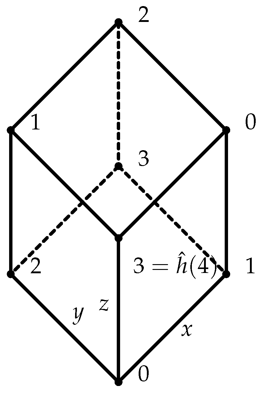
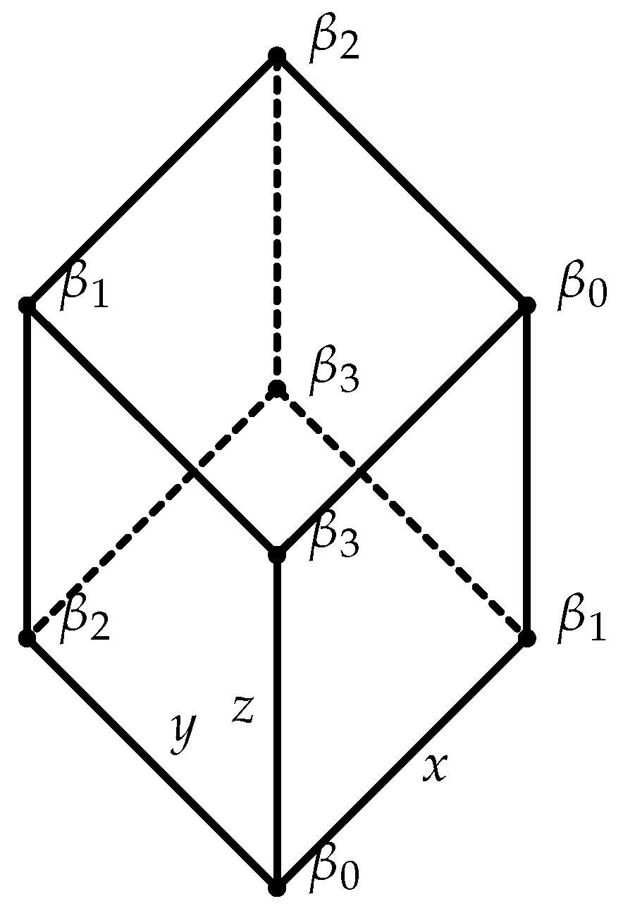
Example 2

([23]). Let $g:{\{{\alpha }_0,{\alpha }_1\}}^3\to \{{\beta }_0,{\beta }_1,{\beta }_2,{\beta }_3\}$ (Figure 1) be a function such that

$$\begin{array}{c}\hfill g:({\alpha }_0,{\alpha }_0,{\alpha }_0)\mapsto {\beta }_0;g:({\alpha }_0,{\alpha }_0,{\alpha }_1)\mapsto {\beta }_3;\\ \hfill g:({\alpha }_0,{\alpha }_1,{\alpha }_0)\mapsto {\beta }_2;g:({\alpha }_0,{\alpha }_1,{\alpha }_1)\mapsto {\beta }_1;\\ \hfill g:({\alpha }_1,{\alpha }_0,{\alpha }_0)\mapsto {\beta }_1;g:({\alpha }_1,{\alpha }_0,{\alpha }_1)\mapsto {\beta }_0;\\ \hfill g:({\alpha }_1,{\alpha }_1,{\alpha }_0)\mapsto {\beta }_3;g:({\alpha }_1,{\alpha }_1,{\alpha }_1)\mapsto {\beta }_2.\end{array}$$

(94)

Define $\mu :\{{\alpha }_0,{\alpha }_1\}\to {\mathbb{Z}}_4$ and $\nu :\{{\beta }_0,{\beta }_1,{\beta }_2,{\beta }_3\}\to {\mathbb{Z}}_4$ by

$$\begin{array}{cccc}\hfill \mu & :{\alpha }_j\mapsto j,\hfill & \hfill \forall & j\in \{0,1\},and\hfill \\ \hfill \nu & :{\beta }_j\mapsto j,\hfill & \hfill \forall & j\in \{0,1,2,3\},\hfill \end{array}$$

(95)

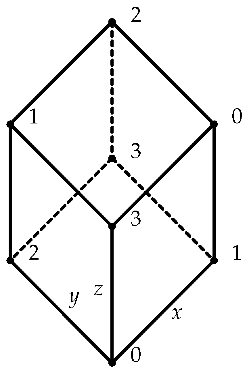
respectively. Obviously, g is equivalent to $x+2y+3z\in {\mathbb{Z}}_4\left[3\right]$ (Figure 2) via ${\mu }_1={\mu }_2={\mu }_3=\mu$ and ν. However, by Proposition 4, there exists no $\widehat{g}\in {\mathbb{F}}_4\left[3\right]$ of format (78) so that g is equivalent to any restriction of $\widehat{g}$. Although, Lemma 5 ensures that there always exists a bigger field ${\mathbb{F}}_q$ such that g admits a presentation $\widehat{g}\in {\mathbb{F}}_q\left[3\right]$ of format (78), the size q must be strictly bigger than 4. For instance, let

$$\begin{array}{c}\hfill \widehat{h}\left(x\right)=\sum _{a\in {\mathbb{Z}}_5}a\left[1-{(x-a)}^4\right]-\left[1-{(x-4)}^4\right]\in {\mathbb{Z}}_5\left[1\right].\end{array}$$

(96)

Then, g has presentation $\widehat{h}(x+2y+4z)\in {\mathbb{Z}}_5\left[3\right]$ (Figure 3) via ${\mu }_1={\mu }_2={\mu }_3=\mu :\{{\alpha }_0,{\alpha }_1\}\to {\mathbb{Z}}_5$ and $\nu :\{{\beta }_0,{\beta }_1,{\beta }_2,{\beta }_3\}\to {\mathbb{Z}}_5$ defined (symbolic-wise) by (95).

Proposition 4.

There exists no polynomial function $\widehat{g}\in {\mathbb{F}}_4\left[3\right]$ of format (78), such that a restriction of $\widehat{g}$ is equivalent to the function g defined by (94).

Proof. 

Suppose $\nu \circ g=\widehat{g}\circ ({\mu }_1,{\mu }_2,{\mu }_3)$, where ${\mu }_1,{\mu }_1,{\mu }_3:\{{\alpha }_0,{\alpha }_1\}\to {\mathbb{F}}_4$, $\nu :\{{\beta }_0,\cdots ,{\beta }_3\}\to {\mathbb{F}}_4$ are injections, and $\widehat{g}=h\circ (k_1+k_2+k_3)$ with $h,k_i\in {\mathbb{F}}_4\left[1\right]$ for all feasible i. We claim that $\widehat{g}$ and h are both surjective, since $\left|g\left({\{{\alpha }_0,{\alpha }_1\}}^3\right)\right|=\left|\{{\beta }_0,{\beta }_1,{\beta }_2,{\beta }_3\}\right|=4=\left|{\mathbb{F}}_4\right|.$ In particular, h is bijective. Therefore, $h^{-1}\circ \nu \circ g=k_1\circ {\mu }_1+k_2\circ {\mu }_2+k_3\circ {\mu }_3$, i.e., g admits a presentation $k_1\left(x\right)+k_2\left(y\right)+k_3\left(z\right)\in {\mathbb{F}}_4\left[3\right]$. A contradiction to Lemma A3. ☐

As a consequence of Proposition 4, in the sense of Körner–Marton, in order to use LCoF to encode function g, the alphabet sizes of the three encoders need to be at least 5. However, LCoR offers a solution in which the alphabet sizes are 4, strictly smaller than using LCoF. Most importantly, the region achieved with linear coding over any finite field ${\mathbb{F}}_q$, is always a subset of the one achieved with linear coding over ${\mathbb{Z}}_4$. This is proved in the following proposition.

Proposition 5.

Let g be the function defined by (94), ${\{{\alpha }_0,{\alpha }_1\}}^3$ be the sample space of $(X_1,X_2,X_3)\sim p$ and $p_X$ be the distribution of $X=g(X_1,X_2,X_3)$. If

$$\begin{array}{c}\hfill p_X\left({\beta }_0\right)=p_1,p_X\left({\beta }_1\right)=p_2,p_X\left({\beta }_3\right)=p_{3}and{p}_X\left({\beta }_2\right)=p_4\end{array}$$

(97)

satisfying (89), then, in the sense of Körner–Marton, the region ${\mathcal{R}}_1$ achieved with linear coding over ${\mathbb{Z}}_4$ contains the one, that is ${\mathcal{R}}_2$, obtained with linear coding over any finite field ${\mathbb{F}}_q$ for computing g. Moreover, if $\mathrm{supp}\left(p\right)$ is the whole domain of g, then ${\mathcal{R}}_1⊋{\mathcal{R}}_2$.

Proof. 

Let $\widehat{g}=h\circ k\in {\mathbb{F}}_q\left[3\right]$ be a polynomial presentation of g with format (78). By Corollary 2 and Remark 20, we have

$$\begin{array}{cc}\hfill {\mathcal{R}}_1=& \left\{\left.(R_1,R_2,R_3)\in {\mathbb{R}}^3\right|R_i>H(X_1+2X_2+3X_3)\right\},\hfill \end{array}$$

(98)

$$\begin{array}{cc}\hfill {\mathcal{R}}_2=& \left\{\left.(R_1,R_2,R_3)\in {\mathbb{R}}^3\right|R_i>H\left(k(X_1,X_2,X_3)\right)\right\}.\hfill \end{array}$$

(99)

Assume that $\nu \circ g=h\circ k\circ ({\mu }_1,{\mu }_2,{\mu }_3)$, where ${\mu }_1,{\mu }_1,{\mu }_3:\{{\alpha }_0,{\alpha }_1\}\to {\mathbb{F}}_q$ and $\nu :\{{\beta }_0,\cdots ,{\beta }_3\}\to {\mathbb{F}}_q$ are injections. Obviously, $g(X_1,X_2,X_3)$ is a function of $k(X_1,X_2,X_3)$. Hence,

$$\begin{array}{c}\hfill H\left(k(X_1,X_2,X_3)\right)\ge H\left(g(X_1,X_2,X_3)\right).\end{array}$$

(100)

On the other hand, $H(X_1+2X_2+3X_3)=H\left(g(X_1,X_2,X_3)\right)$. Therefore,

$$\begin{array}{c}\hfill H\left(k(X_1,X_2,X_3)\right)\ge H(X_1+2X_2+3X_3),\end{array}$$

(101)

and ${\mathcal{R}}_1\supseteq {\mathcal{R}}_2$. In addition, we claim that ${h|}_{\mathcal{S}}$, where $\mathcal{S}=k\left({\prod }_{j=1}^3{\mu }_j\{{\alpha }_0,{\alpha }_1\}\right)$, is not injective. Otherwise, $h:\mathcal{S}\to {\mathcal{S}}^{\prime }$, where ${\mathcal{S}}^{\prime }=h\left(\mathcal{S}\right)$, is bijective, hence, ${\left({h|}_{{\mathcal{S}}^{\prime }}\right)}^{-1}\circ \nu \circ g=k\circ ({\mu }_1,{\mu }_2,{\mu }_3)=k_1\circ {\mu }_1+k_2\circ {\mu }_2+k_3\circ {\mu }_3$. A contradiction to Lemma A3. Consequently, $\left|\mathcal{S}\right|>\left|{\mathcal{S}}^{\prime }\right|=\left|\nu \left(\{{\beta }_0,\cdots ,{\beta }_3\}\right)\right|=4$. If $\mathrm{supp}\left(p\right)={\{{\alpha }_0,{\alpha }_1\}}^3$, then (100) as well as (101) hold strictly, thus, ${\mathcal{R}}_1⊋{\mathcal{R}}_2$. ☐

A more intuitive comparison (which is not as conclusive as Proposition 5) can be identified from the presentations of g given in Figure 2 and Figure 3. According to Corollary 2, linear encoders over field ${\mathbb{Z}}_5$ achieve

$$\begin{array}{c}\hfill {\mathcal{R}}_{{\mathbb{Z}}_5}=\left\{\left.(R_1,R_2,R_3)\in {\mathbb{R}}^3\right|R_i>H(X_1+2X_2+4X_3)\right\}.\end{array}$$

(102)

The one achieved by linear encoders over ring ${\mathbb{Z}}_4$ is

$$\begin{array}{c}\hfill {\mathcal{R}}_{{\mathbb{Z}}_4}=\left\{\left.(R_1,R_2,R_3)\in {\mathbb{R}}^3\right|R_i>H(X_1+2X_2+3X_3)\right\}.\end{array}$$

(103)

Clearly, $H(X_1+2X_2+3X_3)\le H(X_1+2X_2+4X_3)$, thus, ${\mathcal{R}}_{{\mathbb{Z}}_4}$ contains ${\mathcal{R}}_{{\mathbb{Z}}_5}$. Furthermore, as long as

$$\begin{array}{c}\hfill 0<Pr\left({\alpha }_0,{\alpha }_0,{\alpha }_1\right),Pr\left({\alpha }_1,{\alpha }_1,{\alpha }_0\right)<1,\end{array}$$

(104)

${\mathcal{R}}_{{\mathbb{Z}}_4}$ is strictly larger than ${\mathcal{R}}_{{\mathbb{Z}}_5}$, since $H(X_1+2X_2+3X_3)<H(X_1+2X_2+4X_3)$. To be specific, assume that $(X_1,X_2,X_3)\sim p$ satisfies

Table 1. Distribution p.

$({\mathit{X}}_{\mathbf{1}},{\mathit{X}}_{\mathbf{2}},{\mathit{X}}_{\mathbf{3}})$	$\mathit{p}$	$({\mathit{X}}_{\mathbf{1}},{\mathit{X}}_{\mathbf{2}},{\mathit{X}}_{\mathbf{3}})$	$\mathit{p}$
$({\alpha }_0,{\alpha }_0,{\alpha }_0)$	$1/90$	$({\alpha }_0,{\alpha }_1,{\alpha }_0)$	$1/90$
$({\alpha }_1,{\alpha }_0,{\alpha }_1)$	$1/90$	$({\alpha }_1,{\alpha }_1,{\alpha }_1)$	$1/90$
$({\alpha }_1,{\alpha }_0,{\alpha }_0)$	$42/90$	$({\alpha }_0,{\alpha }_0,{\alpha }_1)$	$1/90$
$({\alpha }_0,{\alpha }_1,{\alpha }_1)$	$42/90$	$({\alpha }_1,{\alpha }_1,{\alpha }_0)$	$1/90$

, we have

$$\begin{array}{cc}\hfill \mathcal{R}[X_1,X_2,X_3]⊊& {\mathcal{R}}_{{\mathbb{Z}}_5}=\left\{\left.(R_1,R_2,R_3)\in {\mathbb{R}}^3\right|R_i>0.4812\right\}\hfill \end{array}$$

(105)

$$\begin{array}{cc}\hfill ⊊& {\mathcal{R}}_{{\mathbb{Z}}_4}=\left\{\left.(R_1,R_2,R_3)\in {\mathbb{R}}^3\right|R_i>0.4590\right\}.\hfill \end{array}$$

(106)

Based on Propositions 4 and 5, we conclude that LCoR dominates LCoF, in terms of achieving better coding rates with smaller alphabet sizes of the encoders for computing g. As a direct conclusion, we have:

Theorem 12.

In the sense of Körner–Marton, LCoF is not optimal.

Remark 23.

The key property underlying the proof of Proposition 5 is that the characteristic of a finite field must be a prime while the characteristic of a finite ring can be any positive integer larger than or equal to 2. This implies that it is possible to construct infinitely many discrete functions for which using LCoF always leads to a suboptimal achievable region compared to linear coding over finite non-field rings. Examples include ${\sum }_{i=1}^s{x}_i\in {\mathbb{Z}}_{2p}\left[s\right]$ for $s\ge 2$ and prime $p>2$ (note: the characteristic of ${\mathbb{Z}}_{2p}$ is $2p$ which is not a prime). One can always find an explicit distribution of sources for which linear coding over ${\mathbb{Z}}_{2p}$ strictly dominates linear coding over each and every finite field.

As mentioned, ${\mathcal{R}}_{\widehat{g}}$ given by (79) is sometimes strictly smaller than $\mathcal{R}\left[g\right]$. This was first shown by Ahlswede–Han [5] for the case of g being the modulo-two sum. Their approach combines the linear coding technique over a binary field with the standard random coding technique. In the following, we generalize the result of Ahlswede–Han ([5], Theorem 10) to the settings, where g is arbitrary, and, at the same time, LCoF is replaced by its generalized version, LCoR.

Consider function $\widehat{g}$ admitting

$$\begin{array}{c}\hfill \widehat{g}(x_1,x_2,\cdots ,x_s)=h\left[k_0(x_1,x_2,\cdots ,x_{s_0}),\sum _{j=s_0+1}^s{k}_j\left(x_j\right)\right],0\le s_0<s,\end{array}$$

(107)

where $k_0:{\mathfrak{R}}^{s_0}\to \mathfrak{R}$ and $h,k_j$’s are functions mapping $\mathfrak{R}$ to $\mathfrak{R}$. By Lemma 5, a discrete function with a finite domain is always equivalent to a restriction of some function of format (107). We call $\widehat{g}$ from (107) a pseudo nomographic function over ring $\mathfrak{R}$.

Theorem 13.

Let ${\mathcal{S}}_0=\{1,2,\cdots ,s_0\}\subseteq \mathcal{S}=\{1,2,\cdots ,s\}$. If $\widehat{g}$ is of format (107), and $\mathbf{R}=(R_1,R_2,\cdots ,R_s)\in {\mathbb{R}}^s$ satisfying

$$\begin{array}{c}\hfill \sum _{j\in T}{R}_j>\left|T\backslash {\mathcal{S}}_0\right|\underset{0\ne \mathfrak{I}{\le }_l\mathfrak{R}}{max}{\displaystyle \frac{log\left|\mathfrak{R}\right|}{log\left|\mathfrak{I}\right|}}\left[H\left(X\right|V_{\mathcal{S}})-H\left(Y_{\mathfrak{R}/\mathfrak{I}}\right|V_{\mathcal{S}})\right]+I(Y_T;V_T|V_{T^c}),\forall \varnothing \ne T\subseteq \mathcal{S},\end{array}$$

(108)

where $\forall j\in {\mathcal{S}}_0$, $V_j=Y_j=X_j$; $\forall j\in \mathcal{S}\backslash {\mathcal{S}}_0$, $Y_j=k_j\left(X_j\right)$, $V_j$’s are discrete random variables such that

$$\begin{array}{c}\hfill p(y_1,y_2,\cdots ,y_s,v_1,v_2,\cdots ,v_s)=p(y_1,y_2,\cdots ,y_s)\prod _{j=s_0+1}^{s}p\left(v_j\right|y_j),\end{array}$$

(119)

and $X={\sum }_{j=s_0+1}^s{Y}_j$, $Y_{\mathfrak{R}/\mathfrak{I}}=X+\mathfrak{I}$, then $\mathbf{R}\in \mathcal{R}\left[\widehat{g}\right]$.

Proof. 

The proof can be completed by applying the tricks from Lemmas 2 and 3 to the approach generalized from Ahlswede–Han ([5], Theorem 10). Details are found in Appendix C. ☐

Remark 24.

The achievable region given by (108) always contains the SW region. Moreover, it is in general larger than the ${\mathcal{R}}_{\widehat{g}}$ from (79). If $\widehat{g}$ is the modulo-two sum, namely $s_0=0$ and $h,k_j$’s are identity functions for all $s_0<j\le s$, then (108) resumes the region of Ahlswede–Han ([5], Theorem 10).

7. Conclusions

7.1. Right Linearity

Careful readers might have noticed that the encoders we used so far are actually left linear mappings. By symmetry, almost all related statements can be easily reproved for right linear mappings (encoders). As an example, the following corresponds to Theorem 2.

Theorem 14.

For any $\mathsf{\Phi }\in \mathcal{M}\left({\mathcal{X}}_{\mathcal{S}},{\mathfrak{R}}_{\mathcal{S}}\right)$,

$$\begin{array}{c}\hfill {\mathcal{R}}_{\mathsf{\Phi }}^{\prime }=\left\{\left(R_1,R_2,\cdots ,R_s\right)\in {\mathbb{R}}^s|\sum _{i\in T}{\displaystyle \frac{R_{i}log\left|{\mathfrak{I}}_i\right|}{log|{\mathfrak{R}}_i|}}>r\left(T,{\mathfrak{I}}_T\right),\forall \varnothing \ne T\subseteq \mathcal{S},\forall 0\ne {\mathfrak{I}}_i{\le }_r{\mathfrak{R}}_i\right\},\end{array}$$

(110)

where $r\left(T,{\mathfrak{I}}_T\right)=H\left(X_T\right|X_{T^c})-H\left(Y_{{\mathfrak{R}}_T/{\mathfrak{I}}_T}\right|X_{T^c})$ and $Y_{{\mathfrak{R}}_T/{\mathfrak{I}}_T}=\mathsf{\Phi }\left(X_T\right)+{\mathfrak{I}}_T$, is achievable with (right) linear coding over the finite rings ${\mathfrak{R}}_1,{\mathfrak{R}}_2,\cdots ,{\mathfrak{R}}_s$.

By time sharing,

$$\begin{array}{c}\hfill {\mathcal{R}}_r=\mathrm{cov}\left(\bigcup _{\mathsf{\Phi }\in \mathcal{M}\left({\mathcal{X}}_{\mathcal{S}},{\mathfrak{R}}_{\mathcal{S}}\right)}{\mathcal{R}}_{\mathsf{\Phi }}^{\prime }\right),\end{array}$$

(111)

where ${\mathcal{R}}_{\mathsf{\Phi }}^{\prime }$ is given by (110), is achievable with (right) LCoR.

7.2. Field, Ring, Rng and Group

Conceptually speaking, LCoR is in fact a generalization of the linear coding technique proposed by Elias [2] and Csiszár [3] (LCoF), since a field must be a ring. However, as seen in Section 4, analyzing the decoding error for the ring version is in general substantially more challenging than in the case of the field version. Our approach crucially relies on the concept of ideals. A field contains no non-trivial ideal but itself. Because of this special property of fields, our general argument for finite rings will render to a simple one when only finite fields are considered.

Even though our analysis for the ring scenario is more complicated than that for finite field scenarios, linear encoders working over some finite rings are in general considerably easier to implement in practice. This is because the implementation of finite field arithmetic can be quite demanding. Normally, a finite field is given by its polynomial representation, operations are carried out based on the polynomial operations (addition and multiplication) followed by the polynomial long division algorithm. In contrast, implementing arithmetic of many finite rings is a straightforward task. For instance, the arithmetic of modulo integers ring ${\mathbb{Z}}_q$, for any positive integer q, is simply the integer modulo q arithmetic.

In addition, it is also very interesting to consider instead linear coding over rngs. It will be even more intriguing should it turn out that the rng version outperforms the ring version in the computing problem (Problem 1), in the same manner that the ring version outperforms its field counterpart. It will also be interesting to see whether the idea of using rng provides more understanding of the problems from [6,8].

Some works, including [24,25,26], have proposed to implement coding over a simpler algebraic structure, that of a group. Seemingly, this corresponds to a more universal approach since both fields and rings are also groups. However, one subtle issue is often overlooked in this context. Namely, the set of rings (or rngs) is not a subset of the set of groups, since several non-isomorphic rings (or rngs) can be defined on one and the same group. For instance, given two distinct primes p and q, up to isomorphism,

• there are 2 finite rngs of order p, while there is only one group of order p;
• there are 4 finite rngs of order $pq$;
• there are 11 finite rngs of order $p^2$ (if $p=2$, then 4 of them are rings, namely ${\mathbb{F}}_4$, ${\mathbb{Z}}_4$, ${\mathbb{Z}}_2\times {\mathbb{Z}}_2$ and ${\mathbb{M}}_{L,2}$ [27]), while there are only 2 groups of order $p^2$, both of which are Abelian;
• there are 22 finite rngs of order $p^{2}q$;
• there are 52 finite rngs of order 8;
• there are $3p+50$ finite rngs of order $p^3$ ($p>2$), while there are 5 groups of order $p^3$, 3 of which are Abelian.

Therefore, there is no one-to-one correspondence between rings (field or rngs) and groups, in either direction. Furthermore, from the point of view of formulating a multivariate function, one is highly restricted by using groups, compared to rings (rng or field). Specifically, it is well-known that every discrete function defined on a finite domain is essentially a restriction of some polynomial function over a finite ring (rng or field). Although non-Abelian structures (non-Abelian groups) have the potential to lead to important non-trivial results [28], they are very difficult to handle theoretically and in practice. The performance of non-Abelian group block codes can be quite bad [29].

7.3. Final Remarks

This paper establishes achievability theorems regarding linear coding over finite rings for Slepian–Wolf data compression. Our results include related work from Elias [2] and Csiszár [3] regarding linear coding over finite fields as special cases in the sense of characterizing the achievable region. We have also proved that, for any Slepian–Wolf scenario, there always exists a sequence of linear encoders over some finite rings (non-field rings in particular) that achieves the data compression limit, the Slepian–Wolf region. Thus, with regard to existence, the optimality issue of linear coding over finite non-field rings for data compression is confirmed positively.

In addition, we also address the problem of source coding for computing, Problem 1. Results of Körner–Marton [4], Ahlswede–Han ([5], Theorem 10) and [7] are generalized to corresponding ring versions. Based on these, it is demonstrated that LCoR dominates its field counterpart for encoding (infinitely) many discrete functions.

References

- Slepian, D.; Wolf, J.K. Noiseless Coding of Correlated Information Sources. IEEE Trans. Inf. Theory 1973, 19, 471–480. [Google Scholar] [CrossRef]
- Elias, P. Coding for Noisy Channels. IRE Conv. Rec. 1955, 3, 37–46. [Google Scholar]
- Csiszár, I. Linear Codes for Sources and Source Networks: Error Exponents, Universal Coding. IEEE Trans. Inf. Theory 1982, 28, 585–592. [Google Scholar] [CrossRef]
- Körner, J.; Marton, K. How to Encode The Modulo-Two Sum of Binary Sources. IEEE Trans. Inf. Theory 1979, 25, 219–221. [Google Scholar] [CrossRef]
- Ahlswede, R.; Han, T.S. On Source Coding with Side Information via a Multiple-Access Channel and Related Problems in Multi-User Information Theory. IEEE Trans. Inf. Theory 1983, 29, 396–411. [Google Scholar] [CrossRef]
- Huang, S.; Skoglund, M. Polynomials and Computing Functions of Correlated Sources. In Proceedings of the 2012 IEEE International Symposium on Information Theory, Cambridge, MA, USA, 1–6 July 2012; pp. 771–775. [Google Scholar]
- Huang, S.; Skoglund, M. Computing Polynomial Functions of Correlated Sources: Inner Bounds. In Proceedings of the International Symposium on Information Theory and Its Applications, Honolulu, HI, USA, 28–31 October 2012; pp. 160–164. [Google Scholar]
- Han, T.S.; Kobayashi, K. A Dichotomy of Functions F(X, Y) of Correlated Sources (X, Y) from the Viewpoint of the Achievable Rate Region. IEEE Trans. Inf. Theory 1987, 33, 69–76. [Google Scholar] [CrossRef]
- Como, G.; Fagnani, F. The Capacity of Finite Abelian Group Codes over Symmetric Memoryless Channels. IEEE Trans. Inf. Theory 2009, 55, 2037–2054. [Google Scholar] [CrossRef]
- Como, G. Group codes outperform binary-coset codes on nonbinary symmetric memoryless channels. IEEE Trans. Inf. Theory 2010, 56, 4321–4334. [Google Scholar] [CrossRef]
- Krithivasan, D.; Pradhan, S. Distributed Source Coding Using Abelian Group Codes: A New Achievable Rate-Distortion Region. IEEE Trans. Inf. Theory 2011, 57, 1495–1519. [Google Scholar] [CrossRef]
- Rotman, J.J. Advanced Modern Algebra, 2nd ed.; American Mathematical Society: Providence, RI, USA, 2010. [Google Scholar]
- Mullen, G.; Stevens, H. Polynomial functions (modm). Acta Math. Hung. 1984, 44, 237–241. [Google Scholar] [CrossRef]
- Hungerford, T.W. Algebra (Graduate Texts in Mathematics); Springer: New York, NY, USA, 1980. [Google Scholar]
- Lam, T.Y. A First Course in Noncommutative Rings, 2nd ed.; Springer: New York, NY, USA, 2001. [Google Scholar]
- Dummit, D.S.; Foote, R.M. Abstract Algebra, 3rd ed.; Wiley: New York, NY, USA, 2003. [Google Scholar]
- Anderson, F.W.; Fuller, K.R. Rings and Categories of Modules, 2nd ed.; Springer: New York, NY, USA, 1992. [Google Scholar]
- Yeung, R.W. Information Theory and Network Coding, 1st ed.; Springer: New York, NY, USA, 2008. [Google Scholar]
- Cover, T.M.; Thomas, J.A. Elements of Information Theory, 2nd ed.; Wiley: New York, NY, USA, 2006. [Google Scholar]
- Huang, S.; Skoglund, M. On achievability of linear source coding over finite rings. In Proceedings of the 2013 IEEE International Symposium on Information Theory Proceedings (ISIT), Istanbul, Turkey, 7–12 July 2013; pp. 1984–1988. [Google Scholar]
- Huang, S.; Skoglund, M. Encoding Irreducible Markovian Functions of Sources: An Application of Supremus Typicality; KTH Royal Institute of Technology: Stockholm, Sweden, 2013. [Google Scholar]
- Buck, R.C. Nomographic Functions are Nowhere Dense. Proc. Am. Math. Soc. 1982, 85, 195–199. [Google Scholar] [CrossRef]
- Huang, S.; Skoglund, M. Linear Source Coding over Rings and Applications. In Proceedings of the IEEE Swedish Communication Technologies Workshop, Lund, Sweden, 24–26 October 2012; pp. 1–6. [Google Scholar]
- Slepian, D. Group Codes for the Gaussian Channel. Bell Syst. Tech. J. 1968, 47, 575–602. [Google Scholar] [CrossRef]
- Ahlswede, R. Group Codes do not Achieve Shannon’s Channel Capacity for General Discrete Channels. Ann. Math. Stat. 1971, 42, 224–240. [Google Scholar] [CrossRef]
- Forney, G.D., Jr. On the Hamming distance properties of group codes. IEEE Trans. Inf. Theory 1992, 38, 1797–1801. [Google Scholar] [CrossRef]
- Singmaster, D.; Bloom, D.M. Rings of Order Four. Math. Assoc. Am. 1964, 71, 918–920. [Google Scholar] [CrossRef]
- Chan, T.H.; Grant, A. Entropy vector and network codes. In Proceedings of the IEEE International Symposium on Information Theory, Nice, France, 24–29 June 2007. [Google Scholar]
- Interlando, J.C.; Palazzo, R., Jr.; Elia, M. Group Block Codes Over Nonabelian Groups are Asymptotically Bad. IEEE Trans. Inf. Theory 1996, 42, 1277–1280. [Google Scholar] [CrossRef]
- Du, J.; KTH Royal Institute of Technology, Stockholm, Sweden; Andersson, M.; KTH Royal Institute of Technology, Stockholm, Sweden. Personal Communication, 2012.
- Lidl, R.; Niederreiter, H. Finite Fields, 2nd ed.; Gambridge University Press: New York, NY, USA, 1997. [Google Scholar]