
New Insights into the State Trapping of UV-Excited Thymine

Abstract
:
1. Introduction
2. Results
2.1. Topography of Excited States
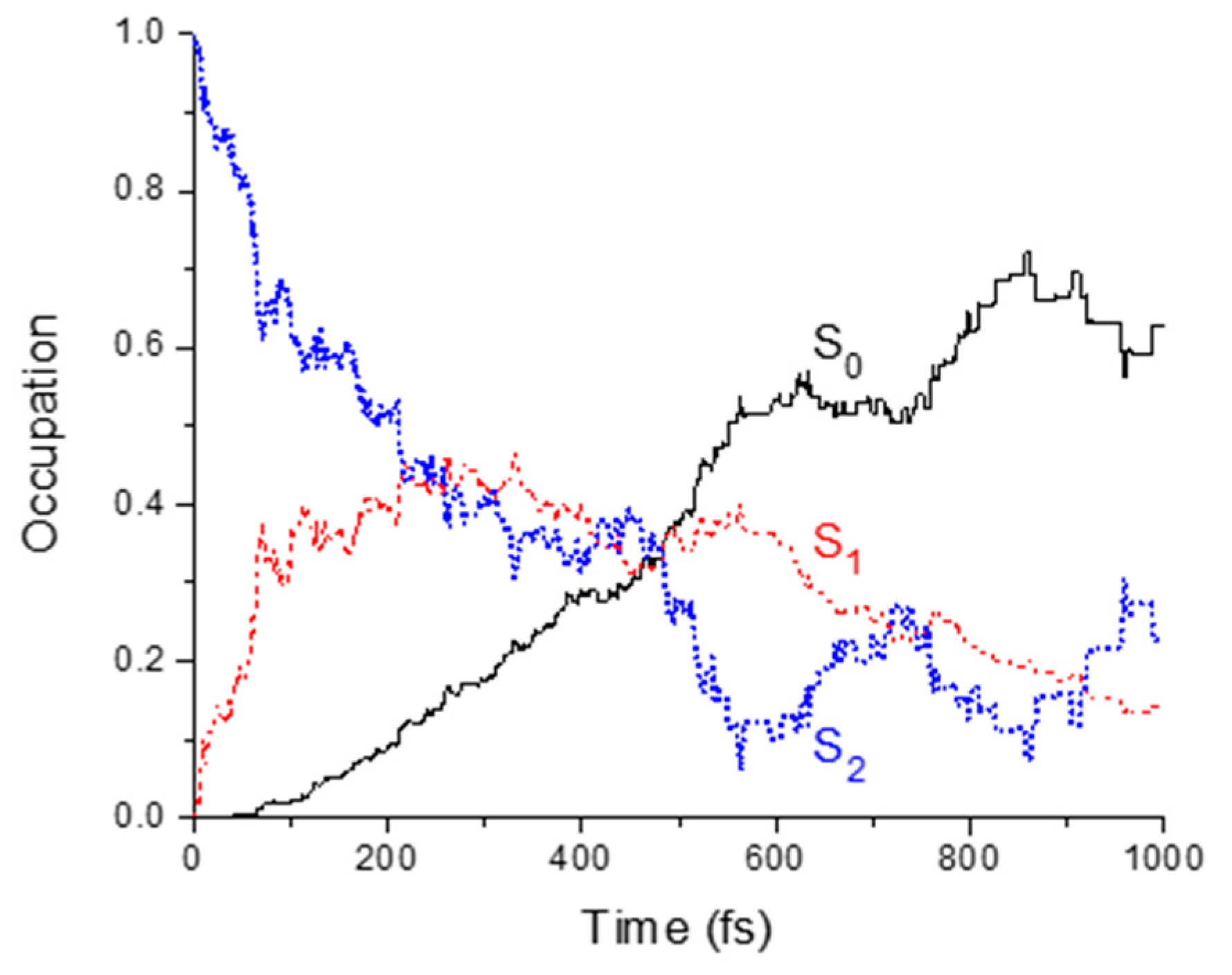
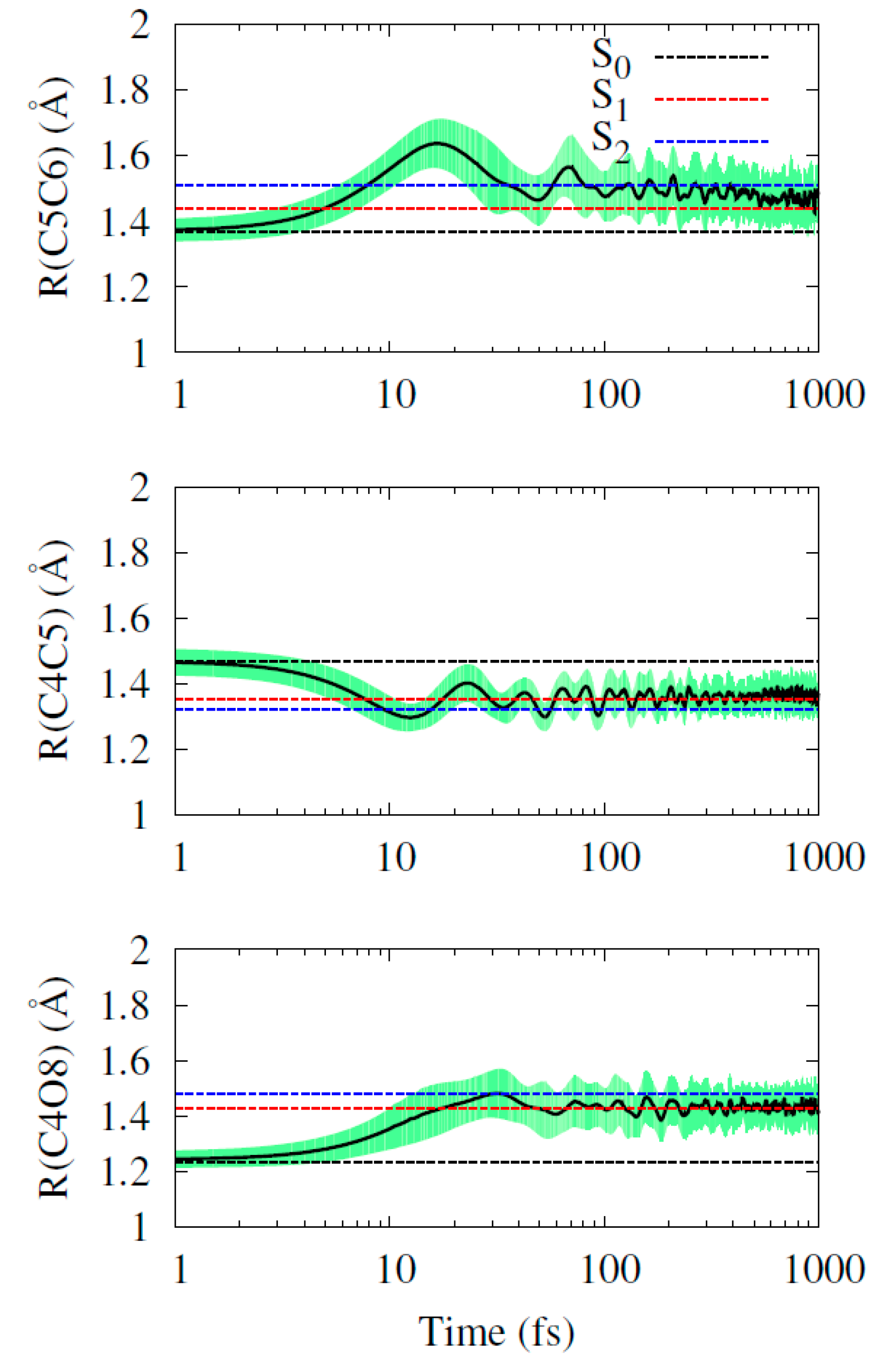
2.2. Dynamics
3. Discussion
4. Theoretical and Computational Details
4.1. Potential Energy, Spectrum, and Dynamics Simulations
4.2. OD Method for Coupling Calculations
Supplementary Materials
Acknowledgments
Author Contributions
Conflicts of Interest
References
- Yu, H.; Sanchez-Rodriguez, J.A.; Pollum, M.; Crespo-Hernandez, C.E.; Mai, S.; Marquetand, P.; Gonzalez, L.; Ullrich, S. Internal conversion and intersystem crossing pathways in uv excited, isolated uracils and their implications in prebiotic chemistry. Phys. Chem. Chem. Phys. 2016, 18, 20168–20176. [Google Scholar] [CrossRef] [PubMed]
- Kang, H.; Lee, K.T.; Jung, B.; Ko, Y.J.; Kim, S.K. Intrinsic lifetimes of the excited state of DNA and RNA bases. J. Am. Chem. Soc. 2002, 124, 12958–12959. [Google Scholar] [CrossRef] [PubMed]
- Ullrich, S.; Schultz, T.; Zgierski, M.Z.; Stolow, A. Electronic relaxation dynamics in DNA and RNA bases studied by time-resolved photoelectron spectroscopy. Phys. Chem. Chem. Phys. 2004, 6, 2796–2801. [Google Scholar] [CrossRef]
- McFarland, B.K.; Farrell, J.P.; Miyabe, S.; Tarantelli, F.; Aguilar, A.; Berrah, N.; Bostedt, C.; Bozek, J.D.; Bucksbaum, P.H.; Castagna, J.C.; et al. Ultrafast X-ray auger probing of photoexcited molecular dynamics. Nat. Commun. 2014, 5, 4235. [Google Scholar] [CrossRef] [PubMed]
- Gonzalez-Vazquez, J.; Gonzalez, L.; Samoylova, E.; Schultz, T. Thymine relaxation after uv irradiation: The role of tautomerization and πσ* states. Phys. Chem. Chem. Phys. 2009, 11, 3927–3934. [Google Scholar] [CrossRef] [PubMed]
- Gador, N.; Samoylova, E.; Smith, V.R.; Stolow, A.; Rayner, D.M.; Radloff, W.; Hertel, I.V.; Schultz, T. Electronic structure of adenine and thymine base pairs studied by femtosecond electron-ion coincidence spectroscopy. J. Phys. Chem. A 2007, 111, 11743–11749. [Google Scholar] [CrossRef] [PubMed]
- Canuel, C.; Mons, M.; Piuzzi, F.; Tardivel, B.; Dimicoli, I.; Elhanine, M. Excited states dynamics of DNA and RNA bases: Characterization of a stepwise deactivation pathway in the gas phase. J. Chem. Phys. 2005, 122, 074316. [Google Scholar] [CrossRef] [PubMed]
- Samoylova, E.; Schultz, T.; Hertel, I.V.; Radloff, W. Analysis of ultrafast relaxation in photoexcited DNA base pairs of adenine and thymine. Chem. Phys. 2008, 347, 376–382. [Google Scholar] [CrossRef]
- Ligare, M.; Siouri, F.; Bludsky, O.; Nachtigallova, D.; de Vries, M.S. Characterizing the dark state in thymine and uracil by double resonant spectroscopy and quantum computation. Phys. Chem. Chem. Phys. 2015, 17, 24336–24341. [Google Scholar] [CrossRef] [PubMed]
- Samoylova, E.; Lippert, H.; Ullrich, S.; Hertel, I.V.; Radloff, W.; Schultz, T. Dynamics of photoinduced processes in adenine and thymine base pairs. J. Am. Chem. Soc. 2005, 127, 1782–1786. [Google Scholar] [CrossRef] [PubMed]
- Barbatti, M.; Borin, A.; Ullrich, S. Photoinduced processes in nucleic acids. In Photoinduced Phenomena in Nucleic Acids I; Barbatti, M., Borin, A.C., Ullrich, S., Eds.; Springer International Publishing: Cham, Switzerland, 2015; Volume 355, pp. 1–32. [Google Scholar]
- Yamazaki, S.; Taketsugu, T. Nonradiative deactivation mechanisms of uracil, thymine, and 5-fluorouracil: A comparative ab initio study. J. Phys. Chem. A 2012, 116, 491–503. [Google Scholar] [CrossRef] [PubMed]
- Perun, S.; Sobolewski, A.L.; Domcke, W. Conical intersections in thymine. J. Phys. Chem. A 2006, 110, 13238–13244. [Google Scholar] [CrossRef] [PubMed]
- Szymczak, J.J.; Barbatti, M.; Soo Hoo, J.T.; Adkins, J.A.; Windus, T.L.; Nachtigallová, D.; Lischka, H. Photodynamics simulations of thymine: Relaxation into the first excited singlet state. J. Phys. Chem. A 2009, 113, 12686–12693. [Google Scholar] [CrossRef] [PubMed]
- Zechmann, G.; Barbatti, M. Photophysics and deactivation pathways of thymine. J. Phys. Chem. A 2008, 112, 8273–8279. [Google Scholar] [CrossRef] [PubMed]
- Serrano-Pérez, J.J.; González-Luque, R.; Merchán, M.; Serrano-Andrés, L. On the intrinsic population of the lowest triplet state of thymine. J. Phys. Chem. B 2007, 111, 11880–11883. [Google Scholar] [CrossRef] [PubMed]
- Bai, S.; Barbatti, M. Why replacing different oxygens of thymine with sulfur causes distinct absorption and intersystem crossing. J. Phys. Chem. A 2016. [Google Scholar] [CrossRef] [PubMed]
- Merchán, M.; González-Luque, R.; Climent, T.; Serrano-Andrés, L.; Rodriuguez, E.; Reguero, M.; Pelaez, D. Unified model for the ultrafast decay of pyrimidine nucleobases. J. Phys. Chem. B 2006, 110, 26471–26476. [Google Scholar] [CrossRef] [PubMed]
- Asturiol, D.; Lasorne, B.; Robb, M.A.; Blancafort, L. Photophysics of the π,π* and n,π* states of thymine: Ms-CASPT2 minimum-energy paths and CASSCF on-the-fly dynamics. J. Phys. Chem. A 2009, 113, 10211–10218. [Google Scholar] [CrossRef] [PubMed]
- Lan, Z.; Fabiano, E.; Thiel, W. Photoinduced nonadiabatic dynamics of pyrimidine nucleobases: On-the-fly surface-hopping study with semiempirical methods. J. Phys. Chem. B 2009, 113, 3548–3555. [Google Scholar] [CrossRef] [PubMed]
- González, L.; González-Vázquez, J.; Samoylova, E.; Schultz, T. On the puzzling deactivation mechanism of thymine after light irradiation. AIP Conf. Proc. 2008, 1080, 169–175. [Google Scholar]
- Arbelo-González, W.; Crespo-Otero, R.; Barbatti, M. Steady and time-resolved photoelectron spectra based on nuclear ensembles. J. Chem. Theory Comput. 2016, 12, 5037–5049. [Google Scholar] [CrossRef] [PubMed]
- Hudock, H.R.; Levine, B.G.; Thompson, A.L.; Satzger, H.; Townsend, D.; Gador, N.; Ullrich, S.; Stolow, A.; Martínez, T.J. Ab initio molecular dynamics and time-resolved photoelectron spectroscopy of electronically excited uracil and thymine. J. Phys. Chem. A 2007, 111, 8500–8508. [Google Scholar] [CrossRef] [PubMed]
- Barbatti, M.; Aquino, A.J.A.; Szymczak, J.J.; Nachtigallová, D.; Hobza, P.; Lischka, H. Relaxation mechanisms of UV-photoexcited DNA and RNA nucleobases. Proc. Natl. Acad. Sci. USA 2010, 107, 21453–21458. [Google Scholar] [CrossRef] [PubMed]
- Picconi, D.; Barone, V.; Lami, A.; Santoro, F.; Improta, R. The interplay between ππ*/nπ* excited states in gas-phase thymine: A quantum dynamical study. ChemPhysChem 2011, 12, 1957–1968. [Google Scholar] [CrossRef] [PubMed]
- Cremer, D.; Pople, J.A. General definition of ring puckering coordinates. J. Am. Chem. Soc. 1975, 97, 1354–1358. [Google Scholar] [CrossRef]
- Zhu, X.-M.; Wang, H.-G.; Zheng, X.; Phillips, D.L. Role of ribose in the initial excited state structural dynamics of thymidine in water solution: A resonance raman and density functional theory investigation. J. Phys. Chem. B 2008, 112, 15828–15836. [Google Scholar] [CrossRef] [PubMed]
- Abouaf, R.; Pommier, J.; Dunet, H. Electronic and vibrational excitation in gas phase thymine and 5-bromouracil by electron impact. Chem. Phys. Lett. 2003, 381, 486–494. [Google Scholar] [CrossRef]
- Tuna, D.; Lefrancois, D.; Wolański, Ł.; Gozem, S.; Schapiro, I.; Andruniów, T.; Dreuw, A.; Olivucci, M. Assessment of approximate coupled-cluster and algebraic-diagrammatic-construction methods for ground- and excited-state reaction paths and the conical-intersection seam of a retinal-chromophore model. J. Chem. Theory Comput. 2015, 11, 5758–5781. [Google Scholar] [CrossRef] [PubMed]
- Trofimov, A.B.; Schirmer, J. An efficient polarization propagator approach to valence electron excitation spectra. J. Phys. B At. Mol. Opt. Phys. 1995, 28, 2299–2324. [Google Scholar] [CrossRef]
- Schirmer, J. Beyond the random-phase approximation: A new approximation scheme for the polarization propagator. Phys. Rev. A 1982, 26, 2395–2416. [Google Scholar] [CrossRef]
- Dunning, T.H., Jr. Gaussian basis sets for use in correlated molecular calculations. I. The atoms boron through neon and hydrogen. J. Chem. Phys. 1989, 90, 1007–1023. [Google Scholar] [CrossRef]
- Fogarasi, G.; Zhou, X.F.; Taylor, P.W.; Pulay, P. The calculation of abinitio molecular geometries—Efficient optimization by natural internal coordinates and empirical correction by offset forces. J. Am. Chem. Soc. 1992, 114, 8191–8201. [Google Scholar] [CrossRef]
- Crespo-Otero, R.; Barbatti, M. Spectrum simulation and decomposition with nuclear ensemble: Formal derivation and application to benzene, furan and 2-phenylfuran. Theor. Chem. Acc. 2012, 131, 1237. [Google Scholar] [CrossRef]
- Tully, J.C. Molecular-dynamics with electronic-transitions. J. Chem. Phys. 1990, 93, 1061–1071. [Google Scholar] [CrossRef]
- Granucci, G.; Persico, M. Critical appraisal of the fewest switches algorithm for surface hopping. J. Chem. Phys. 2007, 126, 134114. [Google Scholar] [CrossRef] [PubMed]
- Swope, W.C.; Andersen, H.C.; Berens, P.H.; Wilson, K.R. A computer-simulation method for the calculation of equilibrium-constants for the formation of physical clusters of molecules—Application to small water clusters. J. Chem. Phys. 1982, 76, 637–649. [Google Scholar] [CrossRef]
- Butcher, J. A modified multistep method for the numerical integration of ordinary differential equations. J. Assoc. Comput. Mach. 1965, 12, 124–135. [Google Scholar] [CrossRef]
- Boeyens, J.C.A. The conformation of six-membered rings. J. Chem. Crystallogr. 1978, 8, 317–320. [Google Scholar] [CrossRef]
- Ahlrichs, R.; Bär, M.; Häser, M.; Horn, H.; Kölmel, C. Electronic-structure calculations on workstation computers—The program system turbomole. Chem. Phys. Lett. 1989, 162, 165–169. [Google Scholar] [CrossRef]
- Barbatti, M.; Ruckenbauer, M.; Plasser, F.; Pittner, J.; Granucci, G.; Persico, M.; Lischka, H. Newton-X: A surface-hopping program for nonadiabatic molecular dynamics. WIREs Comput. Mol. Sci. 2014, 4, 26–33. [Google Scholar] [CrossRef]
- Barbatti, M.; Granucci, G.; Ruckenbauer, M.; Plasser, F.; Crespo-Otero, R.; Pittner, J.; Persico, M.; Lischka, H. Newton-X: A Package for Newtonian Dynamics Close to the Crossing Seam. 2013. Available online: http://www.Newtonx.Org (accessed on 1 September 2016).
- Levine, B.G.; Coe, J.D.; Martínez, T.J. Optimizing conical intersections without derivative coupling vectors: Application to multistate multireference second-order perturbation theory (MS-CASPT2). J. Phys. Chem. B 2008, 112, 405–413. [Google Scholar] [CrossRef] [PubMed]
- Spek, A.L. Single-crystal structure validation with the program platon. J. Appl. Crystallogr. 2003, 36, 7–13. [Google Scholar] [CrossRef]
- Hammes-Schiffer, S.; Tully, J.C. Proton-transfer in solution—Molecular-dynamics with quantum transitions. J. Chem. Phys. 1994, 101, 4657–4667. [Google Scholar] [CrossRef]
- Pittner, J.; Lischka, H.; Barbatti, M. Optimization of mixed quantum-classical dynamics: Time-derivative coupling terms and selected couplings. Chem. Phys. 2009, 356, 147–152. [Google Scholar] [CrossRef]
- Werner, U.; Mitrić, R.; Suzuki, T.; Bonačić-Koutecký, V. Nonadiabatic dynamics within the time dependent density functional theory: Ultrafast photodynamics in pyrazine. Chem. Phys. 2008, 349, 319–324. [Google Scholar] [CrossRef]
- Tapavicza, E.; Tavernelli, I.; Rothlisberger, U. Trajectory surface hopping within linear response time-dependent density-functional theory. Phys. Rev. Lett. 2007, 98, 023001–023004. [Google Scholar] [CrossRef] [PubMed]
- Ryabinkin, I.G.; Nagesh, J.; Izmaylov, A.F. Fast numerical evaluation of time-derivative nonadiabatic couplings for mixed quantum-classical methods. J. Phys. Chem. Lett. 2015, 6, 4200–4203. [Google Scholar] [CrossRef] [PubMed]
- Frisch, M.J.; Trucks, G.W.; Schlegel, H.B.; Scuseria, G.E.; Robb, M.A.; Cheeseman, J.R.; Scalmani, G.; Barone, V.; Mennucci, B.; Petersson, G.A.; et al. Gaussian 09, Revision D.01; Gaussian, Inc.: Wallingford, CT, USA, 2013. [Google Scholar]
- Casida, M. Time-dependent density functional response theory for molecules. In Recent Advances in Density Functional Methods, Part I; Chong, D., Ed.; World Scientific: Singapore, 1995; pp. 155–192. [Google Scholar]
- Barbatti, M.; Crespo-Otero, R. Surface hopping dynamics with dft excited states. In Density-Functional Methods for Excited States; Ferré, N., Filatov, M., Huix-Rotllant, M., Eds.; Springer International Publishing: Cham, Switzerland, 2016; pp. 415–444. [Google Scholar]
- Plasser, F.; Crespo-Otero, R.; Pederzoli, M.; Pittner, J.; Lischka, H.; Barbatti, M. Surface hopping dynamics with correlated single-reference methods: 9H-adenine as a case study. J. Chem. Theory Comput. 2014, 10, 1395–1405. [Google Scholar] [CrossRef] [PubMed]


| Pump (nm) | Probe (nm) | τ1 (fs) | τ2 (ps) | τ3 (ps) | τ4 (ns) | References |
|---|---|---|---|---|---|---|
| 250 | 200 | <50 | 0.49 | 6.4 | [3] | |
| 260 | 295 | 175 | 6.13 | >1 | [1] | |
| 266 | 2.19 (X-ray) | 200–300 | [4] | |||
| 266 | 400/800 | <100 | 7 | long | [5] | |
| 266 | 800 | 200 | 7 | [6] | ||
| 267 | 2 × 400 | 105 | 5.12 | [7] | ||
| 267 | 800 | 100 | 7 | >1 | [8] | |
| 267 | 800 | 6.4 | >100 | [2] | ||
| 270 | 193 | 293 | [9] | |||
| 272 | 800 | 130 | 6.5 | [10] |
| Geometry | State | Energy (eV) | ||
|---|---|---|---|---|
| ADC(2) | CASSCF a | MS-CASPT2 b | ||
| S0 min | S0 (cs) | 0.00 | 0.00 | 0.00 |
| S1 (nO4π*) | 4.56 | 5.19 | 5.09 | |
| S2 (πN1π*) | 5.06 | 6.87 | 5.09 | |
| S1 min | S0 (cs) | 1.33 | 1.39 | 1.02 |
| S1 (nO4π*) | 3.33 | 4.02 | 4.37 | |
| S2 min | S0 (cs) | 2.14 | 1.71 | 1.28 |
| S1 (nO4π*) | 3.50 | 4.18 | 4.51 | |
| S2 (πO4π*) | 4.18 | 5.64 | 4.77 | |
| X10 (nπ*/S0) | S0 (cs) | 3.90 | 5.02 | 5.02 |
| S1 (nO4π*) | 3.90 | 5.13 | 5.60 | |
| X10 (ππ*/S0) | S0 (cs) | 3.82 | 4.49 | 4.19 |
| S1 (π56π*) | 3.82 | 5.54 | 4.41 | |
| X21 (3,6B) | S0 (cs) | 3.37 | 2.68 | 2.23 |
| S1 (nO4π*) | 4.21 | 5.61 | 4.79 | |
| S2 (π56π*) | 4.22 | 6.00 | 5.63 | |
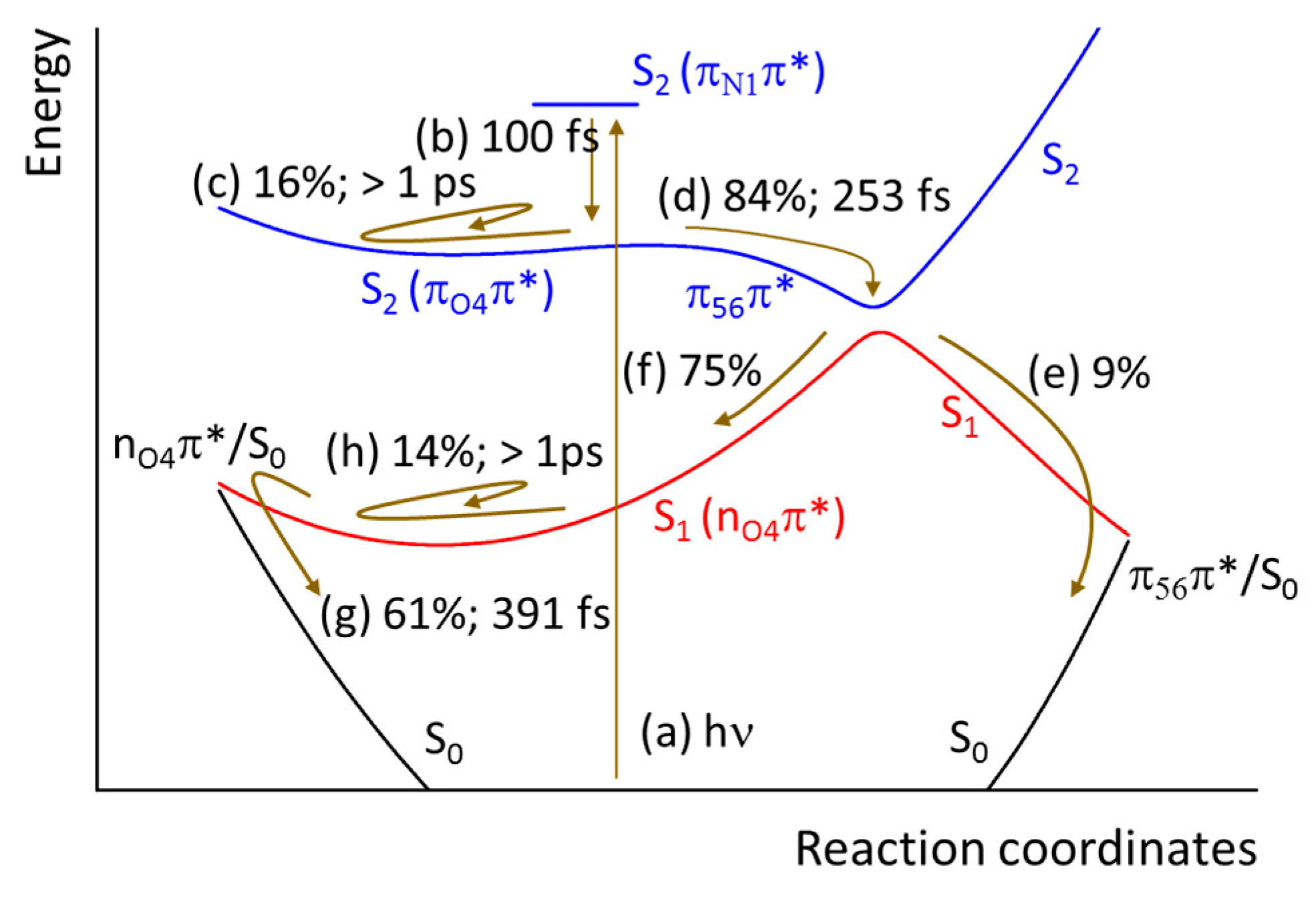
| Process | fτ | τ (fs) |
|---|---|---|
| FC → S2 min | 1.00 | ~100 |
| S2 → S1 | 0.84 | 253 |
| S1 → S0 | 0.70 | 391 |
© 2016 by the authors. Licensee MDPI, Basel, Switzerland. This article is an open access article distributed under the terms and conditions of the Creative Commons Attribution (CC-BY) license ( http://creativecommons.org/licenses/by/4.0/).
Share and Cite
Stojanović, L.; Bai, S.; Nagesh, J.; Izmaylov, A.F.; Crespo-Otero, R.; Lischka, H.; Barbatti, M. New Insights into the State Trapping of UV-Excited Thymine. Molecules 2016, 21, 1603. https://doi.org/10.3390/molecules21111603
Stojanović L, Bai S, Nagesh J, Izmaylov AF, Crespo-Otero R, Lischka H, Barbatti M. New Insights into the State Trapping of UV-Excited Thymine. Molecules. 2016; 21(11):1603. https://doi.org/10.3390/molecules21111603
Chicago/Turabian StyleStojanović, Ljiljana, Shuming Bai, Jayashree Nagesh, Artur F. Izmaylov, Rachel Crespo-Otero, Hans Lischka, and Mario Barbatti. 2016. "New Insights into the State Trapping of UV-Excited Thymine" Molecules 21, no. 11: 1603. https://doi.org/10.3390/molecules21111603
APA StyleStojanović, L., Bai, S., Nagesh, J., Izmaylov, A. F., Crespo-Otero, R., Lischka, H., & Barbatti, M. (2016). New Insights into the State Trapping of UV-Excited Thymine. Molecules, 21(11), 1603. https://doi.org/10.3390/molecules21111603