Determination of Metals Content in Wine Samples by Inductively Coupled Plasma-Mass Spectrometry

 , , ,
, , ,
Abstract
: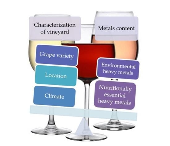
1. Introduction
- To what extent do processing methods affect the trace-element composition of wine?
- What happens to trace elements as wines age?
- How much inter-year variability is there in wines from one vineyard or region?
- (i)
- multi-element dataset is needed for fingerprinting;
- (ii)
- multivariate statistical techniques are required for data analysis; and
- (iii)
- Inductively Coupled Plasma—Mass Spectrometry (ICP-MS) is one of the most promising analytical methods for trace and ultra-trace element fingerprinting of wines, which is characterized as fast, routine and accurate.
2. Results and Discussion
2.1. Occurrence of Metals in Wine and Its Level
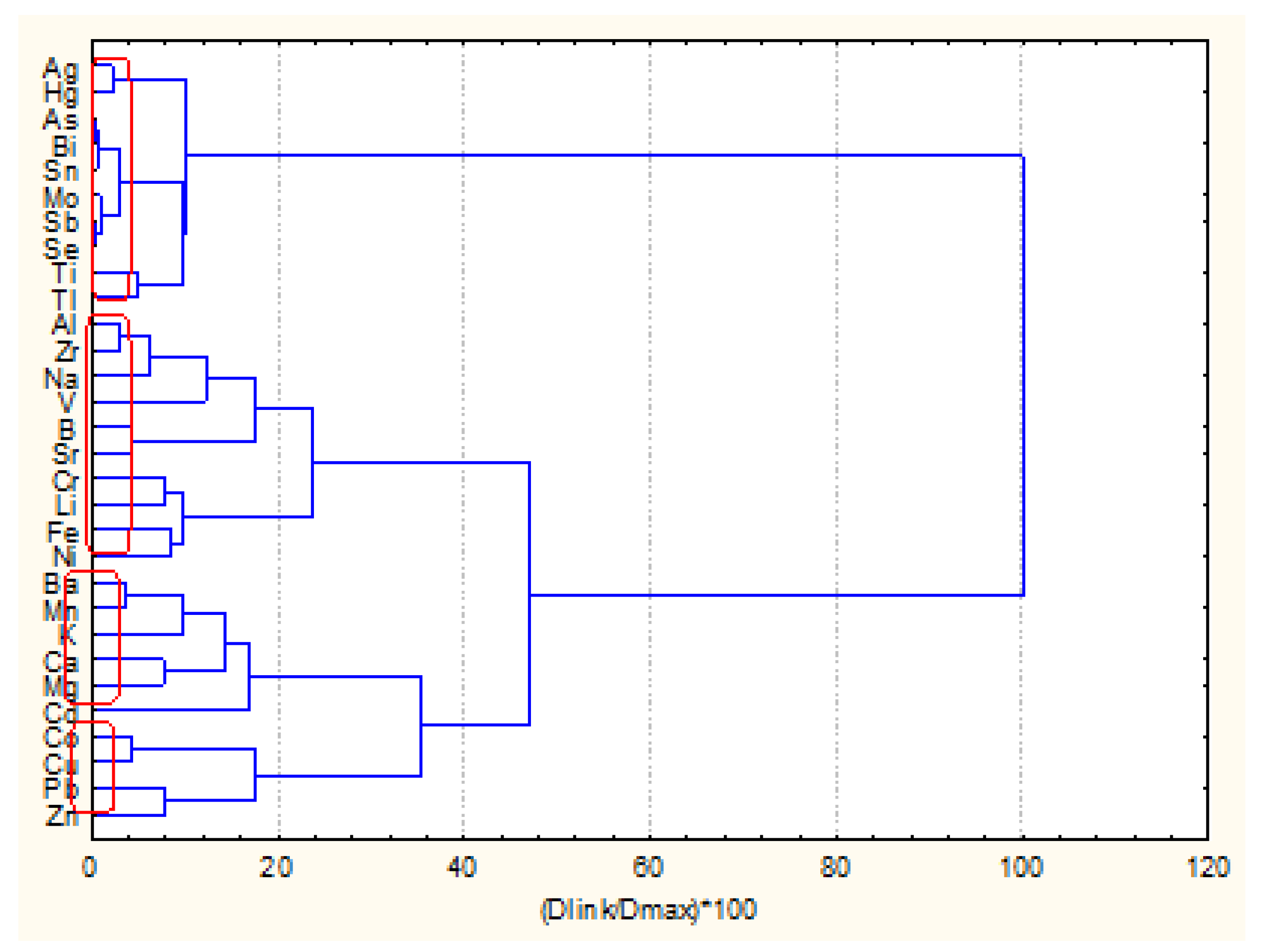
2.2. Chemometric Assessment of Multiparametric Data Set Obtained during Analysis of Wine Samples
- K1 (Zn, Pb, Cu, Co)
- K2 (Cd, Mg, Ca, K, Mn, Ba)
- K3 (Ni, Fe, Li, Cr, Sr, B, V, Na, Zr, Al)
- K4 (Tl, Ti, Se, Sb, Mo, Sn, Bi, As, Hg, Ag)
- K1 (10w, 11w, 12w, 7r, 8r, 9r, 20r)
- K2 (18w, 19w, 20w, 24w, 10r, 11r, 13r, 14r, 15r, 16r, 17r, 18r)
- K3 (2w, 3w, 4w, 5w, 6w, 7w, 8w, 9w, 13w, 14w, 15w, 16w, 17w, 21w, 22w, 23w, 1r, 2r, 3r, 4r, 5r, 6r, 12r, 19r)
3. Materials and Methods
3.1. Reagents and Standards
3.2. Samples
3.3. Equipment Used
3.4. Chemometric Analysis
4. Conclusions
Supplementary Materials
Author Contributions
Funding
Acknowledgments
Conflicts of Interest
References
- Płotka-Wasylka, J.; Rutkowska, M.; Cieślik, B.; Tyburcy, A.; Namieśnik, J. Determination of selected metals in fruit wines by spectroscopic techniques. J. Anal. Meth. Chem. 2017, 2017. [Google Scholar] [CrossRef] [PubMed]
- Goldberg, D.M.; Bromberg, I.L. Health effects of moderate alcohol consumption: A paradigmatic risk factor. Clin. Chim. Acta 1996, 246, 1–3. [Google Scholar] [CrossRef]
- Italian Office Gazette; Italian Parliament: Rome, Italy, 1987.
- Kostić, D.; Mitić, S.; Miletić, G.; Despotović, S.; Zarubica, A. The concentrations of Fe, Cu and Zn in selected wines from South-East Serbia. J. Serb. Chem. Soc. 2010, 75, 1701–1709. [Google Scholar] [CrossRef]
- Fabani, M.P.; Arrúa, R.C.; Vázquez, F.; Diaz, M.P.; Baroni, M.V.; Wunderlin, D.A. Evaluation of elemental profile coupled to chemometrics to assess the geographical origin of Argentinean wines. Food Chem. 2010, 119, 372–379. [Google Scholar] [CrossRef]
- Pyrzyńska, K. Chemical speciation and fractionation of metals in wine. Chem. Spec. Bioavailab. 2007, 19, 1–8. [Google Scholar] [CrossRef] [Green Version]
- Rousseva, M. Copper and Iron Speciation in White Wine: Impact on Wine Oxidation and Influence of Bentonite Fining and Initial Copper and Iron Juice Concentrations. Master’s Thesis, Groupe École Supérieure d’Agriculture d’Angers, Angers, France, 2014. [Google Scholar]
- Riganakos, K.A.; Veltsistas, P.G. Comparative spectrophotometric determination of the total iron content in various white and red Greek wines. Food Chem. 2003, 82, 637–643. [Google Scholar] [CrossRef]
- Monasterio, R.P.; Wuilloud, R.G. Trace level determination of cadmium in wine by on-line preconcentration in a 5-Br-PADAP functionalized wool-packed microcolumn coupled to flame atomic absorption spectrometry. Talanta 2009, 79, 1484–1488. [Google Scholar] [CrossRef] [PubMed]
- Elci, L.; Arslan, Z.; Tyson, J.F. Determinationof lead inwine and rum samples by flow injection-hydride generation-atomic absorption spectrometry. J. Hazard. Mat. 2009, 162, 880–885. [Google Scholar] [CrossRef] [PubMed]
- Greenough, J.D.; Mallory-Greenough, L.M.; Fryer, B.J. Geology and wine: Regional trace element fingerprinting of Canadian wines. Geosci. Can. 2005, 32, 129–138. [Google Scholar]
- Geana, I.; Iordache, A.; Ionete, R.; Marinescu, A.; Ranca, A.; Culea, M. Geographical origin identification of Romanian wines by ICP-MS elemental analysis. Food Chem. 2013, 138, 1125–1134. [Google Scholar] [CrossRef] [PubMed]
- Woldemariam, D.M.; Chandravanshi, B.S. Concentration levels of essential and non-essential elements in selected ethiopian wines. Bull. Chem. Soc. Ethiop. 2011, 25, 169–180. [Google Scholar] [CrossRef]
- Zioła-Frankowska, A.; Frankowski, M. Determination of selected metals in wines using inductively coupled plasma optical emission spectrometry with mini torch. Food Anal. Meth. 2017, 10, 180–190. [Google Scholar] [CrossRef]
- Massart, D.L.; Kaufman, L. The Interpretation of Analytical Chemical Data by the Use of Cluster Analysis; Elsevier: Amsterdam, The Netherlands, 1983. [Google Scholar]
Sample Availability: Samples of the compounds are Not available from the authors. |


| Country | Concentration of Metals (mg/L) | |||||||
|---|---|---|---|---|---|---|---|---|
| Al | As | Cd | Cu | Na | Pb | Ti | Zn | |
| Australia | - | 0.10 | 0.05 | 5.00 | - | 0.20 | - | 5.00 |
| Germany | 8.00 | 0.10 | 0.01 | 5.00 | - | 0.30 | 1.00 | 5.00 |
| Italy | - | - | - | 10.00 | - | 0.30 | - | 5.00 |
| Poland | - | 0.20 | 0.03 | - | - | 0.30 | - | - |
| OIV | - | 0.20 | 0.01 | 1.00 | 60 | 0.15 | - | 5.00 |
| Metal | Concentration of Metals (mg/L) in Wine of Different Origin | |||||||||
|---|---|---|---|---|---|---|---|---|---|---|
| American | Czech | Ethiopian | French | German | Greek | Hungarian | Italian | Spanish | Polish | |
| K | 462–1147 | 493–3056 | 694–767 | 265–426 | 480–1860 | 955–2089 | 489–1512 | 750–1500 | 338–2032 | 97–3250 |
| Ca | 17–94 | 40–100 | 28–37 | 65–161 | 58–200 | 14.0–47.5 | 51–164 | 30–151 | 12–241 | 32–137 |
| Mg | 100–245 | 7.8–138 | 58–79 | 55–96 | 56–105 | 82.5–122.5 | 72–174 | 53–115 | 50–236 | 42.7–161 |
| Pb | -- | 0.010–1.253 | 0.14–031 | 0.006–0.023 | -- | ND–0.62 | -- | 0.01–0.35 | 0.001–0.096 | 0.006–0.349 |
| Zn | 0.75–3.60 | -- | 1.82–2.70 | 0.44–0.74 | 0.3–1.5 | 0.05–8.9 | 0.6–1.9 | 0.135–4.8 | ND–4.63 | 0.007–2.339 |
| Cd | -- | 0.000055–0.0033 | <0.01 | ND–0.0002 | -- | ND–0.03 | 0.00014–0.54 | 0.0012–0.0016 | ND–0.019 | 0.00002–0.0025 |
| Fe | 1.2–6.6 | 0.9–5.2 | 1.42–3.16 | 0.81–2.51 | 0.4–4.2 | 0.7–7.3 | 2.03–23.7 | 1.35–27.8 | 0.4–17.4 | 0.1558–2.775 |
| Na | 7–106 | 2.0–110 | 24–25 | 7.7–14.6 | 6–25 | 5.5–150 | 18.6–81.1 | 3.4–200 | 3.5–300 | 0.005–3.823 |
| Cu | 0.05–0.58 | 0.012–6.827 | 0.5–1.5 | ND–0.48 | 0.02–0.71 | 0.2–1.65 | 0.15–2.57 | 0.001–1.34 | ND–3.1 | <0.0002–0.796 |
| Mn | 0.81–4.08 | 0.28–3.26 | 1.04–1.88 | 0.63–0.96 | 0.5–1.3 | ND–2.3 | 0.12–2.9 | 0.67–2.5 | 0.1–5.5 | 0.329–9.219 |
| Ni | -- | 0.19–0.034 | 0.18–0.25 | ND–0.052 | -- | ND–0.5 | -- | 0.015–0.21 | 0.005–0.079 | 0.00002–0.245 |
| Co | -- | ND–0.018 | ND–0.09 | 0.004-0.005 | 0.004-0.005 | ND–0.04 | 0.003–0.009 | 0.003-0.006 | ND–04 | <0.00002–0.007 |
| Cr | -- | 0.032–0.037 | ND–0.09 | 0.006-0.09 | 0.01-0.41 | ND–0.41 | 0.032–0.062 | 0.02-0.05 | 0.025–0.029 | 0.0037–0.095 |
| Type of Wine | Concentration of Metal | |||||||||||||||||||||||||||||
|---|---|---|---|---|---|---|---|---|---|---|---|---|---|---|---|---|---|---|---|---|---|---|---|---|---|---|---|---|---|---|
| Ag | Al | As | Ba | Bi | Cd | Co | Cr | Cu | Fe | Hg | Li | Mo | Na | Ni | Pb | Sb | Se | Sn | Sr | Ti | Tl | V | Zr | B | Ca | K | Mg | Mn | Zn | |
| [µg/L] | [mg/L] | |||||||||||||||||||||||||||||
| W | 1.4 | 710 | 26 | 140 | 49 | 1 | 2 | 14 | 290 | 520 | 0.4 | 5,6 | 7.4 | 890 | 64 | 20 | 2.3 | 24 | 14.1 | 290 | 33 | 0.87 | 7.5 | 5.9 | 3730 | 7461 | 91145 | 9376 | 192 | 73.4 |
| R | 0.2 | 580 | 6 | 310 | 2 | 0,6 | 2 | 12 | 130 | 790 | 0.3 | 11.2 | 3.4 | 1050 | 53 | 28 | 0.4 | 3.9 | 0.12 | 490 | 30 | 0.81 | 8.2 | 2.5 | 6870 | 7504 | 182845 | 10600 | 318 | 34.8 |
| Variable | PC1 | PC2 | PC3 | PC4 | PC5 | PC6 | PC7 | PC8 |
|---|---|---|---|---|---|---|---|---|
| Factor 1 | Factor 2 | Factor 3 | Factor 4 | Factor 5 | Factor 6 | Factor 7 | Factor 8 | |
| Ag | 0.728 | 0.030 | −0.149 | −0.007 | 0.324 | 0.048 | −0.193 | −0.153 |
| Al | −0.041 | 0.835 | −0.021 | 0.232 | 0.113 | −0.046 | 0.248 | 0.015 |
| As | 0.976 | 0.018 | 0.069 | −0.026 | 0.005 | 0.005 | 0.016 | 0.033 |
| B | −0.162 | 0.007 | 0.097 | 0.217 | −0.196 | 0.065 | 0.836 | 0.062 |
| Ba | −0.199 | 0.089 | 0.147 | −0.185 | −0.842 | 0.067 | 0.164 | −0.063 |
| Bi | 0.980 | 0.030 | 0.060 | −0.005 | 0.051 | −0.014 | −0.061 | −0.002 |
| Ca | −0.158 | −0.051 | −0.679 | 0.228 | −0.457 | 0.068 | −0.105 | −0.074 |
| Cd | 0.003 | −0.008 | 0.033 | −0.127 | −0.134 | −0.903 | −0.045 | −0.024 |
| Co | 0.032 | 0.281 | −0.837 | −0.080 | 0.197 | −0.127 | 0.193 | −0.093 |
| Cr | 0.111 | 0.033 | −0.130 | 0.856 | 0.105 | 0.021 | −0.130 | 0.079 |
| Cu | −0.032 | −0.130 | −0.852 | −0.183 | 0.107 | 0.108 | −0.087 | 0.082 |
| Fe | −0.136 | 0.176 | 0.076 | 0.646 | −0.258 | 0.232 | 0.237 | 0.154 |
| Hg | 0.733 | 0.187 | −0.319 | 0.040 | 0.386 | −0.087 | −0.256 | −0.131 |
| K | −0.290 | −0.458 | −0.042 | 0.018 | −0.508 | 0.348 | 0.307 | −0.040 |
| Li | −0.135 | 0.034 | 0.029 | 0.517 | 0.275 | 0.112 | 0.406 | 0.483 |
| Mg | −0.100 | −0.331 | −0.356 | 0.096 | −0.531 | −0.214 | 0.011 | −0.323 |
| Mn | −0.246 | −0.165 | 0.185 | −0.107 | −0.775 | −0.395 | 0.017 | 0.017 |
| Mo | 0.944 | 0.109 | 0.035 | 0.083 | 0.062 | 0.008 | −0.165 | 0.009 |
| Na | −0.045 | 0.570 | −0.055 | 0.052 | 0.243 | −0.083 | 0.627 | 0.014 |
| Ni | 0.037 | 0.104 | 0.177 | 0.638 | 0.164 | −0.028 | 0.309 | −0.043 |
| Pb | −0.041 | −0.062 | 0.006 | 0.088 | 0.007 | −0.003 | 0.016 | 0.927 |
| Sb | 0.965 | 0.112 | 0.022 | 0.033 | 0.128 | -0.008 | −0.130 | 0.033 |
| Se | 0.948 | 0.047 | 0.013 | 0.057 | 0.155 | 0.032 | −0.152 | 0.008 |
| Sn | 0.947 | −0.079 | 0.071 | −0.079 | −0.051 | 0.064 | 0.060 | 0.051 |
| Sr | −0.138 | 0.390 | −0.014 | 0.099 | −0.355 | 0.041 | 0.711 | −0.102 |
| Ti | 0.648 | 0.388 | −0.008 | 0.030 | 0.215 | −0.408 | 0.181 | −0.160 |
| Tl | 0.785 | 0.160 | 0.068 | −0.115 | 0.048 | -0.136 | 0.455 | −0.060 |
| V | 0.206 | 0.729 | 0.122 | −0.092 | −0.134 | 0.242 | −0.138 | −0.029 |
| Zn | 0.053 | −0.071 | −0.587 | 0.191 | 0.228 | 0.053 | −0.314 | 0.530 |
| Zr | 0.242 | 0.776 | −0.123 | 0.163 | 0.097 | −0.138 | 0.275 | −0.093 |
| Expl.Var % | 26.9 | 10.2 | 8.9 | 7.4 | 9.9 | 5.1 | 9.3 | 5.5 |
| Parameter and Accessories | ICP-MS | ICP-OES |
|---|---|---|
| Radio frequency power generator [kW] | 1.2 | 1.2 |
| Gas type | Argon | Argon |
| Plasma gas flow rate [L min−1] | 8.0 | 7.0 |
| Auxiliary gas flow rate [L min−1] | 1.1 | 0.6 |
| Nebulization gas flow rate [L min−1] | 0.7 | 0.7 |
| Torch | Mini-torch (quartz) | Mini-torch (quartz) |
| Nebulizer | Coaxial | Burgener NX-175 |
| Spray chamber temperature | 3 °C | Room temperature |
| Drain | Gravity fed | Gravity fed |
| Internal Standard | Automatic addition | - |
| Sampling depth | 5 mm | - |
| Collision Cell Gas flow (He) | 6 mL min−1 | - |
| Cell Voltage | −21 V | - |
| Enersgy Filter | 7.0 V | - |
| Number of replicates | 3 | 3 |
| Integration conditions/number of scans | 10 | - |
© 2018 by the authors. Licensee MDPI, Basel, Switzerland. This article is an open access article distributed under the terms and conditions of the Creative Commons Attribution (CC BY) license (http://creativecommons.org/licenses/by/4.0/).
Share and Cite
Płotka-Wasylka, J.; Frankowski, M.; Simeonov, V.; Polkowska, Ż.; Namieśnik, J. Determination of Metals Content in Wine Samples by Inductively Coupled Plasma-Mass Spectrometry. Molecules 2018, 23, 2886. https://doi.org/10.3390/molecules23112886
Płotka-Wasylka J, Frankowski M, Simeonov V, Polkowska Ż, Namieśnik J. Determination of Metals Content in Wine Samples by Inductively Coupled Plasma-Mass Spectrometry. Molecules. 2018; 23(11):2886. https://doi.org/10.3390/molecules23112886
Chicago/Turabian StylePłotka-Wasylka, Justyna, Marcin Frankowski, Vasil Simeonov, Żaneta Polkowska, and Jacek Namieśnik. 2018. "Determination of Metals Content in Wine Samples by Inductively Coupled Plasma-Mass Spectrometry" Molecules 23, no. 11: 2886. https://doi.org/10.3390/molecules23112886