
“Transitivity”: A Code for Computing Kinetic and Related Parameters in Chemical Transformations and Transport Phenomena

 ,
,
Abstract
:
1. Introduction
2. Theoretical Background
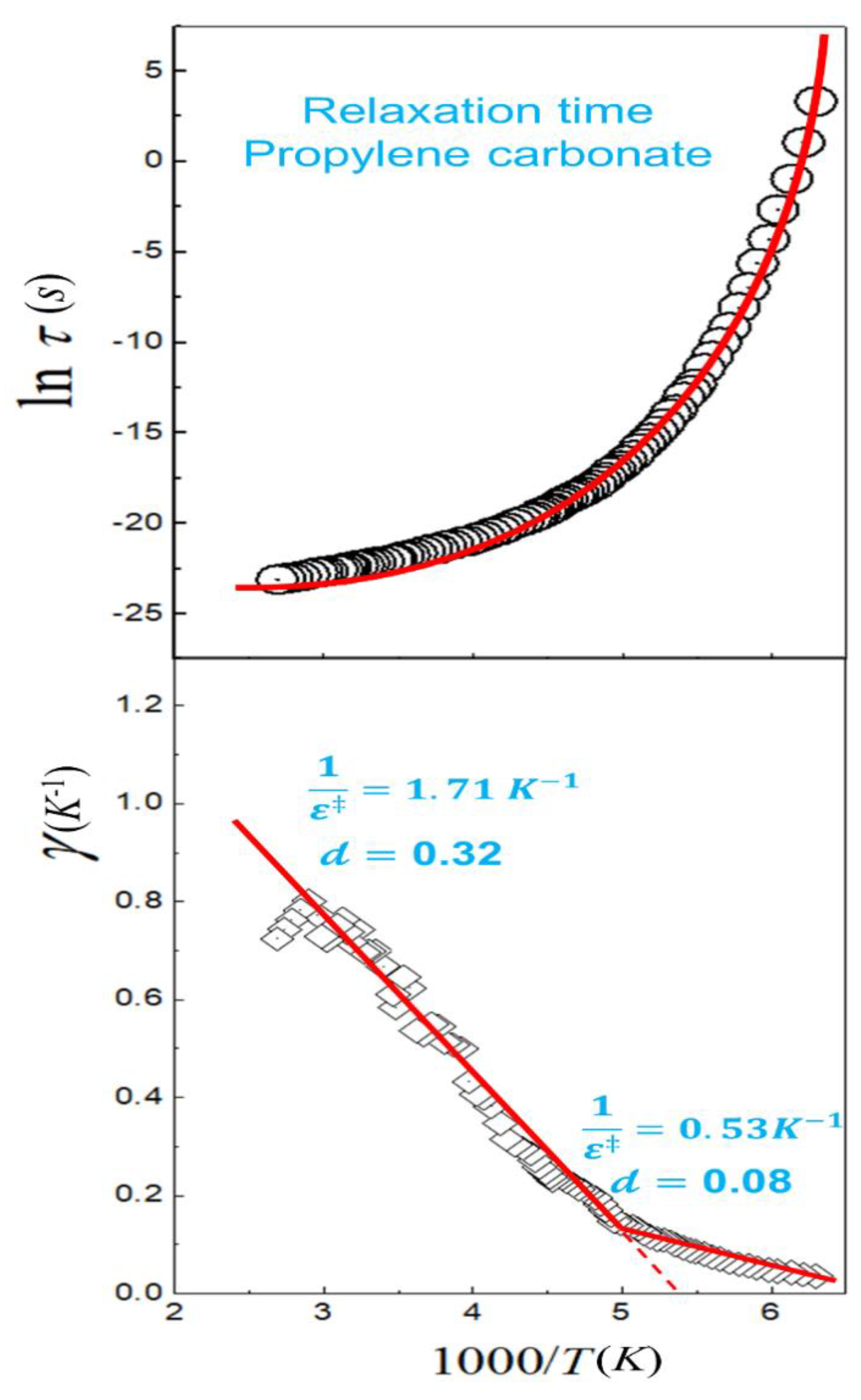
2.1. Phenomenology of Temperature Dependence of the Reaction Rate Constant
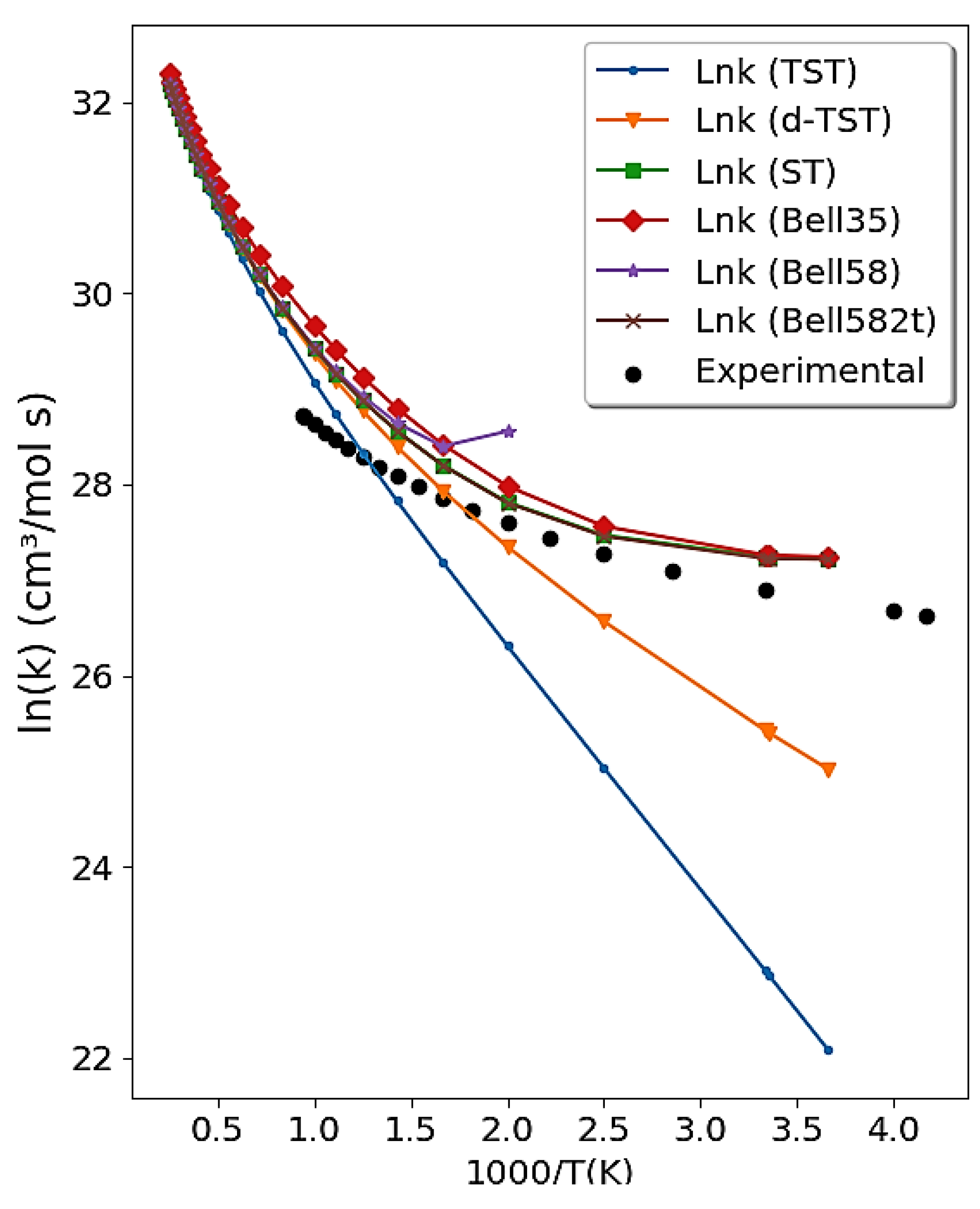
2.2. Calculation of Reaction Rate Constant
2.2.1. Deformed Transition-State Theory (-TST)
2.2.2. Bell35 and Bell58
2.2.3. Skodje and Truhlar, ST
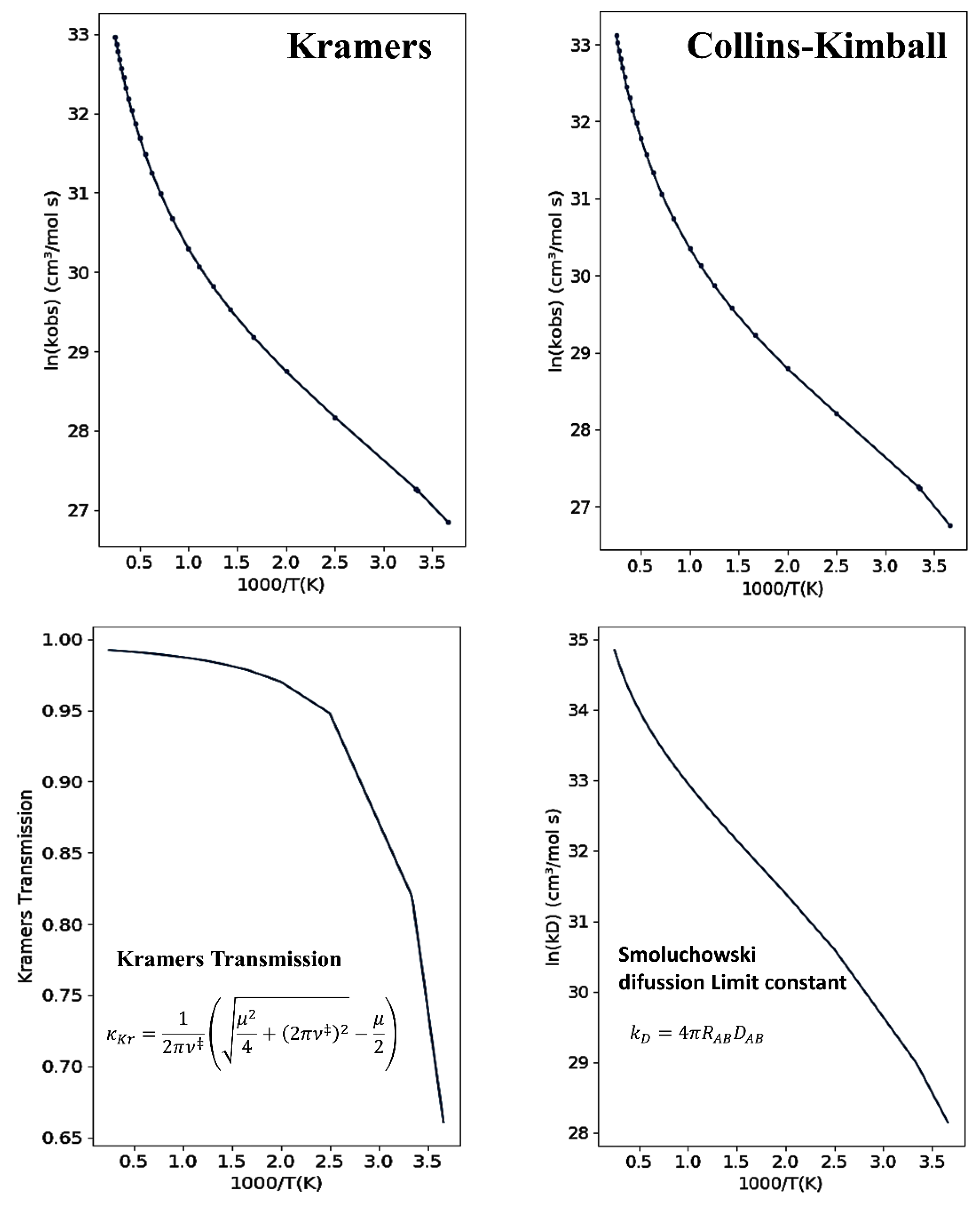
2.3. Solvent Effect on Reaction Rate Constant
2.3.1. Collins–Kimball Formulation
2.3.2. Kramers’ Formulation
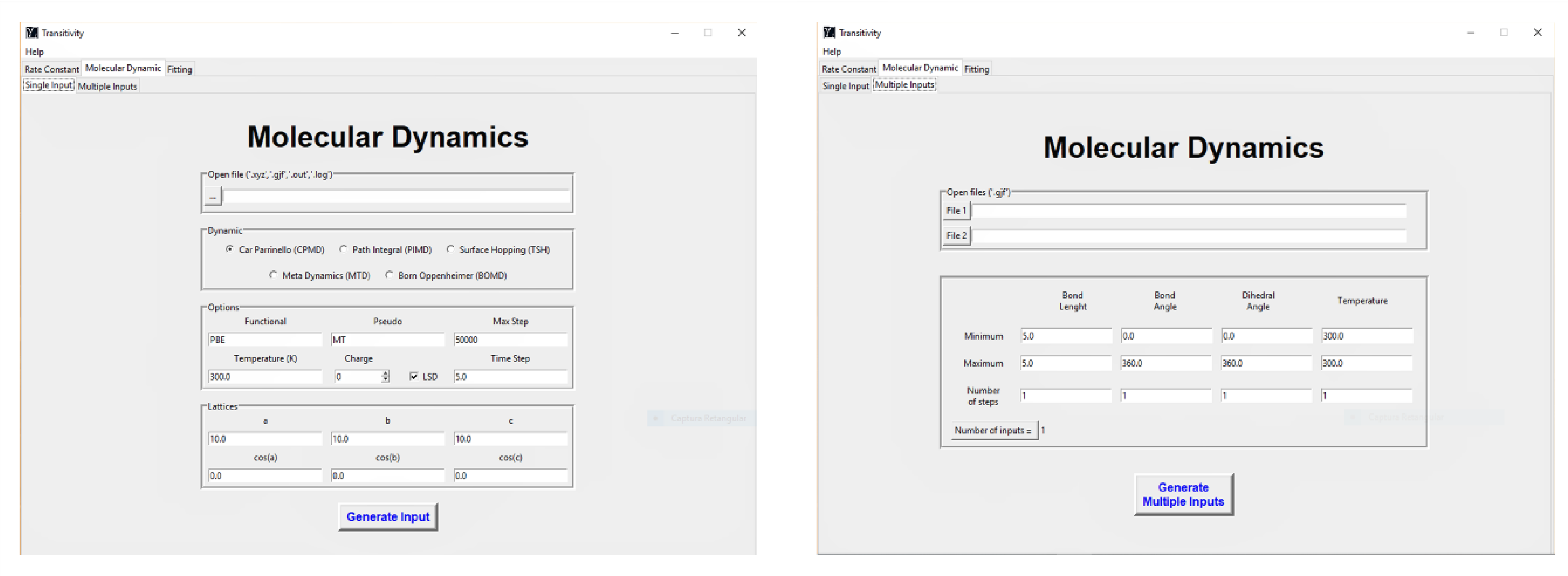
3. Handling the Transitivity Code
4. Examples
4.1. Fitting Mode—Arrhenius and Transitivity Plots
4.2. Reaction Rate Constants’ Mode
4.2.1. The OH + HCl → H2O + Cl Reaction
4.2.2. The NH3 + OH → NH2 + H2O Reaction
4.3. CPMD Input Files Generator
5. Final Remarks
- Calculation of the kinetic rate constants for chemical reactions from the potential energy surface features profile, such as the CH4 + OH [60], CH3OH + H [99], OH + HCl [44], OH + HI [43], to proton rearrangement of enol forms of curcumin [100], OH + H2 [101], and chiral nucleophilic substitution reaction [102].
Author Contributions
Funding
Acknowledgments
Conflicts of Interest
Appendix A

| Symbols | Nomenclature |
|---|---|
| Rate constant | |
| T | Temperature |
| Boltzmann constant | |
| Lagrange multiplier | |
| Transitivity function | |
| Deformed parameter | |
| Planck’s constant | |
| Partition functions | |
| AM | Aquilanti-Mundim |
| Enthalpy of reaction | |
| ASCC | Aquilanti–Sanchez–Coutinho–Carvalho |
| NTS | Nakamura–Takayanagi–Sato |
| TST | Transition-State Theory |
| GSA | Generalized Simulated Annealing |
| -TST | Deformed Transition-State Theory |
| ST | Skodje and Truhlar tunneling correction |
| Bell35 | Bell’s tunneling correction of 1935 |
| Bell58 | Bell’s tunneling correction of 1958 |
| barrier height (Eyring’s parameter) | |
| Apparent Activation Energy | |
| Energy parameter from NTS formula | |
| Energy parameter from ASCC formula | |
| B | Temperature parameter from VFT formula |
| Temperature parameter from NTS and VFT formulas. | |
| Crossover temperature | |
| Diffusion rate constant | |
| Imaginary frequency | |
| Overall reaction rate constant | |
| Transmission factor from Kramers’ model | |
| Friction constant | |
| Viscosity | |
| DFT | Density functional theory |
| BOMD | Born-Oppenheimer molecular dynamics |
| CPMD | Car-Parrinello molecular dynamics |
| PIMD | Path-Integral molecular dynamics |
| MTD | Metadynamics |
| TSH | Trajectory Surface Hopping |
References
- Valter Henrique, C.-S.; Coutinho, N.D.; Aquilanti, V. From the Kinetic Theory of Gases to the Kinetics of Chemical Reactions: On the Verge of the Thermodynamical and the Kinetic Limits. Molecules 2019. to be submitted. [Google Scholar]
- Aquilanti, V.; Coutinho, N.D.; Carvalho-Silva, V.H. Kinetics of Low-Temperature Transitions and Reaction Rate Theory from Non-Equilibrium Distributions. Philos. Trans. R. Soc. London A 2017, 375, 20160204. [Google Scholar] [CrossRef]
- Aquilanti, V.; Borges, E.P.; Coutinho, N.D.; Mundim, K.C.; Carvalho-Silva, V.H. From statistical thermodynamics to molecular kinetics: the change, the chance and the choice. Rend. Lincei. Sci. Fis. e Nat. 2018, 28, 787–802. [Google Scholar] [CrossRef]
- Gentili, P.L. The fuzziness of the molecular world and its perspectives. Molecules 2018, 23, 2074. [Google Scholar] [CrossRef]
- Gentili, P.L. Untangling Complex Systems: A Grand Challenge for Science; CRC Press: Boca Raton, FL, USA, 2018; ISBN 9780429847547. [Google Scholar]
- Atkinson, R. Kinetics and mechanisms of the gas-phase reactions of the hydroxyl radical with organic compounds under atmospheric conditions. Chem. Rev. 1986, 86, 69–201. [Google Scholar] [CrossRef]
- Limbach, H.-H.; Miguel Lopez, J.; Kohen, A. Arrhenius curves of hydrogen transfers: tunnel effects, isotope effects and effects of pre-equilibria. Philos. Trans. R. Soc. B Biol. Sci. 2006, 361, 1399–1415. [Google Scholar] [CrossRef] [Green Version]
- Smith, I.W.M. The temperature-dependence of elementary reaction rates: Beyond Arrhenius. Chem. Soc. Rev. 2008, 37, 812–826. [Google Scholar] [CrossRef]
- Sims, I.R. Low-temperature reactions: Tunnelling in space. Nat. Chem. 2013, 5, 734–736. [Google Scholar] [CrossRef] [PubMed]
- Peleg, M.; Normand, M.D.; Corradini, M.G. The Arrhenius Equation Revisited. Crit. Rev. Food Sci. Nutr. 2012, 52, 830–851. [Google Scholar] [CrossRef] [PubMed]
- Darrington, R.T.; Jiao, J. Rapid and Accurate Prediction of Degradant Formation Rates in Pharmaceutical Formulations Using High-Performance Liquid Chromatography-Mass Spectrometry. J. Pharm. Sci. 2004, 93, 838–846. [Google Scholar] [CrossRef]
- Giordano, D.; Russell, J.K. Towards a structural model for the viscosity of geological melts. Earth Planet. Sci. Lett. 2018, 501, 202–212. [Google Scholar] [CrossRef]
- Klinman, J.P.; Kohen, A. Hydrogen Tunneling Links Protein Dynamics to Enzyme Catalysis. Annu. Rev. Biochem. 2013, 82, 471–496. [Google Scholar] [CrossRef] [Green Version]
- Warshel, A.; Bora, R.P. Perspective: Defining and quantifying the role of dynamics in enzyme catalysis. J. Chem. Phys. 2016, 144, 180901. [Google Scholar] [CrossRef]
- Laidler, K.J. A Glossary of Terms Used in Chemical Kinetics, Including Reaction Dynamics. Pure Appl. Chem. 1996, 68, 149–192. [Google Scholar] [CrossRef]
- Tolman, R.C. Statistical Mechanics Applied to Chemical Kinetics. J. Amer. Chem. Soc. 1920, 42, 2506–2528. [Google Scholar] [CrossRef]
- Glasstone, S.; Laidler, K.J.; Eyring, H. The Theory of Rate Processes: The Kinetics of Chemical Reactions, Viscosity, Diffusion and Electrochemical Phenomena; International chemical series; McGraw-Hill: New York, NY, USA, 1941. [Google Scholar]
- Truhlar, D.G. Current Status of Transition-State Theory. J. Phys. Chem. 1983, 2664–2682. [Google Scholar] [CrossRef]
- Kooij, D.M. Über die Zersetzung des gasförmigen Phosphorwasserstoffs. Zeitschrift für Phys. Chemie 1893, 12, 155–161. [Google Scholar]
- Bělehrádek, J. A unified theory of cellular rate processes based upon an analysis of temperature action. Protoplasma 1957, 48, 53–71. [Google Scholar] [CrossRef]
- Vogel, H. Das temperature-abhangigketsgesetz der viskositat von flussigkeiten. Phys. Z 1921, 22, 645–646. [Google Scholar]
- Fulcher, G.S. Analysis of Recent Measurements of the Viscosity of Glasses. J. Am. Ceram. Soc. 1925, 8, 339–355. [Google Scholar] [CrossRef]
- Tammann, G.; Hesse, W. Die Abhängigkeit der Viscosität von der Temperatur bie unterkühlten Flüssigkeiten. Zeitschrift für Anorg. und Allg. Chemie 1926, 156, 245–257. [Google Scholar] [CrossRef]
- Nakamura, K.; Takayanagi, T.; Sato, S. A modified arrhenius equation. Chem. Phys. Lett. 1989, 160, 295–298. [Google Scholar] [CrossRef]
- Aquilanti, V.; Mundim, K.C.; Elango, M.; Kleijn, S.; Kasai, T. Temperature dependence of chemical and biophysical rate processes: Phenomenological approach to deviations from Arrhenius law. Chem. Phys. Lett. 2010, 498, 209–213. [Google Scholar] [CrossRef]
- Coutinho, N.D.; Silva, Y.S.; de Fazio, D.; Cavalli, S.; Carvalho-Silva, V.H.; Aquilanti, V. Chemical Kinetics under Extreme Conditions: Exact, Phenomenological and First-Principles Computational Approaches. In The Astrochemical Observatory: Focus on Chiral Molecules; Accademia Nazionale delle Scienze detta dei XL: Rome, Italy, 2018; pp. 1–15. [Google Scholar]
- Carvalho-Silva, V.H.; Coutinho, N.D.; Aquilanti, V. Temperature dependence of rate processes beyond Arrhenius and Eyring: Activation and Transitivity. Front. Chem. 2019, 7, 380. [Google Scholar] [CrossRef] [PubMed]
- Fernandez-Ramos, A.; Ellingson, B.A.; Garrett, B.C.; Truhlar, D.G. Variational Transition State Theory with Multidimensional Tunneling. In Reviews in Computational Chemistry; John Wiley & Sons, Inc.: Hoboken, NJ, USA, 2007; pp. 125–232. ISBN 9780470116449. [Google Scholar]
- Marcus, R.A. Electron transfer reactions in chemistry. Theory and experiment. Rev. Mod. Phys. 1993, 65, 599–610. [Google Scholar] [CrossRef] [Green Version]
- Miller, W. Quantum mechanical transition state theory and a new semiclassical model for reaction rate constants. J. Chem. Phys. 1974, 61, 1823. [Google Scholar] [CrossRef]
- Richardson, J.O. Ring-Polymer Approaches to Instanton Theory. Ph.D. Thesis, University of Cambridge, Cambridge, UK, 2012. [Google Scholar]
- Zhang, Y.; Stecher, T.; Cvitaš, M.T.; Althorpe, S.C. Which Is Better at Predicting Quantum-Tunneling Rates: Quantum Transition-State Theory or Free-Energy Instanton Theory? J. Phys. Chem. Lett. 2014, 5, 3976–3980. [Google Scholar] [CrossRef]
- Xiao, R.; Gao, L.; Wei, Z.; Spinney, R.; Luo, S.; Wang, D.; Dionysiou, D.D.; Tang, C.J.; Yang, W. Mechanistic insight into degradation of endocrine disrupting chemical by hydroxyl radical: An experimental and theoretical approach. Environ. Pollut. 2017, 231, 1446–1452. [Google Scholar] [CrossRef]
- Luo, S.; Gao, L.; Wei, Z.; Spinney, R.; Dionysiou, D.D.; Hu, W.P.; Chai, L.; Xiao, R. Kinetic and mechanistic aspects of hydroxyl radical‒mediated degradation of naproxen and reaction intermediates. Water Res. 2018, 137, 233–241. [Google Scholar] [CrossRef]
- Gao, Y.; Ji, Y.; Li, G.; An, T. Mechanism, kinetics and toxicity assessment of OH-initiated transformation of triclosan in aquatic environments. Water Res. 2014, 49, 360–370. [Google Scholar] [CrossRef]
- De Sainte Claire, P. Degradation of PEO in the solid state: A theoretical kinetic model. Macromolecules 2009, 42, 3469–3482. [Google Scholar] [CrossRef]
- Ahubelem, N.; Shah, K.; Moghtaderi, B.; Page, A.J. Formation of benzofuran and chlorobenzofuran from 1,3-dichloropropene: A quantum chemical investigation. Int. J. Quantum Chem. 2015, 115, 1739–1745. [Google Scholar] [CrossRef]
- Zavala-Oseguera, C.; Galano, A.; Merino, G. Computational study on the kinetics and mechanism of the carbaryl + OH reaction. J. Phys. Chem. A 2014, 118, 7776–7781. [Google Scholar] [CrossRef] [PubMed]
- Döntgen, M.; Przybylski-Freund, M.-D.; Kröger, L.C.; Kopp, W.A.; Ismail, A.E.; Leonhard, K. Automated discovery of reaction pathways, rate constants, and transition states using reactive molecular dynamics simulations. J. Chem. Theory Comput. 2015, 11, 2517–2524. [Google Scholar] [CrossRef] [PubMed]
- Piccini, G.; McCarty, J.; Valsson, O.; Parrinell, M. Variational Flooding Study of a S2 Reaction. J. Phys. Chem. A 2017, 8, 580–583. [Google Scholar]
- Fleming, K.L.; Tiwary, P.; Pfaendtner, J. New Approach for Investigating Reaction Dynamics and Rates with Ab Initio Calculations. J. Phys. Chem. A 2016, 120, 299–305. [Google Scholar] [CrossRef] [PubMed]
- Lancar, I.T.; Mellouki, A.; Poulet, G. Kinetics of the reactions of hydrogen iodide with hydroxyl and nitrate radicals. Chem. Phys. Lett. 1991, 177, 554–558. [Google Scholar] [CrossRef]
- Coutinho, N.D.; Carvalho-Silva, V.H.; de Oliveira, H.C.B.; Aquilanti, V. The HI + OH → H2O + I Reaction by First-Principles Molecular Dynamics: Stereodirectional and Anti-Arrhenius Kinetics, 2017; Volume 10408 LNCS, ISBN 9783319624037.
- Coutinho, N.D.; Sanches-Neto, F.O.; Carvalho-Silva, V.H.; de Oliveira, H.C.B.; Ribeiro, L.A.; Aquilanti, V. Kinetics of the OH+HCl→H2O+Cl reaction: Rate determining roles of stereodynamics and roaming and of quantum tunneling. J. Comput. Chem. 2018, 39, 2508–2516. [Google Scholar] [CrossRef] [PubMed]
- Isaacson, A.D.; Truhlar, D.G.; Rai, S.N.; Steckler, R.; Hancock, G.C.; Garrett, B.C.; Redmon, M.J. POLYRATE: A general computer program for variational transition state theory and semiclassical tunneling calculations of chemical reaction rates. Comput. Phys. Commun. 1987, 47, 91–102. [Google Scholar] [CrossRef]
- Duncan, W.T.; Bell, R.L.; Truong, T.N. TheRate: Program forab initio direct dynamics calculations of thermal and vibrational-state-selected rate constants. J. Comput. Chem. 1998, 19, 1039–1052. [Google Scholar] [CrossRef]
- Barker, J.R. Multiple-Well, multiple-path unimolecular reaction systems. I. MultiWell computer program suite. Int. J. Chem. Kinet. 2001, 33, 232–245. [Google Scholar] [CrossRef] [Green Version]
- Ghysels, A.; Verstraelen, T.; Hemelsoet, K.; Waroquier, M.; Van Speybroeck, V. TAMkin: A versatile package for vibrational analysis and chemical kinetics. J. Chem. Inf. Model. 2010, 50, 1736–1750. [Google Scholar] [CrossRef] [PubMed]
- Glowacki, D.R.; Liang, C.-H.; Morley, C.; Pilling, M.J.; Robertson, S.H. MESMER: An Open-Source Master Equation Solver for Multi-Energy Well Reactions. J. Phys. Chem. A 2012, 116, 9545–9560. [Google Scholar] [CrossRef] [PubMed]
- Gao, C.W.; Allen, J.W.; Green, W.H.; West, R.H. Reaction Mechanism Generator: Automatic construction of chemical kinetic mechanisms. Comput. Phys. Commun. 2016, 203, 212–225. [Google Scholar] [CrossRef] [Green Version]
- Euclides, H.O.; Barreto, P.R. APUAMA: a software tool for reaction rate calculations. J. Mol. Model. 2017, 23, 176. [Google Scholar] [CrossRef] [PubMed] [Green Version]
- Canneaux, S.; Bohr, F.; Henon, E. KiSThelP: A program to predict thermodynamic properties and rate constants from quantum chemistry results. J. Comput. Chem. 2014, 35, 82–93. [Google Scholar] [CrossRef] [PubMed]
- Coppola, C.M. Mher V Kazandjian; Matrix formulation of the energy exchange problem of multi-level systems and the code FRIGUS. Rend. Lincei Sci. Fis. e Nat. 2019, in press. [Google Scholar]
- Dzib, E.; Cabellos, J.L.; Ortíz-Chi, F.; Pan, S.; Galano, A.; Merino, G. Eyringpy: A program for computing rate constants in the gas phase and in solution. Int. J. Quantum Chem. 2018, 119, 11–13. [Google Scholar] [CrossRef]
- Mundim, K.C.; Tsallis, C. Geometry optimization and conformational analysis through generalized simulated annealing. Int. J. Quantum Chem. 1998, 58, 373–381. [Google Scholar] [CrossRef]
- Sato, S. Tunneling in bimolecular reactions. Chem. Phys. 2005, 315, 65–75. [Google Scholar] [CrossRef]
- Bell, R.P. Quantum Mechanical Effects in Reactions Involving Hydrogen. Proc. R. Soc. London. Ser. A, Math. Phys. Sci. 1935, CXLVIII.A, 241–250. [Google Scholar]
- Bell, R.P. The Tunnel Effect Correction For Parabolic Potential Barriers. Faraday Soc. Contrib. 1958, 1–4. [Google Scholar] [CrossRef]
- Skodje, R.T.; Truhlar, D.G. Parabolic tunneling calculations. J. Phys. Chem. 1981, 85, 624–628. [Google Scholar] [CrossRef]
- Carvalho-Silva, V.H.; Aquilanti, V.; de Oliveira, H.C.B.; Mundim, K.C. Deformed transition-state theory: Deviation from Arrhenius behavior and application to bimolecular hydrogen transfer reaction rates in the tunneling regime. J. Comput. Chem. 2017, 38, 178–188. [Google Scholar] [CrossRef] [PubMed]
- Collins, F.C.; Kimball, G.E. Diffusion-controlled reaction rates. J. Colloid Sci. 1949, 4, 425–437. [Google Scholar] [CrossRef]
- Kramers, H.A. Brownian motion in a field of force and the diffusion model of chemical reactions. Phys. 1940, 7, 284–304. [Google Scholar] [CrossRef]
- CPMDversion 3.17.1; CPMD, version 4.; CPMDversion 4.1; CPMDversion 3.17.1 Copyright IBM 2012.
- Claudino, D.; Gargano, R.; Carvalho-Silva, V.H.; E Silva, G.M.; Da Cunha, W.F. Investigation of the Abstraction and Dissociation Mechanism in the Nitrogen Trifluoride Channels: Combined Post-Hartree-Fock and Transition State Theory Approaches. J. Phys. Chem. A 2016, 120, 5464–5473. [Google Scholar] [CrossRef]
- Cavalli, S.; Aquilanti, V.; Mundim, K.C.; De Fazio, D. Theoretical reaction kinetics astride the transition between moderate and deep tunneling regimes: The F + HD case. J. Phys. Chem. A 2014, 118, 6632–6641. [Google Scholar] [CrossRef]
- Bell, R.P. The Tunnel Effect in Chemistry; Champman and Hall: London, UK, 1980. [Google Scholar]
- Christov, S.G. The Characteristic (Crossover) Temperature in the Theory of Thermally Activated Tunneling Processes. Mol. Eng. 1997, 7, 109–147. [Google Scholar] [CrossRef]
- Onsager, L. Electric Moments of Molecules in Liquids. J. Am. Chem. Soc. 1936, 58, 1486–1493. [Google Scholar] [CrossRef]
- Wong, M.W.; Wiberg, K.B.; Frisch, M.J. Solvent effects. 3. Tautomeric equilibria of formamide and 2-pyridone in the gas phase and solution: an ab initio SCRF study. J. Am. Chem. Soc. 1992, 114, 1645–1652. [Google Scholar] [CrossRef]
- Henriksen, N.E.; Hansen, F.Y. Theories of Molecular Reaction Dynamics: The Microscopic Foundation of Chemical Kinetics; Oxford University Press: New York, NY, USA, 2008; ISBN 9780191708251. [Google Scholar]
- Smoluchowski, M.V. Drei Vortrage uber Diffusion, Brownsche Bewegung und Koagulation von Kolloidteilchen. Phys. Zeit. 1916, 17, 557–585. [Google Scholar]
- Collins, F.C.; Kimball, G.E. Diffusion-Controlled Reactions in Liquid Solutions. Ind. Eng. Chem. 1949, 41, 2551–2553. [Google Scholar] [CrossRef]
- Eigen, M. Acid-Base Catalysis, and Enzymatic Hydrolysis. Part I: Elementary Processes. Angew. Chemie Int. Ed. English 1964, 3, 1–19. [Google Scholar] [CrossRef]
- Hallett, J. The Temperature Dependence of the Viscosity of Supercooled Water. Proc. Phys. Soc. 1963, 82, 1046–1050. [Google Scholar] [CrossRef]
- Savitzky, A.; Golay, M.J.E. Smoothing and Differentiation of Data by Simplified Least Squares Procedures. Anal. Chem. 1964, 36, 1627–1639. [Google Scholar] [CrossRef]
- Ravishankara, A.R.; Nicovich, J.M.; Thompson, R.L.; Tully, F.P. Kinetic study of the reaction of hydroxyl with hydrogen and deuterium from 250 to 1050 K. J. Phys. Chem. 1981, 85, 2498–2503. [Google Scholar] [CrossRef]
- Kohen, A.; Cannio, R.; Bartolucci, S.; Klinman, J.P. Enzyme dynamics and hydrogen tunnelling in a thermophilic alcohol dehydrogenase. Nature 1999, 399, 496–499. [Google Scholar] [CrossRef]
- Liang, Z.X.; Tsigos, I.; Bouriotis, V.; Klinman, J.P. Impact of protein flexibility on hydride-transfer parameters in thermophilic and psychrophilic alcohol dehydrogenases. J. Am. Chem. Soc. 2004, 126, 9500–9501. [Google Scholar] [CrossRef]
- Truhlar, D.; Kohen, A. Convex Arrhenius plots and their interpretation. Proc. Nat. Acad. Sci. USA 2001, 98, 848–851. [Google Scholar] [CrossRef] [Green Version]
- Coutinho, N.D.; Aquilanti, V.; Silva, V.H.C.; Camargo, A.J.; Mundim, K.C.; De Oliveira, H.C.B. Stereodirectional Origin of anti-Arrhenius Kinetics for a Tetraatomic Hydrogen Exchange Reaction: Born-Oppenheimer Molecular Dynamics for OH + HBr. J. Phys. Chem. A 2016, 120, 5408–5417. [Google Scholar] [CrossRef] [PubMed]
- de Oliveira-Filho, A.G.S.; Ornellas, F.R.; Bowman, J.M. Quasiclassical Trajectory Calculations of the Rate Constant of the OH + HBr → Br + H2O Reaction Using a Full-Dimensional Ab Initio Potential Energy Surface Over the Temperature Range 5 to 500 K. J. Phys. Chem. Lett. 2014, 5, 706–712. [Google Scholar] [CrossRef] [PubMed]
- Coutinho, N.D.; Silva, V.H.C.; de Oliveira, H.C.B.; Camargo, A.J.; Mundim, K.C.; Aquilanti, V. Stereodynamical Origin of Anti-Arrhenius Kinetics: Negative Activation Energy and Roaming for a Four-Atom Reaction. J. Phys. Chem. Lett. 2015, 6, 1553–1558. [Google Scholar] [CrossRef] [PubMed]
- Zuniga-Hansen, N.; Silbert, L.E.; Calbi, M.M. Breakdown of kinetic compensation effect in physical desorption. Phys. Rev. E 2018, 98, 032128. [Google Scholar] [CrossRef] [Green Version]
- Sims, I.R.; Smith, I.W.M.; Clary, D.C.; Bocherel, P.; Rowe, B.R. Ultra-low Temperature Kinetics of Neutral-neutral Reactions - New Experimental and Theoretical Results For OH + HBr Between 295 K and 23 K. J. Chem. Phys. 1994, 101, 1748–1751. [Google Scholar] [CrossRef]
- Souletie, J.; Tholence, J.L. Critical slowing down in spin glasses and other glasses: Fulcher versus power law. Phys. Rev. B 1985, 32, 516. [Google Scholar] [CrossRef]
- Stickel, F.; Fischer, E.W.; Richert, R. Dynamics of glass-forming liquids. II. Detailed comparison of dielectric relaxation, de-conductivity, and viscosity data. J. Chem. Phys. 1996, 104, 2043. [Google Scholar] [CrossRef]
- Drozd-Rzoska, A. Universal behavior of the apparent fragility in ultraslow glass forming systems. Sci. Rep. 2019, 9, 6816. [Google Scholar] [CrossRef]
- Silva, V.H.C.; Aquilanti, V.; de Oliveira, H.C.B.; Mundim, K.C. Uniform description of non-Arrhenius temperature dependence of reaction rates, and a heuristic criterion for quantum tunneling vs classical non-extensive distribution. Chem. Phys. Lett. 2013, 590, 201–207. [Google Scholar] [CrossRef] [Green Version]
- Frisch, M.J.; Trucks, G.W.; Schlegel, H.B.; Scuseria, G.E.; Robb, M.A.; Cheeseman, J.R.; Scalmani, G.; Barone, V.; Mennucci, B.; Petersson, G.A.; et al. Gaussian09 Revision D.01 2009; Gaussian, Inc.: Wallingford, CT, USA, 2009. [Google Scholar]
- Ravishankara, A.R.; Wine, P.H.; Wells, J.R.; Thompson, R.L. Kinetic study of the reaction of OH with HCl from 240 to 1055 K. Chem. Phys. Lett. 1985, 17, 1281–1297. [Google Scholar] [CrossRef]
- Hickel, B.; Sehested, K. Reaction of hydroxyl radicals with ammonia in liquid water at elevated temperatures. Int. J. Radiat. Appl. Instrum. Part C. Radiat. Phys. Chem. 1992, 39, 355–357. [Google Scholar] [CrossRef]
- Men’kin, V.B.; Makarov, I.E.; Pikaev, A.K. Pulse radiolysis study of reaction rates of OH and O-radicals with ammonia in aqueous solutions. High Energy Chem. (Engl. Transl.) 1989, 22, 333–336. [Google Scholar]
- Neta, P.; Maruthamuthu, P.; Carton, P.M.; Fessenden, R.W. Formation and reactivity of the amino radical. J. Phys. Chem. 1978, 82, 1875–1878. [Google Scholar] [CrossRef]
- Aquilanti, V.; Mundim, K.C.; Cavalli, S.; De Fazio, D.; Aguilar, A.; Lucas, J.M. Exact activation energies and phenomenological description of quantum tunneling for model potential energy surfaces. The F+H2 reaction at low temperature. Chem. Phys. 2012, 398, 186–191. [Google Scholar] [CrossRef]
- Rampino, S.; Pastore, M.; Garcia, E.; Pacifici, L.; Laganà, A. On the temperature dependence of the rate coefficient of formation of C2+ from C + CH+. Mon. Not. R. Astron. Soc. 2016, 460, 2368–2375. [Google Scholar] [CrossRef]
- Coutinho, N.D.; Silva, V.H.C.; Mundim, K.C.; de Oliveira, H.C.B. Description of the effect of temperature on food systems using the deformed Arrhenius rate law: deviations from linearity in logarithmic plots vs. inverse temperature. Rend. Lincei 2015, 26, 141–149. [Google Scholar] [CrossRef]
- Capitelli, M.; Pietanza, L.D. Past and present aspects of Italian plasma chemistry. Rend. Lincei. Sci. Fis. e Nat. 2019. [Google Scholar] [CrossRef]
- Agreda, N.J.L. Aquilanti–Mundim deformed Arrhenius model in solid-state reactions: Theoretical evaluation using DSC experimental data. J. Therm. Anal. Calorim. 2016, 126, 1175–1184. [Google Scholar] [CrossRef]
- Sanches-Neto, F.O.; Coutinho, N.D.; Silva, V. A novel assessment of the role of the methyl radical and water formation channel in the CH3OH + H reaction. Phys. Chem. Chem. Phys. 2017, 19, 24467–24477. [Google Scholar] [CrossRef] [PubMed]
- Santin, L.G.; Toledo, E.M.; Carvalho-Silva, V.H.; Camargo, A.J.; Gargano, R.; Oliveira, S.S. Methanol Solvation Effect on the Proton Rearrangement of Curcumin’s Enol Forms: An Ab Initio Molecular Dynamics and Electronic Structure Viewpoint. J. Phys. Chem. C 2016, 120, 19923–19931. [Google Scholar] [CrossRef]
- Carvalho-Silva, V.H.; Vaz, E.C.; Coutinho, N.D.; Kobayashi, H.; Kobayashi, Y.; Kasai, T.; Palazzetti, F.; Lombardi, A.; Aquilanti, V. The Increase of the Reactivity of Molecular Hydrogen with Hydroxyl Radical from the Gas Phase versus an Aqueous Environment: Quantum Chemistry and Transition State-Theory Calculations. In Lecture Notes in Computer Science; Springer: Cham, Switzerland, 2019; pp. 450–459. [Google Scholar]
- Rezende, M.V.C.S.; Coutinho, N.D.; Palazzetti, F.; Lombardi, A.; Carvalho-Silva, V.H. Nucleophilic substitution vs elimination reaction of bisulfide ions with substituted methanes: exploration of chiral selectivity by stereodirectional first-principles dynamics and transition state theory. J. Mol. Model. 2019, 25, 227. [Google Scholar] [CrossRef] [PubMed]
Sample Availability: Not available. |


| Formula | Chemical Processes | ||||
|---|---|---|---|---|---|
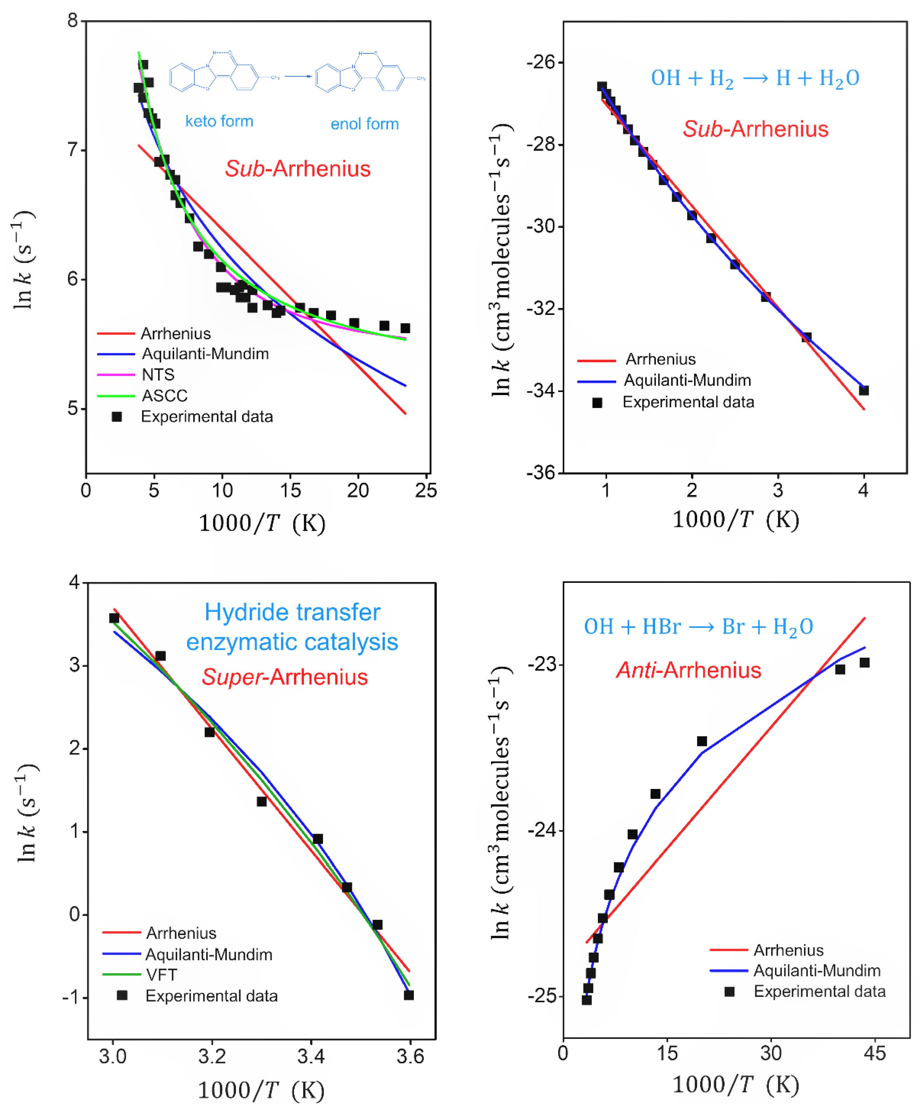
| Fitted Parameters | Keto-enol Tautomerization [7] Sub -Arrhenius (Deep-Tunneling) | OH + H2 → H + H2 [76] Sub-Arrhenius (Moderate Tunneling) | Enzymatic Catalysis [78] Super-Arrhenius | OH + HBr → Br + H2O [84] Anti-Arrhenius | |
| Arrhenius | 1.74 × 10³ | 2.1610-11 | 1.52 × 10¹¹ | 1.66 × 10⁻¹¹ | |
| 214 | 4891 | 14600 | −94.6 | ||
| 1.10 × 10⁻² | 4.2010-3 | 2.60 × 10⁻² | 6.69 × 10⁻² | ||
| Aquilanti–Mundim (AM) | 3.32 × 10⁶ | 1.1110-10 | 1.91 × 10⁴ | 7.43 × 10⁻¹⁴ | |
| 318.06 | 9170 | 2391 | −324.61 | ||
| −0.81 | −0.086 | 0.207 | 1.24 | ||
| 3.68 × 10⁻² | 6.8010-4 | 2.91 × 10⁻² | 2.78 × 10⁻³ | ||
| Aquilanti–Sanchez–Coutinho–Carvalho (ASCC) , | 2.33 × 10⁴ | - | - | - | |
| 2441 | - | - | - | ||
| 429 | - | - | - | ||
| 2.18 × 10⁻² | - | - | - | ||
| Sato–Nakamura–Takayanagi (NTS) | 3.12 × 10⁴ | - | - | - | |
| 1655 | - | - | - | ||
| 168 | - | - | - | ||
| 7.38 × 10⁻³ | - | - | - | ||
| Vogel–Fulcher–Tammann (VFT) | - | - | 1.25 × 10⁵ | - | |
| - | - | −1298 | - | ||
| - | - | 175 | - | ||
| - | - | 2.16 × 10⁻² | - |
© 2019 by the authors. Licensee MDPI, Basel, Switzerland. This article is an open access article distributed under the terms and conditions of the Creative Commons Attribution (CC BY) license (http://creativecommons.org/licenses/by/4.0/).
Share and Cite
Machado, H.G.; Sanches-Neto, F.O.; Coutinho, N.D.; Mundim, K.C.; Palazzetti, F.; Carvalho-Silva, V.H. “Transitivity”: A Code for Computing Kinetic and Related Parameters in Chemical Transformations and Transport Phenomena. Molecules 2019, 24, 3478. https://doi.org/10.3390/molecules24193478
Machado HG, Sanches-Neto FO, Coutinho ND, Mundim KC, Palazzetti F, Carvalho-Silva VH. “Transitivity”: A Code for Computing Kinetic and Related Parameters in Chemical Transformations and Transport Phenomena. Molecules. 2019; 24(19):3478. https://doi.org/10.3390/molecules24193478
Chicago/Turabian StyleMachado, Hugo G., Flávio O. Sanches-Neto, Nayara D. Coutinho, Kleber C. Mundim, Federico Palazzetti, and Valter H. Carvalho-Silva. 2019. "“Transitivity”: A Code for Computing Kinetic and Related Parameters in Chemical Transformations and Transport Phenomena" Molecules 24, no. 19: 3478. https://doi.org/10.3390/molecules24193478