
From the Kinetic Theory of Gases to the Kinetics of Rate Processes: On the Verge of the Thermodynamic and Kinetic Limits


Abstract
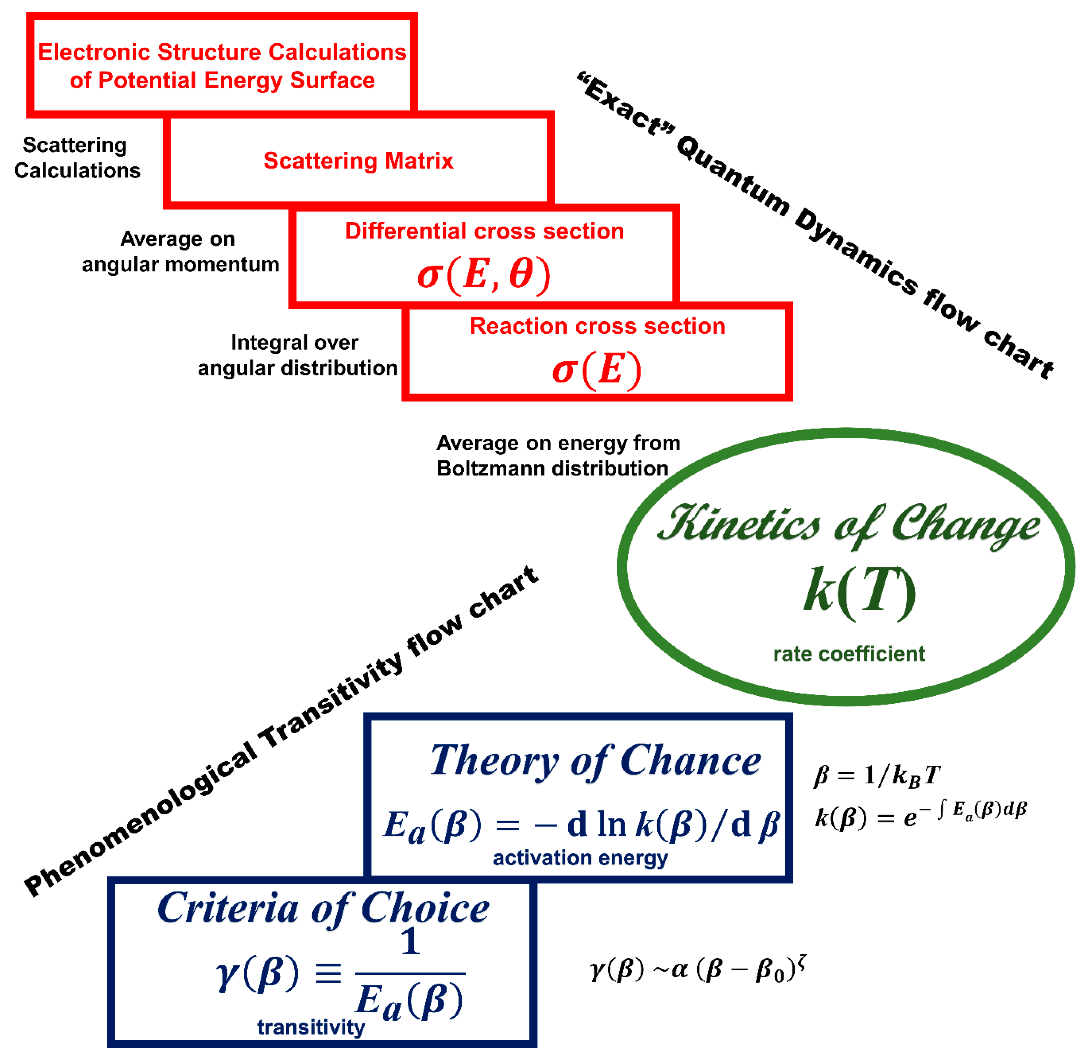
:1. Introduction
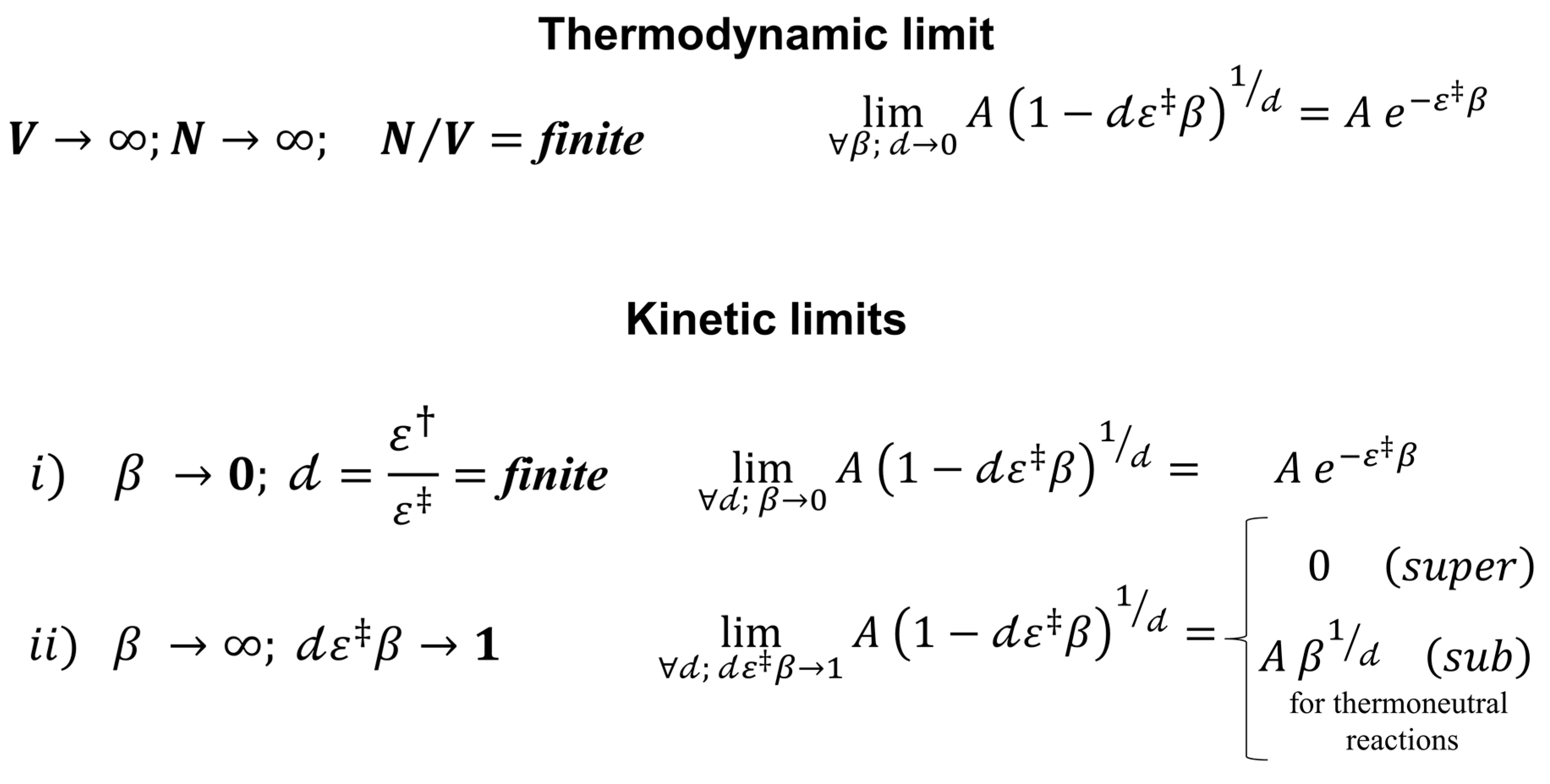
2. Thermodynamic versus Kinetic Limits, Revisited
2.1. The Exponential as Limit of Euler’s Succession: Role in the Early Kinetic Theory of Gases
2.2. The Thermodynamic Limit: The Contribution of Fowler and Collaborators
2.3. Avoiding the Thermodynamic Limit Describes Nonlinearities of Arrhenius Plots
2.4. Architecting the Transitivity Concept
2.4.1. Tolman’s Theorem and the Apparent Activation Energy
2.4.2. Planck Black-Body Radiation and Reciprocal Energy
2.4.3. Activation and Transitivity: A Prototypical Unimolecular Reaction Model
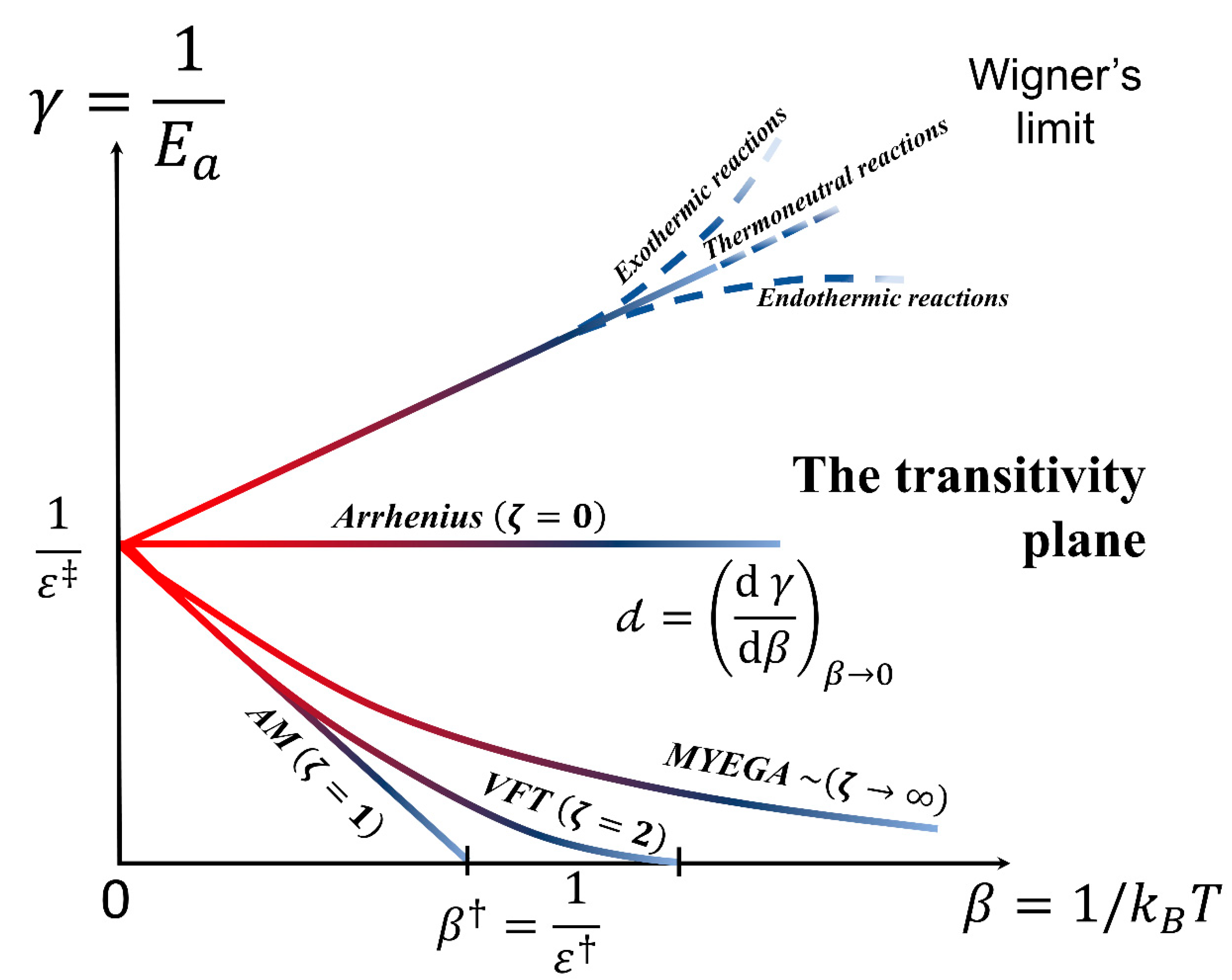
3. Scaling in the Transitivity Plane
3.1. Transitivity and Renormalization Group Coupling
3.2. Classes of Universal Behaviors
4. Perspectives on Rate Processes from the Arrhenius and the Transitivity Planes
- (i)
- The rates of biological processes are strongly affected at low temperatures by deviations from Arrhenius law; however there are large uncertainties especially when quantifying, as usual these deviations using the “Arrhenius Break Temperature” assumption, see previous discussions [3,60]. The difficulty of identifying a transition temperature in the Arrhenius plot for the respiration processes [60,102,103] can be easily overcome using the transitivity plot, emphasizing sudden transitions described within the Aquilanti–Mundim law (universality class with ζ = 1).
- (ii)
- Further applications concern the glass transition phenomenon occurring in a variety of materials: This is considered one of the most complex open problems in condensed matter physics. In the neighborhood of the glass transition temperature, the kinetic coefficients—diffusion, viscosity, and relaxation time—present deviations from the Arrhenius law specifically depending on the material composition. In reference [4], we examined the nonlinear temperature dependence of the relaxation time of propylene carbonate [98,99] from the transitivity plot: it is presented a perspective tool to observe a transition temperature connecting regimes described by two Aquilanti–Mundim straight lines in transitivity plane, and identifying the crossover temperature [93,94].
- (iii)
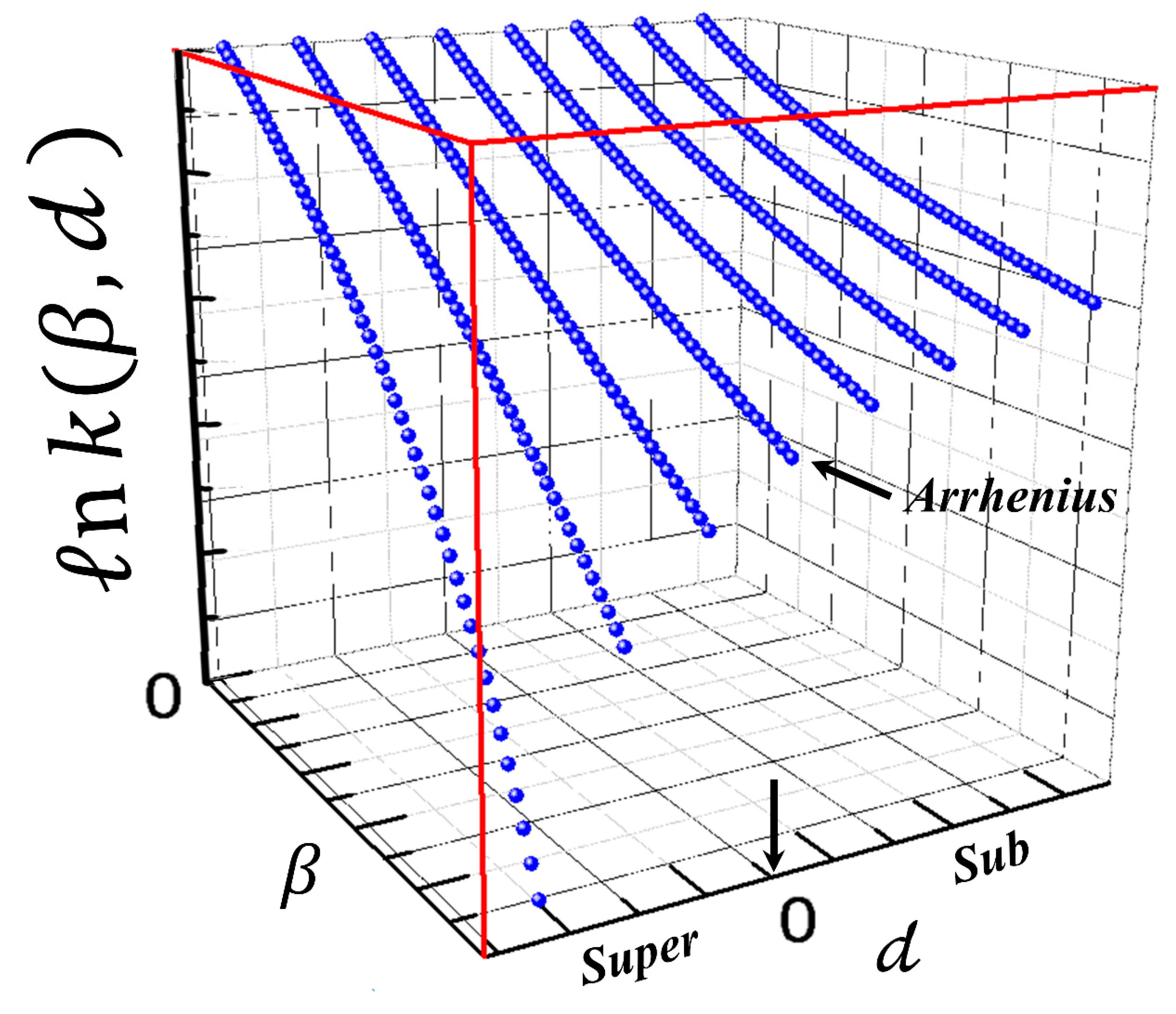
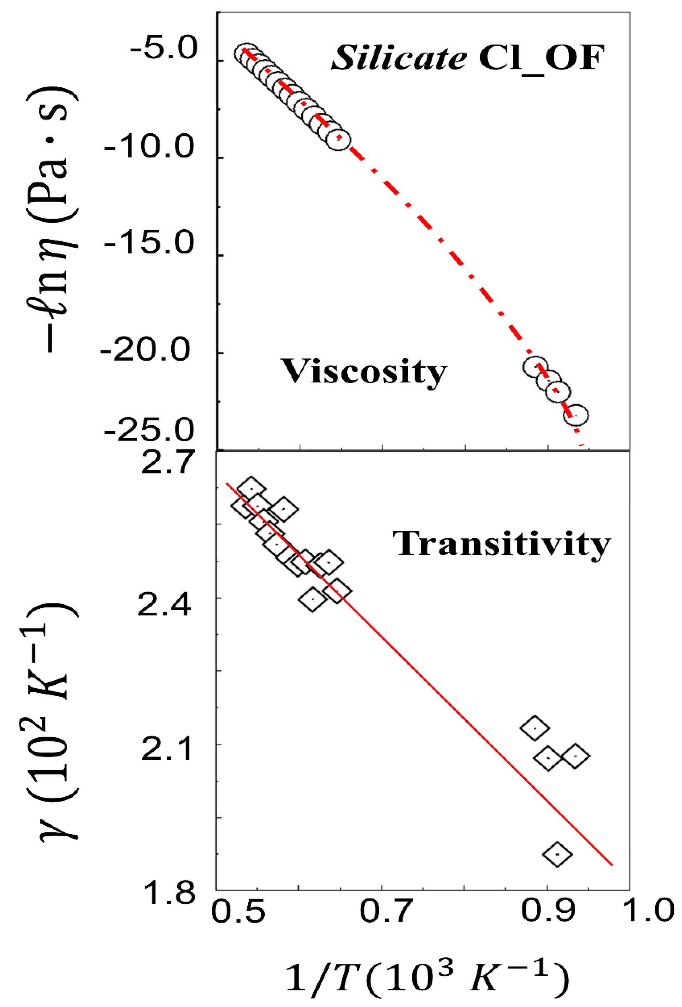
- Among phenomena akin to glass transitions but on extremely larger timescales, very important are those occurring in geochemical environments, where nonlinearity of the temperature dependence of the viscosity of rocks is often observed in the Arrhenius plots. In Figure 6, the nonlinearity in Arrhenius plot for Cl_OF silicate [49,104,105] also obeys the Aquilanti–Mundim law when analyzed in the transitivity plot: however, no transition temperature is revealed in this case.
5. Conclusions and Outlook
Author Contributions
Funding
Conflicts of Interest
Appendix A
Deformation of Statistical Distributions of Molecular Velocities and Kinetic Energies
References
- Aquilanti, V.; Coutinho, N.D.; Carvalho-Silva, V.H. Kinetics of Low-Temperature Transitions and Reaction Rate Theory from Non-Equilibrium Distributions. Philos. Trans. R. Soc. London A 2017, 375, 20160204. [Google Scholar] [CrossRef] [PubMed]
- Aquilanti, V.; Borges, E.P.; Coutinho, N.D.; Mundim, K.C.; Carvalho-Silva, V.H. From statistical thermodynamics to molecular kinetics: the change, the chance and the choice. Rend. Fis. Acc. Lincei. 2018, 28, 787–802. [Google Scholar] [CrossRef]
- Carvalho-Silva, V.H.; Coutinho, N.D.; Aquilanti, V. Temperature dependence of rate processes beyond Arrhenius and Eyring: Activation and Transitivity. Front. Chem. 2019, 7, 380. [Google Scholar] [CrossRef] [Green Version]
- Machado, H.G.; Sanches-Neto, F.O.; Coutinho, N.D.; Mundim, K.C.; Palazzetti, F.; Carvalho-Silva, V.H. “Transitivity”: a code for computing kinetic and related parameters in chemical transformations and transport phenomena. Molecules 2019, 24, 3478. [Google Scholar] [CrossRef] [Green Version]
- Arrhenius, S. On the reaction rate of the inversion of non-refined sugar upon souring. Z. Phys. Chem. 1889, 4, 226–248. [Google Scholar]
- van’t Hoff, J.H. Études de Dynamique Chimique; Frederik Muller: Amsterdam, The Netherlands, 1884. [Google Scholar]
- Laidler, K.J. The development of the Arrhenius equation. J. Chem. Educ. 1984, 61, 494. [Google Scholar] [CrossRef]
- Darwin, C.G.; Fowler, R.H. XLIV. On the partition of energy. Philos. Mag. J. Sci. 1922, 44, 450–479. [Google Scholar] [CrossRef]
- Darwin, C.G.; Fowler, R.H. LXXI. On the partition of energy—Part II. Statistical principles and thermodynamics. Philos. Mag. J. Sci. 1922, 44, 823–842. [Google Scholar] [CrossRef]
- Fowler, R.H. Statistical Mechanics: The Theory of the Properties of Matter in Equilibrium; The University Press: Cambridge, UK, 1929. [Google Scholar]
- Brush, S.G.; Hall, N.S. The Kinetic Theory of Gases: An Anthology of Classic Papers with Historical Commentary. In History of Modern Physical Sciences; Imperial College Press: London, UK, 2003; Volume 1. [Google Scholar]
- Gibbs, J.W. Elementary Principles in Statistical Mechanics: Developed with Especial Reference to the Rational Foundation of Thermodynamics; C. Scribner’s Sons: New York, NY, USA, 1902. [Google Scholar]
- Glasstone, S.; Laidler, K.J.; Eyring, H. The Theory of Rate Processes: The Kinetics of Chemical Reactions, Viscosity, Diffusion and Electrochemical Phenomena. In International Chemical Series; McGraw-Hill: New York, NY, USA, 1941. [Google Scholar]
- Eyring, H.; Walter, J. An elementary formulation of statistical mechanics. J. Chem. Educ. 1941, 18, 73. [Google Scholar] [CrossRef]
- Walter, J.E.; Eyring, H.; Kimball, G.E. Quantum Chemistry; Wiley & Sons: New York, NY, USA, 1944. [Google Scholar]
- Johnson, F.H.; Eyring, H.; Polissar, M.J. The Kinetic Basis of Molecular Biology; Wiley & Sons: New York, NY, USA, 1954. [Google Scholar]
- Maxwell, J.C. XX. Illustrations of the dynamical theory of gases. Philos. Mag. 1860, 19, 377–391. [Google Scholar] [CrossRef]
- Maxwell, J.C. On the Dynamical Theory of Gases. Philos. Trans. 1866, 157, 49–88. [Google Scholar]
- Aquilanti, V.; Cavalli, S.; Fazio, D. De; Volpi, A.; Aguilar, A.; Lucas, J.M. Benchmark rate constants by the hyperquantization algorithm. The F + H2 reaction for various potential energy surfaces: features of the entrance channel and of the transition state, and low temperatur e reactivity. Chem. Phys. 2005, 308, 237–253. [Google Scholar] [CrossRef]
- De Fazio, D.; Aquilanti, V.; Cavalli, S. Quantum Dynamics and Kinetics of the F + H2 and F + D2 Reactions at Low and Ultra-Low Temperatures. Front. Chem. 2019, 7, 328. [Google Scholar] [CrossRef] [Green Version]
- De Fazio, D. The H + HeH+→ He + H2+ reaction from the ultra-cold regime to the three-body breakup: Exact quantum mechanical integral cross sections and rate constants. Phys. Chem. Chem. Phys. 2014, 16, 11662–11672. [Google Scholar] [CrossRef]
- Cavalli, S.; De Fazio, D.; Aquilanti, V. Quantum effects in the F+H2 and F+D2. Front. Chem. 2019, 7, 328. [Google Scholar]
- Ruggeri, T.; Sugiyama, M. Rational extended thermodynamics: a link between kinetic theory and continuum theory. Rend. Fis. Acc. Lincei 2020, 31, 33–38. [Google Scholar] [CrossRef]
- Cercignani, C. Ludwig Boltzmann: The Man Who Trusted Atoms; Oxford University Press: Oxford, UK, 2006. [Google Scholar]
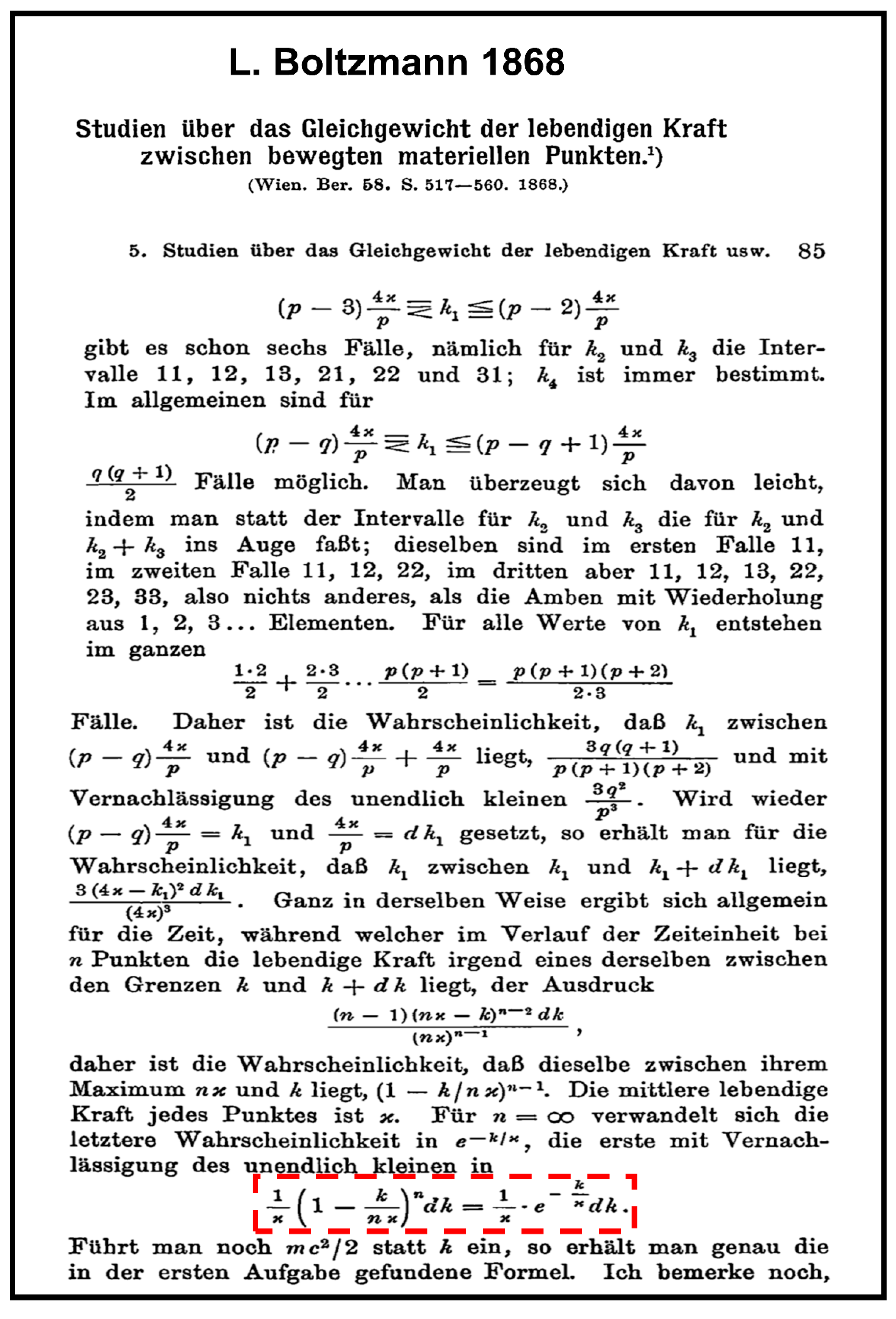
- Boltzmann, L. Studien über das Gleichgewicht der lebendigen Kraft zwischen bewegten materiellen Punkten. Wien. Ber. 1868, 58, 517–560. [Google Scholar]
- Costantini, D.; Garibaldi, U. A Probabilistic Foundation of Elementary Particle Statistics. Part I. Stud. Hist. Philos. Sci. B Stud. Hist. Philos. Mod. Phys. 1998, 28, 483–506. [Google Scholar] [CrossRef]
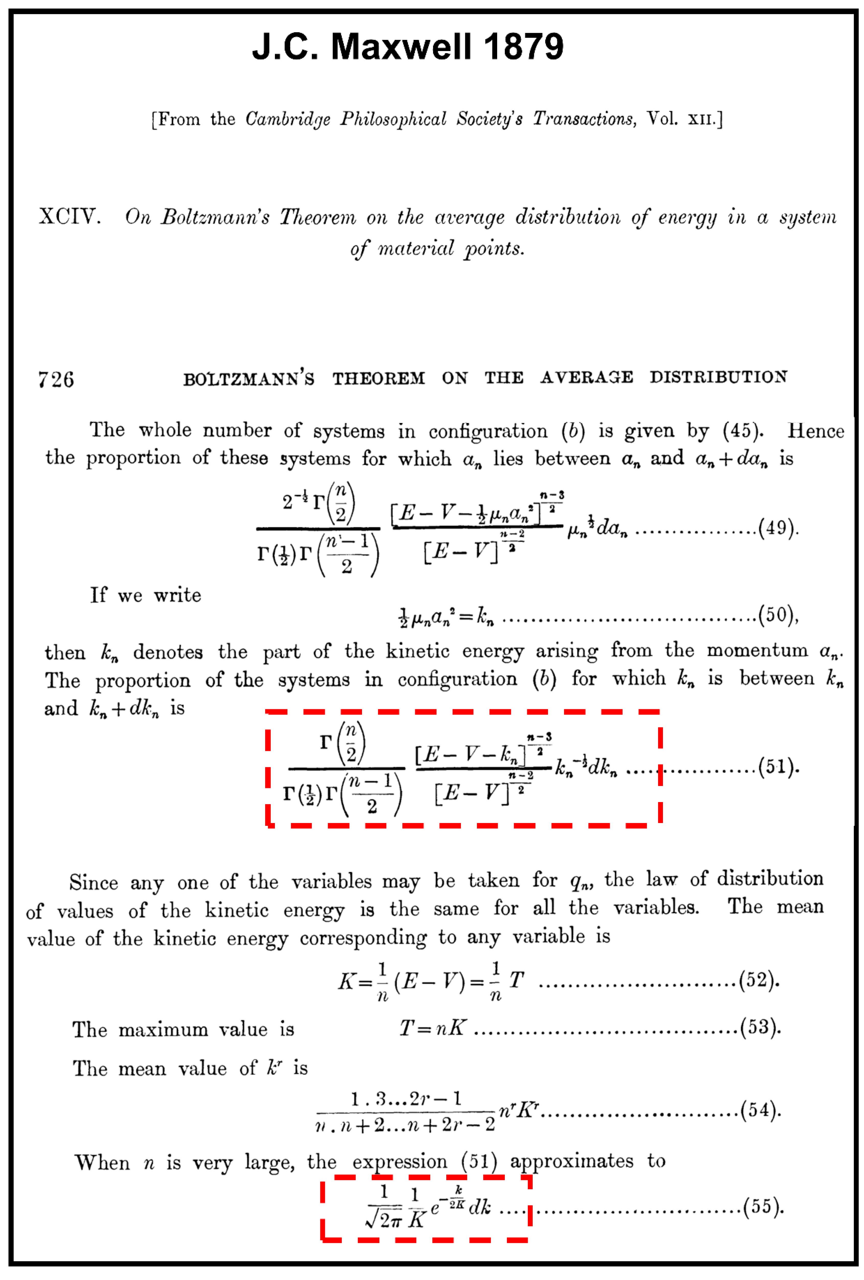
- Maxwell, J.C. On Boltzmann’s theorem on the average distribution of energy in a system of material points. Trans. Cambridge Phil. Soc. 1879, 12, 713–741. [Google Scholar]
- Jeans, J. The Dynamical Theory of Gases; Cambridge University Press: Cambridge, UK, 1916. [Google Scholar]
- Uhlenbeck, G.E.; Goudsmit, S. Statistical energy distributions for a small number of particles. Zeeman Verhandenlingen 1935, Martinus N, 201–211. [Google Scholar]
- Adib, A.B.; Moreira, A.A.; Andrade Jr, J.S.; Almeida, M.P. Tsallis thermostatistics for finite systems: a Hamiltonian approach. Phys. A Stat. Mech. its Appl. 2003, 322, 276–284. [Google Scholar] [CrossRef] [Green Version]
- Kennard, E.H. Kinetic Theory of Gases: With an Introduction to Statistical Mechanics. In International Series in Pure and Applied Physics; McGraw-Hill: New York, NY, USA, 1938. [Google Scholar]
- Tolman, R.C. Statistical Mechanics with Applications to Physics and Chemistry. Chem. Eng. News 1927, 5, 16. [Google Scholar]
- Tolman, R.C. The Principles of Statistical Mechanics; Oxford University: London, UK, 1938. [Google Scholar]
- Condon, E.U. A Simple Derivation of the Maxwell-Boltzmann Law. Phys. Rev. 1938, 54, 937–940. [Google Scholar] [CrossRef]
- Fowler, R.H.; Guggenheim, E.A. Statistical Thermodynamics: A Version of Statistical Mechanics for Students of Physics and Chemistry; Macmillan: London, UK, 1939. [Google Scholar]
- Fowler, R.; Guggenheim, E.A. Statistical Thermodynamics; Cambridge University Press: Cambridge, UK, 1939. [Google Scholar]
- Schrodinger, E. Statistical Thermodynamics: A Course of Seminar Lectures; Cambridge University Press: London, UK, 1948. [Google Scholar]
- Yang, C.N.; Lee, T.D. Statistical theory of equations of state and phase transitions. I. Theory of condensation. Phys. Rev. 1952. [Google Scholar] [CrossRef]
- Lee, T.D.; Yang, C.N. Statistical theory of equations of state and phase transitions. II. Lattice gas and ising model. Phys. Rev. 1952. [Google Scholar] [CrossRef]
- Huang, K. Statistical Mechanics, 2nd ed.; John Wiley and Sons: New York, NY, USA, 1987. [Google Scholar]
- Van Vliet, C.M. Equilibrium and Non-Equilibrium Statistical Mechanics; World Scientific: Singapore, 2008. [Google Scholar]
- Pathria, R.K.; Beale, P.D. Statistical Mechanics, 3rd ed.; Academic Press: Cambridge, MA, USA, 2007. [Google Scholar]
- Blundell, S.J.; Blundell, K.M. Concepts in Thermal Physics; Oxford University Press: Oxford, UK, 2010. [Google Scholar]
- Kuzemsky, A.L. Thermodynamic Limit in Statistical Physics. Int. J. Mod. Phys. B 2014, 28, 1430004. [Google Scholar] [CrossRef]
- Hill, T.L. Statistical Mechanics: Principles and Selected Applications; McGraw-Hill: New York, NY, USA, 1956. [Google Scholar]
- Landau, L.D.; Lifshitz, E.M. Statistical Physics, 5th ed.; Pergamon Press: Oxford, UK, 1958. [Google Scholar]
- Lavenda, B.H. Statistical Physics: A Probabilistic Approach; Dover Publications: Mineola, NY, USA, 2016. [Google Scholar]
- Hinshelwood, C.N. The kinetics of chemical change. J. Chem. Educ. 1940, 39, 79. [Google Scholar]
- Giordano, D.; Russell, J.K.; Dingwell, D.B. Viscosity of magmatic liquids: A model. Earth Planet. Sci. Lett. 2008, 271, 123–124. [Google Scholar] [CrossRef]
- Angell, C.A. Formation of glasses from liquids and biopolymers. Science 1995, 267, 1924–1935. [Google Scholar] [CrossRef] [Green Version]
- Kohen, A.; Cannio, R.; Bartolucci, S.; Klinman, J.P. Enzyme dynamics and hydrogen tunnelling in a thermophilic alcohol dehydrogenase. Nature 1999, 399, 496–499. [Google Scholar] [CrossRef]
- Limbach, H.-H.; Miguel Lopez, J.; Kohen, A. Arrhenius curves of hydrogen transfers: tunnel effects, isotope effects and effects of pre-equilibria. Philos. Trans. R. Soc. Lond. B. Biol. Sci. 2006, 361, 1399–1415. [Google Scholar] [CrossRef] [PubMed] [Green Version]
- Smith, I.W.M. The temperature-dependence of elementary reaction rates: beyond Arrhenius. Chem. Soc. Rev. 2008, 37, 812–826. [Google Scholar] [CrossRef]
- Capitelli, M.; Pietanza, L.D. Past and present aspects of Italian plasma chemistry. Rend. Fis. Acc. Lincei 2019, 30, 31–48. [Google Scholar] [CrossRef]
- Kubo, K. A view on the break in the Arrhenius plots. J. Theor. Biol. 1985, 115, 551–569. [Google Scholar] [CrossRef]
- Nishiyama, M.; Kleijn, S.; Aquilanti, V.; Kasai, T. Temperature dependence of respiration rates of leaves, 18O-experiments and super-Arrhenius kinetics. Chem. Phys. Lett. 2009, 482, 325–329. [Google Scholar] [CrossRef]
- Müller, I. The coldness, a universal function in thermoelastic bodies. Arch. Ration. Mech. Anal. 1971, 41, 319–332. [Google Scholar] [CrossRef]
- Vieira, C.L.; Sanches Neto, F.O.; Carvalho-Silva, V.H.; Signini, R. Design of apolar chitosan-type adsorbent for removal of Cu(II) and Pb(II): An experimental and DFT viewpoint of the complexation process. J. Environ. Chem. Eng. 2019, 7, 103070. [Google Scholar] [CrossRef]
- Silva, V.H.C.; Aquilanti, V.; De Oliveira, H.C.B.; Mundim, K.C. Uniform description of non-Arrhenius temperature dependence of reaction rates, and a heuristic criterion for quantum tunneling vs classical non-extensive distribution. Chem. Phys. Lett. 2013, 590, 201–207. [Google Scholar] [CrossRef] [Green Version]
- Aquilanti, V.; Mundim, K.C.; Elango, M.; Kleijn, S.; Kasai, T. Temperature dependence of chemical and biophysical rate processes: Phenomenological approach to deviations from Arrhenius law. Chem. Phys. Lett. 2010, 498, 209–213. [Google Scholar] [CrossRef]
- Gell-Mann, M.; Tsallis, C. Nonextensive Entropy: Interdisciplinary Applications; Oxford University Press: New York, NY, USA, 2004. [Google Scholar]
- Tsallis, C. Possible generalization of Boltzman-Gibbs Statistics. J. Stat. Phys. 1988, 52, 479–487. [Google Scholar] [CrossRef]
- Carvalho-Silva, V.H.; Aquilanti, V.; de Oliveira, H.C.B.; Mundim, K.C. Deformed transition-state theory: Deviation from Arrhenius behavior and application to bimolecular hydrogen transfer reaction rates in the tunneling regime. J. Comput. Chem. 2017, 38, 178–188. [Google Scholar] [CrossRef] [PubMed]
- Sanches-Neto, F.O.; Coutinho, N.D.; Silva, V. A novel assessment of the role of the methyl radical and water formation channel in the CH3OH + H reaction. Phys. Chem. Chem. Phys. 2017, 19, 24467–24477. [Google Scholar] [CrossRef] [PubMed]
- Aquilanti, V.; Mundim, K.C.; Cavalli, S.; De Fazio, D.; Aguilar, A.; Lucas, J.M. Exact activation energies and phenomenological description of quantum tunneling for model potential energy surfaces. the F + H2 reaction at low temperature. Chem. Phys. 2012, 398, 186–191. [Google Scholar] [CrossRef]
- Coutinho, N.D.; Silva, V.H.C.; de Oliveira, H.C.B.; Camargo, A.J.; Mundim, K.C.; Aquilanti, V. Stereodynamical Origin of Anti-Arrhenius Kinetics: Negative Activation Energy and Roaming for a Four-Atom Reaction. J. Phys. Chem. Lett. 2015, 6, 1553–1558. [Google Scholar] [CrossRef]
- Coutinho, N.D.; Sanches-Neto, F.O.; Carvalho-Silva, V.H.; de Oliveira, H.C.B.; Ribeiro, L.A.; Aquilanti, V. Kinetics of the OH + HCl ⟶H2O+Cl reaction: rate determining roles of stereodynamics and roaming, and of quantum tunnelling. J. Comput. Chem. 2018, 39, 2508–2516. [Google Scholar] [CrossRef]
- Coutinho, N.D.; Aquilanti, V.; Sanches-Neto, F.O.; Vaz, E.C.; Carvalho-Silva, V.H. First-principles molecular dynamics and computed rate constants for the series of OH-HX reactions (X= H or the halogens): non-Arrhenius kinetics, stereodynamics and quantum tunnel. In Proceedings of the 18th International Conference on Computational Science and Applications, ICCSA 2018, Melbourne, VIC, Australia, 2–5 July 2018. [Google Scholar]
- Biró, T.; Ván, P.; Barnaföldi, G.; Ürmössy, K. Statistical Power Law due to Reservoir Fluctuations and the Universal Thermostat Independence Principle. Entropy 2014, 16, 6497–6514. [Google Scholar] [CrossRef]
- Bíró, G.; Barnaföldi, G.; Biró, T.; Ürmössy, K.; Takács, Á.; Bíró, G.; Barnaföldi, G.G.; Biró, T.S.; Ürmössy, K.; Takács, Á. Systematic Analysis of the Non-Extensive Statistical Approach in High Energy Particle Collisions—Experiment vs. Theory. Entropy 2017, 19, 88. [Google Scholar] [CrossRef]
- Junior, A.C.D.P.R.; Cruz, C.; Santana, W.S.; Moret, M.A. Characterization of the non-Arrhenius behavior of supercooled liquids by modeling non-additive stochastic systems. Phys. Rev. E 2019, 100, 22139. [Google Scholar]
- Junior, A.C.D.P.R.; Cruz, C.; Santana, W.S.; Junior, E.B.A.; Moret, M.A. Non-Arrhenius behavior and fragile-to-strong transition of glass-forming liquids. Phys. Rev. E 2020, 101, 042131. [Google Scholar]
- Bradley, R.E.; Sandifer, C.E. Cauchy’s Cours d’Analyse: An Annotated Translation; Springer: Pasadena, CA, USA, 2009. [Google Scholar]
- Wigner, E.P. On the Behavior of Cross Sections Near Thresholds. Phys. Rev. 1948, 73, 1002–1009. [Google Scholar] [CrossRef]
- Takayanagi, T. Theory of Atom Tunneling Reactions in the Gas Phase; Springer: Berlin, Germany, 2004; pp. 15–31. [Google Scholar]
- Sanches-Neto, F.O.; Coutinho, N.D.; Palazzetti, F.; Carvalho-Silva, V.H. Temperature dependence of rate constants for the H(D) + CH4 reaction in gas and aqueous phase: deformed Transition-State Theory study including quantum tunneling and diffusion effects. Struct. Chem. 2019, 31, 609–617. [Google Scholar] [CrossRef]
- Abe, S.; Okamoto, Y. Nonextensive Statistical Mechanics and Its Applications. In Lecture Notes in Physics; Springer: Berlin, Germany, 2008. [Google Scholar]
- Tsallis, C. Introduction to Nonextensive Statistical Mechanics: Approaching a Complex World; Springer: New York, NY, USA, 2009. [Google Scholar]
- Tolman, R.C. Statistical Merchanics Applied To Chemical Kinetics. J. Am. Chem. Soc. 1920, 42, 2506–2528. [Google Scholar] [CrossRef]
- Vogel, H. Das temperature-abhangigketsgesetz der viskositat von flussigkeiten. Phys. Z 1921, 22, 645–646. [Google Scholar]
- Fulcher, G.S. Analysis of Recent Measurements of the Viscosity of Glasses. J. Am. Ceram. Soc. 1925, 8, 339–355. [Google Scholar] [CrossRef]
- Tammann, G.; Hesse, W. Die Abhängigkeit der Viscosität von der Temperatur bie unterkühlten Flüssigkeiten. Zeitschrift für Anorg. und Allg. Chemie 1926, 156, 245–257. [Google Scholar] [CrossRef]
- Laidler, K.J. A Glossary of Terms Used in Chemical Kinetics, Including Reaction Dynamics. Pure Appl. Chem. 1996, 68, 149–192. [Google Scholar] [CrossRef] [Green Version]
- Planck, M.; Press, P. On the Theory of the Energy Distribution Law of the Normal Spectrum. Verh. Deutsch. Phys. Ges. 1900, 237, 1–8. [Google Scholar]
- Slater, N.B. Theory of Unimolecular Reactions; Cornell University Press: Ithaca, NY, USA, 1959. [Google Scholar]
- Marcelin, R. Contribution à l’étude de la cinétique physico-chimique. Ann. Phys. (Paris). 1915, 9, 120–231. [Google Scholar] [CrossRef] [Green Version]
- Callan, C.G. Broken scale invariance in scalar field theory. Phys. Rev. D 1970, 2, 1541. [Google Scholar] [CrossRef]
- Symanzik, K. Small-distance-behaviour analysis and Wilson expansions. Commun. Math. Phys. 1971, 23, 49–86. [Google Scholar] [CrossRef]
- Wilson, K.G. Renormalization group and critical phenomena. I. Renormalization group and the Kadanoff scaling picture. Phys. Rev. B 1971, 4, 3174. [Google Scholar] [CrossRef] [Green Version]
- Weinberg, S. The Quantum Theory of Fields; Cambridge University Press: Cambridge, UK, 1995; Volume 2. [Google Scholar]
- Gupta, S. Effective Field Theories. In Lecture 2: Wilsonian Renormalization. In Proceedings of the Mini School 2016, IACS Kolkata, India, 29 February–4 March 2016. [Google Scholar]
- Honig, J.M.; Spalek, J. A Primer to the Theory of Critical Phenomena; Elsevier Science: Amsterdam, The Netherlands, 2018. [Google Scholar]
- Mallamace, F.; Branca, C.; Corsaro, C.; Leone, N.; Spooren, J.; Chen, S.H.; Stanley, H.E. Transport properties of glass-forming liquids suggest that dynamic crossover temperature is as important as the glass transition temperature. Proc. Natl. Acad. Sci. USA 2010, 107, 22457–22462. [Google Scholar] [CrossRef] [PubMed] [Green Version]
- Martinez-Garcia, J.C.; Martinez-Garcia, J.; Rzoska, S.J.; Hulliger, J. The new insight into dynamic crossover in glass forming liquids from the apparent enthalpy analysis. J. Chem. Phys. 2012, 137, 064501. [Google Scholar] [CrossRef] [PubMed] [Green Version]
- Souletie, J. The glass transition: dynamic and static scaling approach. J. Phys. 1990, 51, 883–898. [Google Scholar] [CrossRef]
- Mauro, J.C.; Yue, Y.; Ellison, A.J.; Gupta, P.K.; Allan, D.C. Viscosity of glass-forming liquids. Proc. Natl. Acad. Sci. USA 2009, 106, 19780–19784. [Google Scholar] [CrossRef] [Green Version]
- Souletie, J.; Tholence, J.L. Critical slowing down in spin glasses and other glasses: Fulcher versus power law. Phys. Rev. B 1985, 32, 516. [Google Scholar] [CrossRef]
- Stickel, F.; Fischer, E.W.; Richert, R. Dynamics of glass-forming liquids. II. Detailed comparison of dielectric relaxation, de-conductivity, and viscosity data. J. Chem. Phys. 1996, 104, 2043. [Google Scholar] [CrossRef]
- Drozd-Rzoska, A. Universal behavior of the apparent fragility in ultraslow glass forming systems. Sci. Rep. 2019, 9, 6816. [Google Scholar] [CrossRef]
- Coutinho, N.D.; Silva, V.H.C.; Mundim, K.C.; de Oliveira, H.C.B. Description of the effect of temperature on food systems using the deformed Arrhenius rate law: deviations from linearity in logarithmic plots vs. inverse temperature. Rend. Fis. Acc. Lincei 2015, 26, 141–149. [Google Scholar] [CrossRef]
- Cavalli, S.; Aquilanti, V.; Mundim, K.C.; De Fazio, D. Theoretical reaction kinetics astride the transition between moderate and deep tunneling regimes: The F + HD case. J. Phys. Chem. A 2014, 118, 6632–6641. [Google Scholar] [CrossRef]
- Crozier, W.J.; Stier, T.B. Critical Thermal Increments for Rhythmic Respiratory Movements of Insects. J. Gen. Physiol. 1925, 7, 429–447. [Google Scholar] [CrossRef] [PubMed] [Green Version]
- Cossins, A.R.; Bowler, K. Temperature Biology of Animals; Chapman and Hall: London, UK, 1987. [Google Scholar]
- Giordano, D.; Dingwell, D.B. Non-Arrhenian multicomponent melt viscosity: A model. Earth Planet. Sci. Lett. 2003, 208, 337–349. [Google Scholar] [CrossRef]
- Giordano, D.; Mangiacapra, A.; Potuzak, M.; Russell, J.K.; Romano, C.; Dingwell, D.B.; Di Muro, A. An expanded non-Arrhenian model for silicate melt viscosity: A treatment for metaluminous, peraluminous and peralkaline liquids. Chem. Geol. 2006, 229, 42–56. [Google Scholar] [CrossRef]
- Suleimanov, Y. V.; Collepardo-Guevara, R.; Manolopoulos, D.E. Bimolecular reaction rates from ring polymer molecular dynamics: Application to H + CH4→ H2 + CH3. J. Chem. Phys. 2011, 134, 044131. [Google Scholar] [CrossRef] [Green Version]
- Zhang, Y.; Stecher, T.; Cvitaš, M.T.; Althorpe, S.C. Which Is Better at Predicting Quantum-Tunneling Rates: Quantum Transition-State Theory or Free-Energy Instanton Theory? J. Phys. Chem. Lett. 2014, 5, 3976–3980. [Google Scholar] [CrossRef]
- Richardson, J.O. Ring-Polymer Approaches to Instanton Theory; University of Cambridge: London, UK, 2012. [Google Scholar]
- Janssen, L.M.C. Mode-coupling theory of the glass transition: A primer. Front. Phys. 2018, 6, 97. [Google Scholar] [CrossRef] [Green Version]
- Müller, I.; Ruggeri, T. Rational Extended Thermodynamics; Springer: New York, NY, USA, 1998. [Google Scholar]
- Williams, M.L.; Landel, R.F.; Ferry, J.D. Temperature Dependence of Relaxation Mechanisms in Amorphous Polymers and Other Glass-Forming Liquids. Phys. Rev. 1955, 98, 1549. [Google Scholar] [CrossRef]
- Bělehrádek, J. A unified theory of cellular rate processes based upon an analysis of temperature action. Protoplasma 1957, 48, 53–71. [Google Scholar] [CrossRef]
- Bässler, H. Viscous flow in supercooled liquids analyzed in terms of transport theory for random media with energetic disorder. Phys. Rev. Lett. 1987, 58, 767–770. [Google Scholar] [CrossRef]
- Nakamura, K.; Takayanagi, T.; Sato, S. A modified arrhenius equation. Chem. Phys. Lett. 1989, 160, 295–298. [Google Scholar] [CrossRef]
- Gentili, P.L. The fuzziness of the molecular world and its perspectives. Molecules 2018, 23, 2074. [Google Scholar] [CrossRef] [PubMed] [Green Version]
- Zadeh, L.A. Toward human level machine intelligence - Is it achievable? the need for a paradigm shift. IEEE Comput. Intell. Mag. 2008, 3, 11–22. [Google Scholar] [CrossRef]
- Duffin, R.J.; Zener, C. Geometric programming and the Darwin-Fowler method in statistical mechanics. J. Phys. Chem. 1970, 74, 2419–2423. [Google Scholar] [CrossRef]
- Agrawal, A.; Diamond, S.; Boyd, S. Disciplined geometric programming. Optim. Lett. 2019, 13, 961–976. [Google Scholar] [CrossRef] [Green Version]
- Kamel, A.M.; Dorrah, H.T.; Farid, S.; Eid, S.; Mohammed, A. Fuzzy Geometric Programming Optimization using New Arithmetic Fuzzy Logic-based Representation. In Proceedings of the 14thInternational Middle East PowerSystems Conference (MEPCON’10), Cairo, Egypt, 19–21 December 2010. [Google Scholar]
- Mundim, K.C.; Tsallis, C. Geometry optimization and conformational analysis through generalized simulated annealing. Int. J. Quantum Chem. 1996, 58, 373–381. [Google Scholar] [CrossRef]
- Ilva, R. A Maxwellian Path to the q -Nonextensive Velocity Distribution Function. Phys. Lett. A 2008, 9601, 1–15. [Google Scholar]
- Silva, R.; Alcaniz, J.S. Negative heat capacity and non-extensive kinetic theory. Phys. Lett. Sect. A Gen. At. Solid State Phys. 2003, 313, 393–396. [Google Scholar] [CrossRef] [Green Version]
- Laidler, K. Chemical Kinetics. Harper Row 1987, 1, 233–270. [Google Scholar]


© 2020 by the authors. Licensee MDPI, Basel, Switzerland. This article is an open access article distributed under the terms and conditions of the Creative Commons Attribution (CC BY) license (http://creativecommons.org/licenses/by/4.0/).
Share and Cite
Carvalho-Silva, V.H.; Coutinho, N.D.; Aquilanti, V. From the Kinetic Theory of Gases to the Kinetics of Rate Processes: On the Verge of the Thermodynamic and Kinetic Limits. Molecules 2020, 25, 2098. https://doi.org/10.3390/molecules25092098
Carvalho-Silva VH, Coutinho ND, Aquilanti V. From the Kinetic Theory of Gases to the Kinetics of Rate Processes: On the Verge of the Thermodynamic and Kinetic Limits. Molecules. 2020; 25(9):2098. https://doi.org/10.3390/molecules25092098
Chicago/Turabian StyleCarvalho-Silva, Valter H., Nayara D. Coutinho, and Vincenzo Aquilanti. 2020. "From the Kinetic Theory of Gases to the Kinetics of Rate Processes: On the Verge of the Thermodynamic and Kinetic Limits" Molecules 25, no. 9: 2098. https://doi.org/10.3390/molecules25092098