
Detection and Quantification of Bisphenol A in Surface Water Using Absorbance–Transmittance and Fluorescence Excitation–Emission Matrices (A-TEEM) Coupled with Multiway Techniques

 ,
,
Abstract
:1. Introduction
2. Results
2.1. Absorbance, Excitation, and Emission Spectra
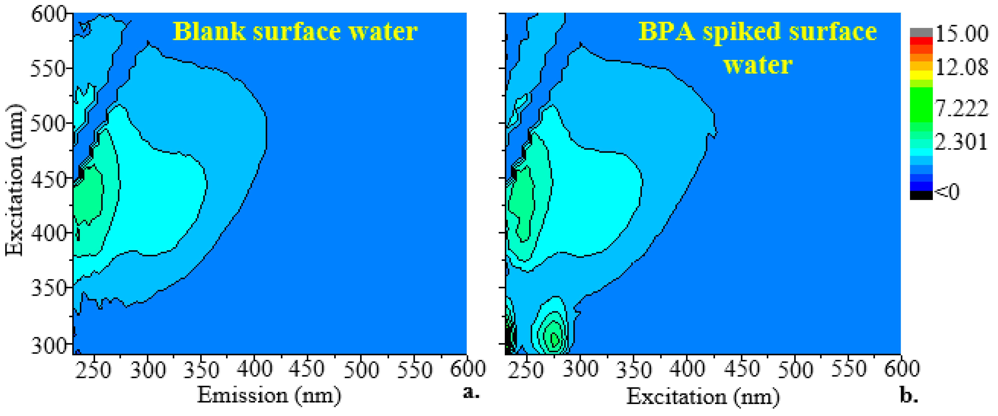
2.2. Excitation–Emission Matrix Signature for BPA
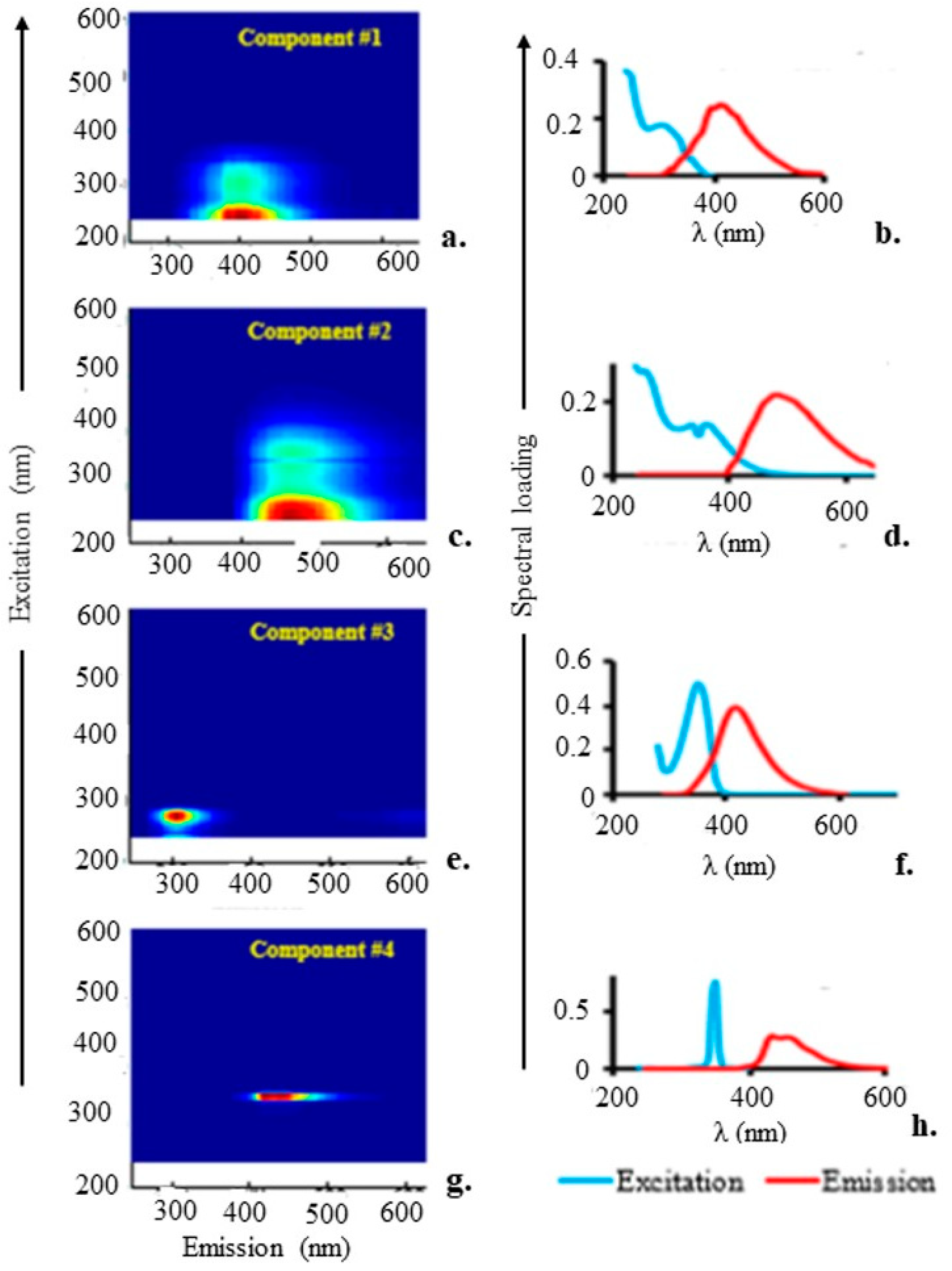
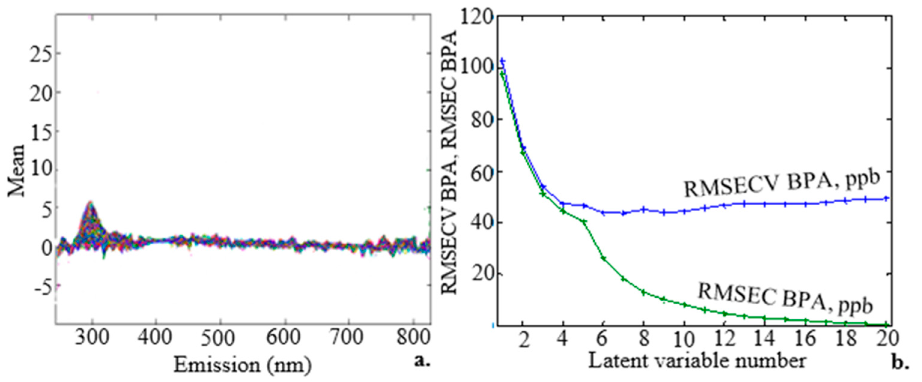
2.3. Construction and Validation of the PARAFAC Model
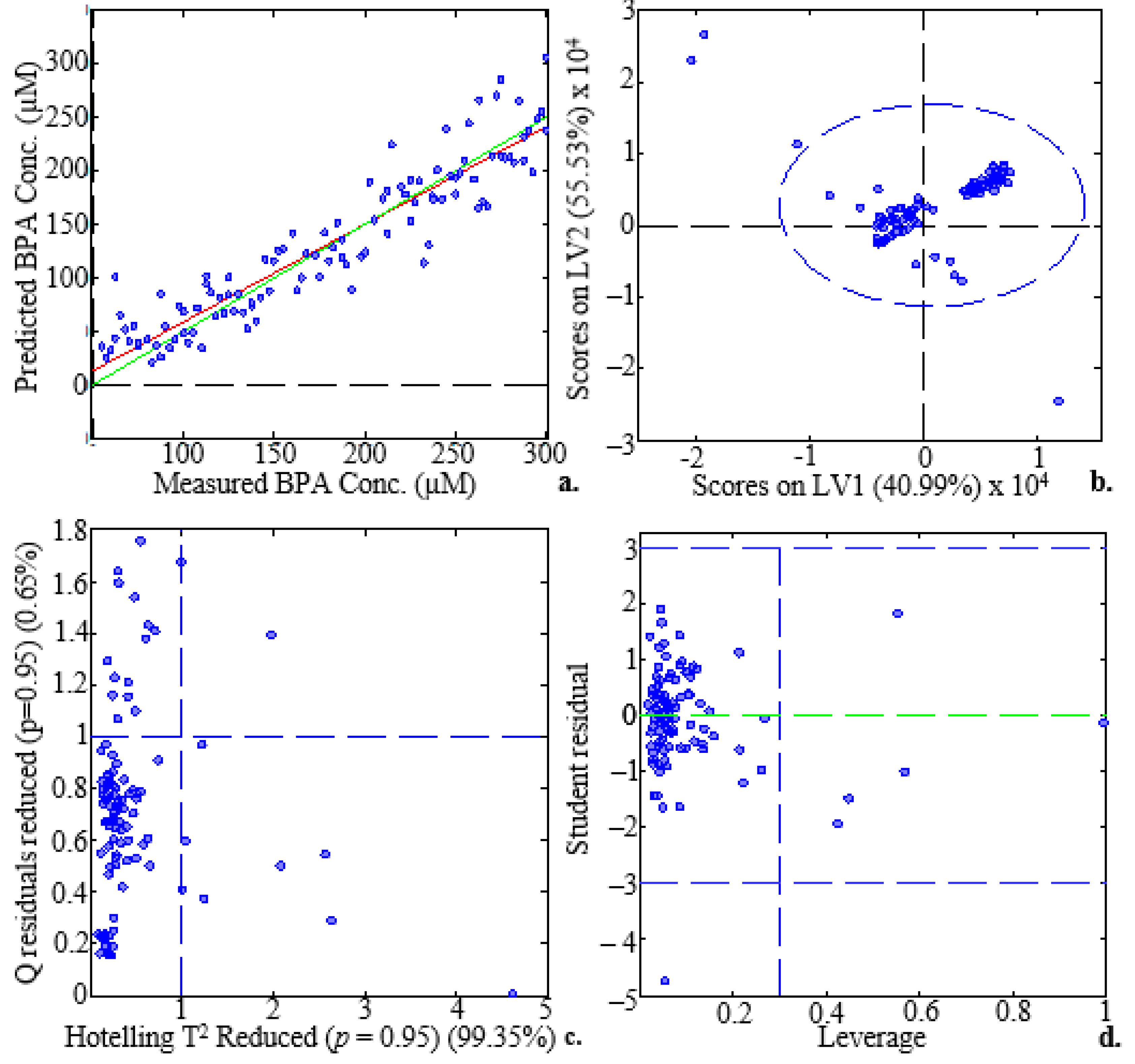
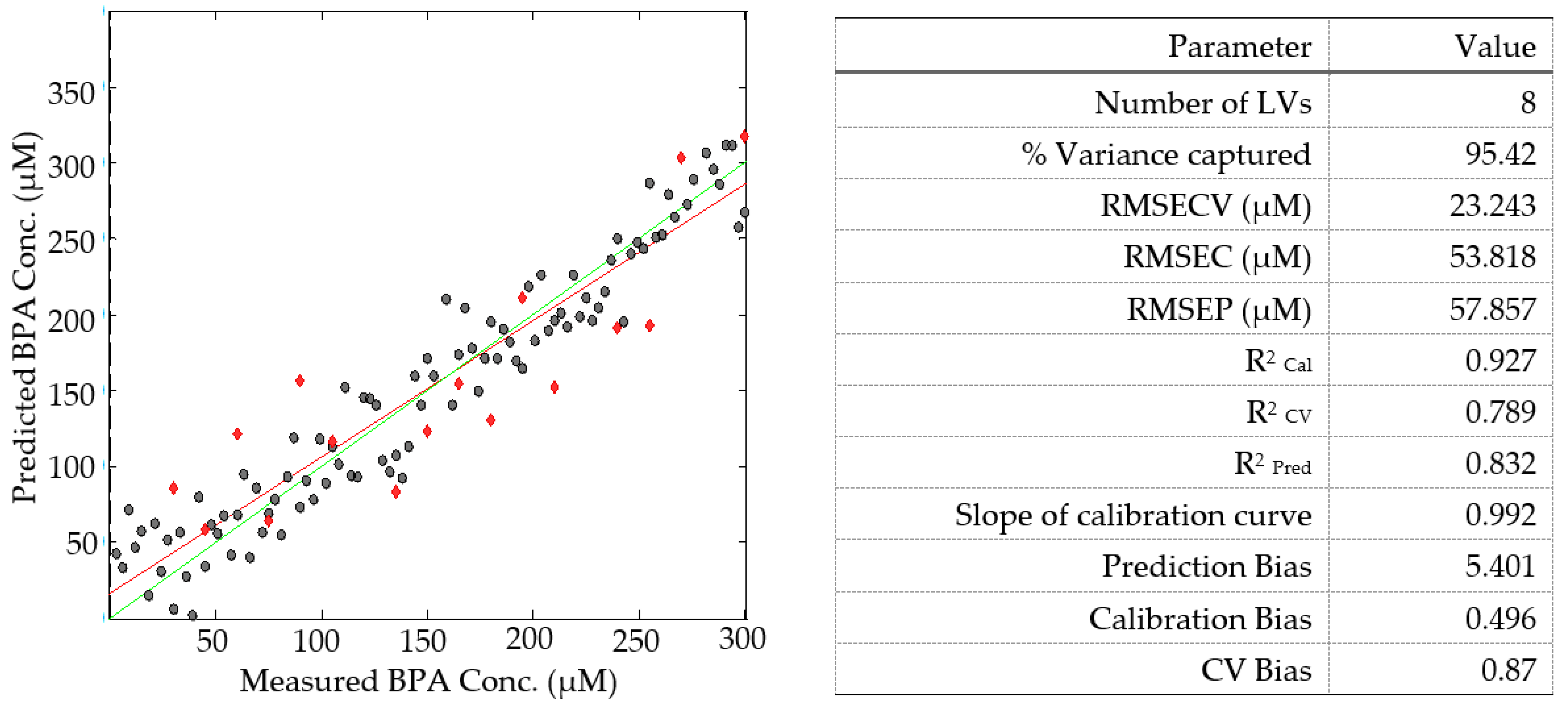
2.4. Construction of the PLS Model
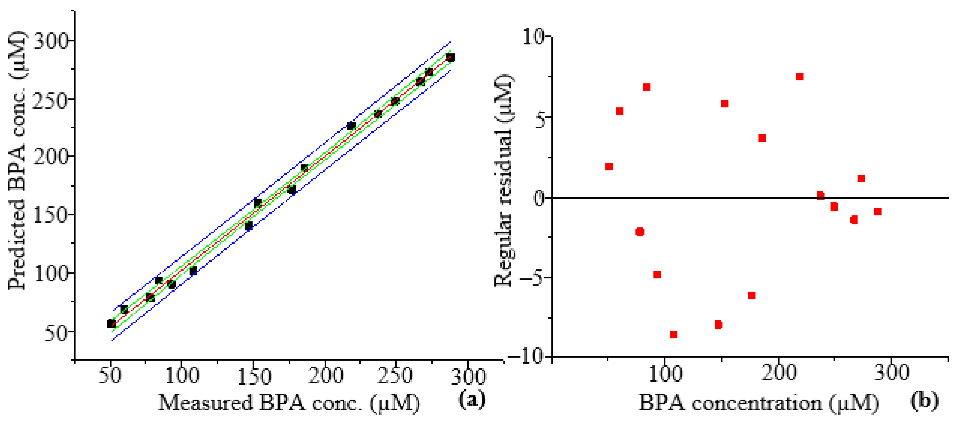
2.5. Validation of Spiked Samples
2.6. Method Sensitivity and Limits of Detection and Quantification
2.7. Recovery and Accuracy
3. Materials and Methods
3.1. Materials and Reagents
3.2. Sampling
3.3. Preparation of a Stock Solution and an Intermediate Standard Solution
3.4. Sample Preparation
3.5. Total Organic Carbon Determination
3.6. The Calibration of the A-TEEM Instrument
3.7. Instrumentation and Software
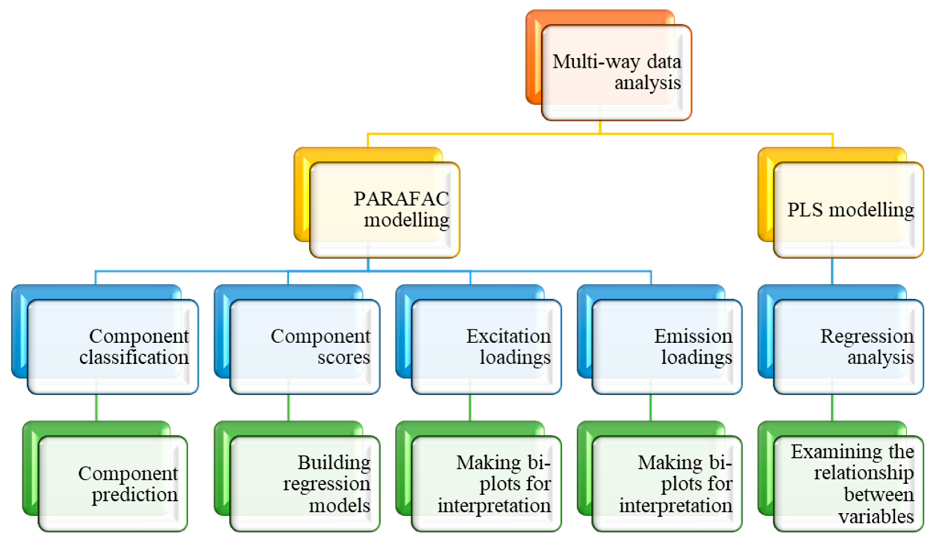
3.8. Multiway Data Analysis
3.8.1. Optimisation of the PARAFAC and PLS Models
3.8.2. Construction of the PARAFAC Model
3.8.3. PARAFAC Model Validation
3.8.4. Construction of the PLS Model
3.8.5. PLS Model Validation
3.8.6. Validation of Spiked Surface Water Samples
3.8.7. Method Sensitivity and Limits of Detection and Quantification
3.8.8. Accuracy and Recovery of the Method
3.8.9. The Robustness of the Model
4. Conclusions
Author Contributions
Funding
Institutional Review Board Statement
Informed Consent Statement
Data Availability Statement
Acknowledgments
Conflicts of Interest
Sample Availability
References
- Iyagawa, S.; Sato, T.; Iguchi, T. Bisphenol A. In Handbook of Hormones; Academic Press: London, UK, 2021; pp. 1003–1004. [Google Scholar]
- Ugoeze, K.C.; Amogu, E.O.; Oluigbo, K.E.; Nwachukwu, N. Environmental and public health impacts of plastic wastes due to healthcare and food products packages: A Review. J. Environ. Sci. Public Health 2021, 5, 1–31. [Google Scholar] [CrossRef]
- Ohore, O.E.; Zhang, S. Endocrine disrupting effects of bisphenol A exposure and recent advances on its removal by water treatment systems. A review. Sci. Afr. 2019, 5, e00135. [Google Scholar] [CrossRef]
- Carabajal, M.D.; Arancibia, J.A.; Escandar, G.M. Excitation-emission fluorescence-kinetic third-order/four-way data: Determination of bisphenol A and nonylphenol in food-contact plastics. Talanta 2019, 197, 348–355. [Google Scholar] [CrossRef]
- Spagnuolo, M.L.; Marini, F.; Sarabia, L.A.; Ortiz, M.C. Migration test of Bisphenol A from polycarbonate cups using excitation-emission fluorescence data with parallel factor analysis. Talanta 2017, 167, 367–378. [Google Scholar] [CrossRef]
- Chen, Y.; Wu, H.L.; Sun, X.D.; Wang, T.; Fang, H.; Chang, Y.Y.; Cheng, L.; Ding, Y.J.; Yu, R.Q. Simultaneous and fast determination of bisphenol A and diphenyl carbonate in polycarbonate plastics by using excitation-emission matrix fluorescence couples with second-order calibration method. Spectrochim. Acta A Mol. Biomol. Spectrosc. 2019, 216, 283–289. [Google Scholar] [CrossRef] [PubMed]
- Booksh, K.S.; Kowalski, B.R. Theory of analytical chemistry. Anal. Chem. 1994, 66, 782A–791A. [Google Scholar] [CrossRef]
- Olivieri, A.C. Analytical advantages of multivariate data processing. One, two, three, infinity? Anal. Chem. 2008, 80, 5713–5720. [Google Scholar] [CrossRef] [PubMed]
- Carter, A.; Joll, C.A. Occurrence and formation of disinfection by-products in the swimming pool environment: A critical review. J. Environ. Sci. 2017, 58, 19–50. [Google Scholar] [CrossRef]
- Bro, R. Multivariate calibration: What is in chemometrics for the analytical chemist? Anal. Chim. Acta 2003, 500, 185–194. [Google Scholar] [CrossRef]
- Gilmore, A.M.; Chen, L. Optical early warning detection of aromatic hydrocarbons in drinking water sources with absorbance, transmission and fluorescence excitation-emission mapping (A-TEEM) instrument technology. In Proceedings of the Next-Generation Spectroscopic Technologies XII, SPIE, Baltimore, MA, USA, 15–17 April 2019; Volume 10983, pp. 45–52. [Google Scholar] [CrossRef]
- Gilmore, A.M.; Horiba Advanced Techno Co Ltd.; Horiba Instruments Inc. Determination of Water Treatment Parameters Based on Absorbance and Fluorescence. U.S. Patent 9,670,072, 21 December 2017. [Google Scholar]
- Klečka, G.M.; Staples, C.A.; Clark, K.E.; Van der Hoeven, N.; Thomas, D.E.; Hentges, S.G. Exposure analysis of bisphenol A in surface water systems in North America and Europe. Environ. Sci. Technol. 2009, 43, 6145–6150. [Google Scholar] [CrossRef] [PubMed]
- Arnold, S.M.; Clark, K.E.; Staples, C.A.; Klecka, G.M.; Dimond, S.S.; Caspers, N.; Hentges, S.G. Relevance of drinking water as a source of human exposure to bisphenol A. J. Exp. Sci. Environ. Epidemiol. 2013, 23, 137–144. [Google Scholar] [CrossRef] [PubMed]
- Wanda, E.; Nyoni, H.; Mamba, B.; Msagati, T. Occurrence of micropollutants in water systems in Guateng, Mpumalanga, and Northwest Provinces, South Africa. Int. J. Environ. Res. Public Health. 2017, 14, 79. [Google Scholar] [CrossRef] [PubMed]
- Zheng, C.; Liu, J.; Ren, J.; Shen, J.; Fan, J.; Xi, R.; Chen, W.; Chen, Q. Occurrence, distribution and ecological risk of bisphenol analogues in the surface water from a water diversion project in Nanjing, China. Int. J. Environ. Res. Public Health 2019, 16, 3296. [Google Scholar] [CrossRef] [PubMed]
- Souza, M.C.O.; Rocha, B.A.; Adeyemi, J.A.; Nadal, M.; Domingo, J.L.; Barbosa, F., Jr. Legacy and emerging pollutants in Latin America: A critical review of occurrence and levels in environmental and food samples. Sci. Total Environ. 2022, 848, 157774. [Google Scholar] [CrossRef]
- Nikolajsen, R.P.H.; Booksh, K.S.; Hansen, A.M.; Bro, R. Quantifying catecholamines using multi-way kinetic modelling. Anal. Chim. Acta 2003, 475, 137–150. [Google Scholar] [CrossRef]
- Bro, R. PARAFAC. Tutorial and applications. Chemom. Intell. Lab. Syst. 1997, 38, 149–171. [Google Scholar] [CrossRef]
- Wold, S.; Sjostrom, M.; Eriksson, L. PLS-regression: A basic tool of chemometrics. Chemom. Intell. Lab. Syst. 2001, 58, 109–130. [Google Scholar] [CrossRef]
- Siqueira, L.F.; Júnior, R.F.A.; de Araújo, A.A.; Morais, C.L.; Lima, K.M. LDA vs. QDA for FT-MIR prostate cancer tissue classification. Chemom. Intell. Lab. Syst. 2017, 162, 123–129. [Google Scholar] [CrossRef]
- Derco, J.; Dudáš, J.; Valičková, M.; Sumegová, L.; Murínová, S. Removal of Alkylphenols from Industrial and Municipal Wastewater. Chem. Biochem. Eng. Q. 2017, 31, 173–178. [Google Scholar] [CrossRef]
- Bocharnikova, E.N.; Tchaikovskaya, O.N.; Bazyl, O.K.; Artyukhov, V.Y.; Mayer, G.V. Theoretical study of bisphenol A photolysis. In Advances in Quantum Chemistry; Academic Press: London, UK, 2020; Volume 81, pp. 191–217. [Google Scholar] [CrossRef]
- Wünsch, U.J.; Murphy, K.R.; Stedmon, C.A. Corrigendum: Fluorescence quantum yields of natural organic matter and organic compounds: Implications for the fluorescence-based interpretation of organic matter composition. Front. Mar. Sci. 2016, 3, 98. [Google Scholar] [CrossRef]
- Xia, Y. Correlation and association analyses in microbiome study integrating multiomics in health and disease. Prog. Mol. Biol. Transl. Sci. 2020, 171, 309–491. [Google Scholar] [CrossRef] [PubMed]
- Hudson, N.; Baker, A.; Reynolds, D. Fluorescence analysis of dissolved organic matter in natural, waste and polluted waters-a review. River Res. Appl. 2007, 23, 631–649. [Google Scholar] [CrossRef]
- Del Olmo, M.; Zafra, A.; Jurado, A.B.; Vilchez, J.L. Determination of bisphenol A (BPA) in the presence of phenol by first-derivative fluorescence following micro liquid-liquid extraction (MLLE). Talanta 2000, 50, 1141–1148. [Google Scholar] [CrossRef] [PubMed]
- Sethuraman, S.; Rajendran, K. Multicharacteristic behavior of tyrosine present in the microdomains of the macromolecule gum arabic at various pH conditions. ACS Omega 2018, 3, 17602–17609. [Google Scholar] [CrossRef] [PubMed]
- Brereton, R.G. Multilevel multifactor designs for multivariate calibration. Analyst 1997, 122, 1521–1529. [Google Scholar] [CrossRef]
- Lia, F.; Formosa, J.P.; Zammit-Mangion, M.; Farrugia, C. The first identification of the uniqueness and authentication of Maltese extra virgin olive oil using 3D-fluorescence spectroscopy coupled with multi-way data analysis. Foods 2020, 9, 498. [Google Scholar] [CrossRef] [PubMed]
- Andersen, C.M.; Bro, R. Practical aspects of PARAFAC modeling of fluorescence excitation-emission data. J. Chemom. 2003, 17, 200–215. [Google Scholar] [CrossRef]
- Halberg, H.F.F.; Bevilacqua, M.; Rinnan, Å. Is core consistency a too conservative diagnostic? J. Chemom. 2023, 37, 1–7. [Google Scholar] [CrossRef]
- Murphy, K.R.; Stedmon, C.A.; Graeber, D.; Bro, R. Fluorescence spectroscopy and multi-way techniques. PARAFAC. Anal. Methods 2013, 5, 6557–6566. [Google Scholar] [CrossRef]
- Sierra, M.M.D.; Giovanela, M.; Parlanti, E.; Soriano-Sierra, E.J. Fluorescence fingerprint of fulvic and humic acids from varied origins as viewed by single-scan and excitation/emission matrix techniques. Chemosphere 2005, 58, 715–733. [Google Scholar] [CrossRef]
- Liu, H.; Pu, Y.; Qiu, X.; Li, B.; Sun, B.; Zhu, X.; Liu, K. Humic Acid Extracts Leading to the Photochemical Bromination of Phenol in Aqueous Bromide Solutions: Influences of Aromatic Components, Polarity and Photochemical Activity. Molecules 2021, 26, 608. [Google Scholar] [CrossRef] [PubMed]
- Hong, Y.J.; Nam, C.J.; Song, K.B.; Cho, G.S.; Uhm, H.S.; Choi, D.I.; Choi, E.H. Measurement of hydroxyl radical density generated from the atmospheric pressure bioplasma jet. J. Instrum. 2012, 7, C03046. [Google Scholar] [CrossRef]
- Polat, E.; Gunay, S. A New Robust Partial Least Squares Regression Method Based on a Robust and an Efficient Adaptive Reweighted Estimator of Covariance. REVSTAT-Stat. J. 2019, 17, 449–474. [Google Scholar] [CrossRef]
- Zhang, Z. Residuals and regression diagnostics: Focusing on logistic regression. Ann. Transl. Med. 2016, 4, 195. [Google Scholar] [CrossRef] [PubMed]
- Xu, T.; Valocchi, A.J. A Bayesian approach to improved calibration and prediction of groundwater models with structural error. Water Resour. Res. 2015, 51, 9290–9311. [Google Scholar] [CrossRef]
- Refat, B.; Yu, P. Evaluation of prediction of indigestible fiber fraction (iNDF) of whole-crop barley silage by using non-destructive spectroscopic techniques as a fast-screening method: Comparison between FTIR vs. NIR. Can. J. Plant Sci. 2022, 102, 1130–1138. [Google Scholar] [CrossRef]
- E2617-17; Standard Practice for Validation of Empirically Derived Multivariate Calibrations Methods. ASTM International: West Conshohocken, PA, USA, 2018. [CrossRef]
- Shen, J.; Valagolam, D.; McCalla, S. Prophet forecasting model: A machine learning approach to predict the concentration of air pollutants (PM2.5, PM10, O3, NO2, SO2, CO) in Seoul, South Korea. PeerJ 2020, 8, e9961. [Google Scholar] [CrossRef] [PubMed]
- Darpo, B.; Nebout, T.; Sager, P.T. Clinical evaluation of QT/QTc prolongation and proarrhythmic potential for nonantiarrhythmic drugs: The International Conference on Harmonization of Technical Requirements for Registration of Pharmaceuticals for Human Use E14 guideline. J. Clin. Pharmacol. 2006, 46, 498–507. [Google Scholar] [CrossRef] [PubMed]
- Zulfikar, R. Estimation Model and Selection Method of Panel Data Regression: An Overview of Common Effect, Fixed Effect, and Random Effect Model, INA-Rxiv 9qe2b; Center for Open Science: Charlottesville, VA, USA, 2019; pp. 1–10. [Google Scholar]
- Ziliak, S. P values and the search for significance. Nat. Methods 2017, 14, 3–4. [Google Scholar]
- Radu, E.; Stoica, R.; Calin, C.; Oprescu, E.E.; Bolocan, I.; Ion, I.; Ion, A.C. Validation of a RP-HPLC-UV method for the determination of bisphenol A at low levels in natural mineral water. Rev. Chim. 2016, 67, 230–240. [Google Scholar]
- Kianpoor Kalkhajeh, Y.; Jabbarian Amiri, B.; Huang, B.; Henareh Khalyani, A.; Hu, W.; Gao, H.; Thompson, M.L. Methods for sample collection, storage, and analysis of freshwater phosphorus. Water 2019, 11, 1889. [Google Scholar] [CrossRef]
- Biau, D.J.; Kernéis, S.; Porcher, R. Statistics in brief: The importance of sample size in the planning and interpretation of medical research. Clin. Orthop. Relat. Res. 2008, 466, 2282–2288. [Google Scholar] [CrossRef] [PubMed]
- Mundfrom, D.J.; Shaw, D.G.; Ke, T.L. Minimum sample size recommendations for conducting factor analyses. Int. J. Test. 2005, 5, 159–168. [Google Scholar] [CrossRef]
- Subasi, A. Practical Machine Learning for Data Analysis Using Python; Academic Press: Cambridge, MA, USA, 2020; pp. 1–524. [Google Scholar] [CrossRef]
- Bro, R.; Kiers, H.A. A new efficient method for determining the number of components in PARAFAC models. J. Chemom. 2003, 17, 274–286. [Google Scholar] [CrossRef]
- Stedmon, C.A.; Bro, R. Characterizing dissolved organic matter fluorescence with parallel factor analysis: A tutorial. Limnol. Oceanogr. Meth. 2008, 6, 572–579. [Google Scholar] [CrossRef]
- Gautam, R.; Vanga, S.; Ariese, F.; Umapathy, S. Review of multidimensional data processing approaches for Raman and infrared spectroscopy. EPJ Tech. Instrum. 2015, 2, 8. [Google Scholar] [CrossRef]
- Deng, B.C.; Yun, Y.H.; Liang, Y.Z.; Cao, D.S.; Xu, Q.S.; Yi, L.Z.; Huang, X. A new strategy to prevent over-fitting in partial least squares models based on model population analysis. Anal. Chim. Acta 2015, 880, 32–41. [Google Scholar] [CrossRef] [PubMed]
- Rinnan, A.; Andersson, M.; Ridder, C.; Engelsen, S.B. Recursive weighted partial least squares (rPLS): An efficient variable selection method using PLS. J. Chemom. 2014, 28, 439–447. [Google Scholar] [CrossRef]
- Häggblom, K.E. Basics of Multivariate Modelling and Data Analysis. Disponible en. 2018. Available online: http://www.users.abo.fi/khaggblo/MMDA/MMDA6.pdf (accessed on 13 September 2022).
- Sarigiannis, D.; Parnell, T.; Pozidis, H. Weighted sampling for combined model selection and hyperparameter tuning. In Proceedings of the AAAI Conference on Artificial Intelligence, New York, NY, USA, 7–12 February 2020; Volume 34, pp. 5595–5603. [Google Scholar] [CrossRef]
- Chen, J.; LeBoeuf, E.J.; Dai, S.; Gu, B. Fluorescence spectroscopic studies of natural organic matter fractions. Chemosphere 2003, 50, 639–647. [Google Scholar] [CrossRef] [PubMed]
- Steiner, D.; Krska, R.; Malachová, A.; Taschl, I.; Sulyok, M. Evaluation of matrix effects and extraction efficiencies of LC–MS/MS methods as the essential part for proper validation of multiclass contaminants in complex feed. J. Agric. Food Chem. 2020, 68, 3868–3880. [Google Scholar] [CrossRef]
- Sanco, D.G. Method Validation and Quality Control Procedures for Pesticide Residues Analysis in Food and Feed; Document No. SANCO/12495/2011l European Commission. 2013. Available online: www.crl-pesticides.eu/library/docs/fv/SANCO12495-2011.pdf (accessed on 13 September 2023).


| Chemical structure | 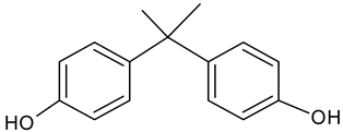 |
| Molecular formula, molecular weight | C15H16O2, 228.291 |
| CAS number | 80-05-7 |
| Parameter | Value |
|---|---|
| Number of LVs | 5 |
| RMSEC (µM) | 17.434 |
| RMSECV (µM) | 34.794 |
| Calibration Bias | 1.396 |
| CV Bias | 0.33 |
| R2 for Calibration | 0.967 |
| R2 for Cross-Validation | 0.845 |
| Parameter | Value |
|---|---|
| Residual sum of squares | 97.311 |
| Pearson’s r | 0.998 |
| R-Squared (COD) | 0.996 |
| Adj. R-squared | 0.996 |
| RMSE | 5.272 |
| MAE | 4.378 |
| Intercept | 4.219 |
| Standard error of intercept | 3.079 |
| Slope | 0.98 |
| Standard error of slope | 0.0167 |
| Degrees of Freedom | Sum of Squares | Mean Squares | F Value | Prob > F | |
|---|---|---|---|---|---|
| Model | 1 | 95,914.648 | 95,914.648 | 210.474 | 0 |
| Error | 14 | 389.073 | 27.791 | ||
| Total | 15 | 96,303.722 |
| Nominal Conc. of BPA (µM) | Measured Conc. of BPA (µM) | Percent Recovery |
|---|---|---|
| 50 | 47.715 | 95.43 |
| 180 | 178.686 | 99.27 |
| 270 | 264.465 | 97.95 |
Disclaimer/Publisher’s Note: The statements, opinions and data contained in all publications are solely those of the individual author(s) and contributor(s) and not of MDPI and/or the editor(s). MDPI and/or the editor(s) disclaim responsibility for any injury to people or property resulting from any ideas, methods, instructions or products referred to in the content. |
© 2023 by the authors. Licensee MDPI, Basel, Switzerland. This article is an open access article distributed under the terms and conditions of the Creative Commons Attribution (CC BY) license (https://creativecommons.org/licenses/by/4.0/).
Share and Cite
Ingwani, T.; Chaukura, N.; Mamba, B.B.; Nkambule, T.T.I.; Gilmore, A.M. Detection and Quantification of Bisphenol A in Surface Water Using Absorbance–Transmittance and Fluorescence Excitation–Emission Matrices (A-TEEM) Coupled with Multiway Techniques. Molecules 2023, 28, 7048. https://doi.org/10.3390/molecules28207048
Ingwani T, Chaukura N, Mamba BB, Nkambule TTI, Gilmore AM. Detection and Quantification of Bisphenol A in Surface Water Using Absorbance–Transmittance and Fluorescence Excitation–Emission Matrices (A-TEEM) Coupled with Multiway Techniques. Molecules. 2023; 28(20):7048. https://doi.org/10.3390/molecules28207048
Chicago/Turabian StyleIngwani, Thomas, Nhamo Chaukura, Bhekie B. Mamba, Thabo T. I. Nkambule, and Adam M. Gilmore. 2023. "Detection and Quantification of Bisphenol A in Surface Water Using Absorbance–Transmittance and Fluorescence Excitation–Emission Matrices (A-TEEM) Coupled with Multiway Techniques" Molecules 28, no. 20: 7048. https://doi.org/10.3390/molecules28207048