Visual Head Counts: A Promising Method for Efficient Monitoring of Diamondback Terrapins


Abstract
:1. Introduction
2. Materials and Methods
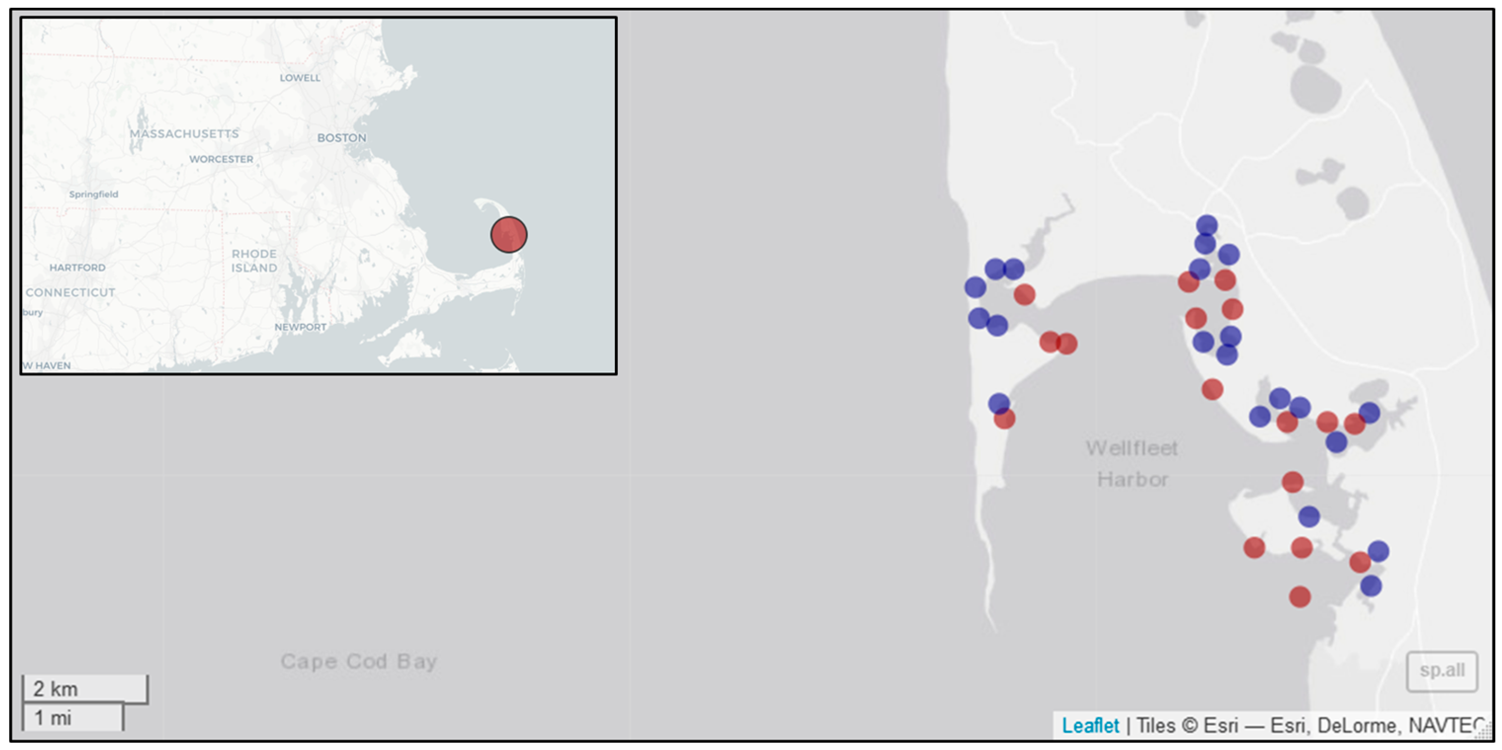
2.1. Study Area
2.2. Visual Head Count Surveys
2.3. Statistical Analysis
3. Results
4. Discussion
5. Conclusions
Author Contributions
Funding
Acknowledgments
Conflicts of Interest
Appendix A

| Negative Binomial | Poisson | ||||||||||
|---|---|---|---|---|---|---|---|---|---|---|---|
| Detection | Abundance | K | AIC | ΔAIC | ωAIC | ΣωAIC | K | AIC | ΔAIC | ωAIC | ΣωAIC |
| p(wind + airtemp + expo) | λ(relday × expo) | 9 | 2442.84 | 0.00 | 0.33 | 0.33 | 8 | 4257.74 | 1814.89 | 0.00 | 1.00 |
| p(wind + airtemp + expo) | λ(relday) | 7 | 2443.66 | 0.81 | 0.22 | 0.56 | 6 | 4294.18 | 1851.33 | 0.00 | 1.00 |
| p(wind + airtemp + expo) | λ(relday + expo) | 8 | 2444.29 | 1.44 | 0.16 | 0.72 | 7 | 4272.59 | 1829.75 | 0.00 | 1.00 |
| p(wind + ccov + airtemp + expo) | λ(relday × expo) | 13 | 2444.85 | 2.00 | 0.12 | 0.84 | 12 | 4200.42 | 1757.57 | 0.00 | 1.00 |
| p(wind + ccov + airtemp + expo) | λ(relday) | 11 | 2447.12 | 4.28 | 0.04 | 0.88 | 10 | 4257.23 | 1814.39 | 0.00 | 1.00 |
| p(wind + airtemp) | λ(relday × expo) | 8 | 2447.34 | 4.50 | 0.04 | 0.92 | 7 | 4314.40 | 1871.55 | 0.00 | 1.00 |
| p(wind + ccov + airtemp) | λ(relday × expo) | 12 | 2447.66 | 4.81 | 0.03 | 0.95 | 11 | 4222.54 | 1779.70 | 0.00 | 1.00 |
| p(wind + ccov + airtemp + expo) | λ(relday + expo) | 12 | 2447.90 | 5.05 | 0.03 | 0.98 | 11 | 4227.21 | 1784.36 | 0.00 | 1.00 |
| p(wind + airtemp) | λ(relday + expo) | 7 | 2449.37 | 6.53 | 0.01 | 0.99 | 6 | 4346.61 | 1903.77 | 0.00 | 1.00 |
| p(wind + ccov + airtemp) | λ(relday + expo) | 11 | 2450.90 | 8.05 | 0.01 | 0.99 | 10 | 4265.13 | 1822.28 | 0.00 | 1.00 |
| p(wind + ccov + expo) | λ(relday × expo) | 12 | 2454.49 | 11.65 | 0.00 | 1.00 | 11 | 4231.32 | 1788.48 | 0.00 | 1.00 |
| p(wind + ccov) | λ(relday × expo) | 11 | 2454.71 | 11.87 | 0.00 | 1.00 | 10 | 4240.50 | 1797.66 | 0.00 | 1.00 |
| p(wind + ccov + airtemp) | λ(relday) | 10 | 2454.88 | 12.03 | 0.00 | 1.00 | 9 | 4425.24 | 1982.39 | 0.00 | 1.00 |
| p(airtemp + expo) | λ(relday × expo) | 8 | 2456.70 | 13.86 | 0.00 | 1.00 | 7 | 4326.87 | 1884.03 | 0.00 | 1.00 |
| p(wind + ccov + expo) | λ(relday) | 10 | 2456.70 | 13.86 | 0.00 | 1.00 | 9 | 4352.01 | 1909.16 | 0.00 | 1.00 |
| p(wind + airtemp) | λ(relday) | 6 | 2456.77 | 13.92 | 0.00 | 1.00 | 5 | 4506.19 | 2063.34 | 0.00 | 1.00 |
| p(ccov + airtemp + expo) | λ(relday × expo) | 12 | 2457.24 | 14.40 | 0.00 | 1.00 | 11 | 4259.03 | 1816.18 | 0.00 | 1.00 |
| p(airtemp + expo) | λ(relday) | 6 | 2457.40 | 14.55 | 0.00 | 1.00 | 5 | 4374.93 | 1932.09 | 0.00 | 1.00 |
| p(airtemp + expo) | λ(relday + expo) | 7 | 2457.67 | 14.83 | 0.00 | 1.00 | 6 | 4344.72 | 1901.87 | 0.00 | 1.00 |
| p(wind + ccov + expo) | λ(relday + expo) | 11 | 2458.35 | 15.51 | 0.00 | 1.00 | 10 | 4269.38 | 1826.54 | 0.00 | 1.00 |
| p(wind + ccov) | λ(relday + expo) | 10 | 2458.36 | 15.51 | 0.00 | 1.00 | 9 | 4278.68 | 1835.83 | 0.00 | 1.00 |
| p(wind + airtemp + expo) | λ(∙) | 6 | 2458.46 | 15.61 | 0.00 | 1.00 | 5 | 4483.82 | 2040.97 | 0.00 | 1.00 |
| p(ccov + airtemp + expo) | λ(relday) | 10 | 2458.69 | 15.85 | 0.00 | 1.00 | 9 | 4326.81 | 1883.97 | 0.00 | 1.00 |
| p(ccov + airtemp + expo) | λ(relday + expo) | 11 | 2459.79 | 16.94 | 0.00 | 1.00 | 10 | 4285.82 | 1842.98 | 0.00 | 1.00 |
| p(wind) | λ(relday × expo) | 7 | 2460.12 | 17.28 | 0.00 | 1.00 | 6 | 4369.22 | 1926.37 | 0.00 | 1.00 |
| p(wind + airtemp + expo) | λ(expo) | 7 | 2460.28 | 17.44 | 0.00 | 1.00 | 6 | 4428.94 | 1986.09 | 0.00 | 1.00 |
| p(wind + expo) | λ(relday × expo) | 8 | 2460.46 | 17.62 | 0.00 | 1.00 | 7 | 4348.12 | 1905.28 | 0.00 | 1.00 |
| p(ccov + airtemp) | λ(relday × expo) | 11 | 2460.48 | 17.63 | 0.00 | 1.00 | 10 | 4295.68 | 1852.83 | 0.00 | 1.00 |
| p(wind + ccov + airtemp + expo) | λ(∙) | 10 | 2461.39 | 18.55 | 0.00 | 1.00 | 9 | 4435.15 | 1992.31 | 0.00 | 1.00 |
| p(wind + ccov) | λ(relday) | 9 | 2461.40 | 18.56 | 0.00 | 1.00 | 8 | 4433.07 | 1990.22 | 0.00 | 1.00 |
| p(wind + expo) | λ(relday) | 6 | 2461.52 | 18.68 | 0.00 | 1.00 | 5 | 4462.58 | 2019.74 | 0.00 | 1.00 |
| p(wind + ccov + expo) | λ(∙) | 9 | 2462.22 | 19.37 | 0.00 | 1.00 | 8 | 4444.15 | 2001.31 | 0.00 | 1.00 |
| p(wind + airtemp) | λ(expo) | 6 | 2462.84 | 19.99 | 0.00 | 1.00 | 5 | 4476.29 | 2033.45 | 0.00 | 1.00 |
| p(ccov + airtemp) | λ(relday + expo) | 10 | 2463.17 | 20.32 | 0.00 | 1.00 | 9 | 4338.50 | 1895.65 | 0.00 | 1.00 |
| p(wind) | λ(relday + expo) | 6 | 2463.20 | 20.35 | 0.00 | 1.00 | 5 | 4397.94 | 1955.09 | 0.00 | 1.00 |
| p(wind + ccov + airtemp + expo) | λ(expo) | 11 | 2463.21 | 20.36 | 0.00 | 1.00 | 10 | 4368.54 | 1925.70 | 0.00 | 1.00 |
| p(wind + expo) | λ(relday + expo) | 7 | 2463.51 | 20.66 | 0.00 | 1.00 | 6 | 4376.51 | 1933.67 | 0.00 | 1.00 |
| p(wind + ccov) | λ(expo) | 9 | 2464.18 | 21.34 | 0.00 | 1.00 | 8 | 4382.69 | 1939.85 | 0.00 | 1.00 |
| p(wind + ccov + expo) | λ(expo) | 10 | 2464.21 | 21.36 | 0.00 | 1.00 | 9 | 4367.07 | 1924.22 | 0.00 | 1.00 |
| p(airtemp) | λ(relday x expo) | 7 | 2464.22 | 21.38 | 0.00 | 1.00 | 6 | 4411.12 | 1968.28 | 0.00 | 1.00 |
| p(wind + ccov + airtemp) | λ(expo) | 10 | 2464.36 | 21.52 | 0.00 | 1.00 | 9 | 4383.33 | 1940.49 | 0.00 | 1.00 |
| p(wind + expo) | λ(∙) | 5 | 2465.54 | 22.70 | 0.00 | 1.00 | 4 | 4542.02 | 2099.18 | 0.00 | 1.00 |
| p(airtemp) | λ(relday + expo) | 6 | 2465.99 | 23.15 | 0.00 | 1.00 | 5 | 4447.64 | 2004.79 | 0.00 | 1.00 |
| p(wind) | λ(expo) | 5 | 2466.74 | 23.89 | 0.00 | 1.00 | 4 | 4478.46 | 2035.61 | 0.00 | 1.00 |
| p(wind + expo) | λ(expo) | 6 | 2466.99 | 24.14 | 0.00 | 1.00 | 5 | 4452.53 | 2009.69 | 0.00 | 1.00 |
| p(airtemp + expo) | λ(∙) | 5 | 2469.20 | 26.35 | 0.00 | 1.00 | 4 | 4538.96 | 2096.12 | 0.00 | 1.00 |
| p(wind) | λ(relday) | 5 | 2469.22 | 26.38 | 0.00 | 1.00 | 4 | 4556.42 | 2113.57 | 0.00 | 1.00 |
| p(ccov + airtemp) | λ(relday) | 9 | 2469.49 | 26.64 | 0.00 | 1.00 | 8 | 4517.83 | 2074.98 | 0.00 | 1.00 |
| p(ccov + expo) | λ(relday × expo) | 11 | 2469.57 | 26.73 | 0.00 | 1.00 | 10 | 4319.56 | 1876.71 | 0.00 | 1.00 |
| p(ccov) | λ(relday × expo) | 10 | 2470.03 | 27.18 | 0.00 | 1.00 | 9 | 4341.84 | 1899.00 | 0.00 | 1.00 |
| p(airtemp + expo) | λ(expo) | 6 | 2470.97 | 28.12 | 0.00 | 1.00 | 5 | 4477.94 | 2035.10 | 0.00 | 1.00 |
| p(ccov + expo) | λ(relday) | 9 | 2471.48 | 28.64 | 0.00 | 1.00 | 8 | 4458.38 | 2015.53 | 0.00 | 1.00 |
| p(wind + ccov) | λ(∙) | 8 | 2472.54 | 29.69 | 0.00 | 1.00 | 7 | 4539.74 | 2096.90 | 0.00 | 1.00 |
| p(ccov + airtemp + expo) | λ(∙) | 9 | 2473.24 | 30.40 | 0.00 | 1.00 | 8 | 4502.02 | 2059.18 | 0.00 | 1.00 |
| p(expo) | λ(relday × expo) | 7 | 2473.30 | 30.46 | 0.00 | 1.00 | 6 | 4409.04 | 1966.20 | 0.00 | 1.00 |
| p(ccov + expo) | λ(relday + expo) | 10 | 2473.47 | 30.63 | 0.00 | 1.00 | 9 | 4358.68 | 1915.83 | 0.00 | 1.00 |
| p(ccov) | λ(relday + expo) | 9 | 2473.60 | 30.76 | 0.00 | 1.00 | 8 | 4381.27 | 1938.43 | 0.00 | 1.00 |
| p(expo) | λ(relday) | 5 | 2473.83 | 30.98 | 0.00 | 1.00 | 4 | 4538.54 | 2095.69 | 0.00 | 1.00 |
| p(wind + ccov + airtemp) | λ(∙) | 9 | 2474.03 | 31.19 | 0.00 | 1.00 | 8 | 4540.46 | 2097.62 | 0.00 | 1.00 |
| p(∙) | λ(relday × expo) | 6 | 2474.31 | 31.47 | 0.00 | 1.00 | 5 | 4457.35 | 2014.50 | 0.00 | 1.00 |
| p(ccov + airtemp + expo) | λ(expo) | 10 | 2475.23 | 32.38 | 0.00 | 1.00 | 9 | 4433.41 | 1990.57 | 0.00 | 1.00 |
| p(expo) | λ(relday + expo) | 6 | 2475.77 | 32.93 | 0.00 | 1.00 | 5 | 4439.17 | 1996.33 | 0.00 | 1.00 |
| p(airtemp) | λ(expo) | 5 | 2476.09 | 33.24 | 0.00 | 1.00 | 4 | 4554.15 | 2111.30 | 0.00 | 1.00 |
| p(wind + airtemp) | λ(∙) | 5 | 2476.26 | 33.42 | 0.00 | 1.00 | 4 | 4640.62 | 2197.78 | 0.00 | 1.00 |
| p(∙) | λ(relday + expo) | 5 | 2476.82 | 33.98 | 0.00 | 1.00 | 4 | 4486.70 | 2043.86 | 0.00 | 1.00 |
| p(airtemp) | λ(relday) | 5 | 2476.85 | 34.00 | 0.00 | 1.00 | 4 | 4629.31 | 2186.46 | 0.00 | 1.00 |
| p(ccov + airtemp) | λ(expo) | 9 | 2476.89 | 34.04 | 0.00 | 1.00 | 8 | 4475.53 | 2032.69 | 0.00 | 1.00 |
| p(ccov + expo) | λ(∙) | 8 | 2476.97 | 34.12 | 0.00 | 1.00 | 7 | 4539.94 | 2097.10 | 0.00 | 1.00 |
| p(expo) | λ(∙) | 4 | 2477.26 | 34.42 | 0.00 | 1.00 | 3 | 4605.42 | 2162.58 | 0.00 | 1.00 |
| p(wind) | λ(∙) | 4 | 2477.41 | 34.56 | 0.00 | 1.00 | 3 | 4644.02 | 2201.18 | 0.00 | 1.00 |
| p(ccov + expo) | λ(expo) | 9 | 2478.54 | 35.70 | 0.00 | 1.00 | 8 | 4447.38 | 2004.54 | 0.00 | 1.00 |
| p(expo) | λ(expo) | 5 | 2478.54 | 35.70 | 0.00 | 1.00 | 4 | 4506.40 | 2063.55 | 0.00 | 1.00 |
| p(ccov) | λ(expo) | 8 | 2478.59 | 35.75 | 0.00 | 1.00 | 7 | 4477.81 | 2034.97 | 0.00 | 1.00 |
| p(ccov) | λ(relday) | 8 | 2479.50 | 36.66 | 0.00 | 1.00 | 7 | 4550.86 | 2108.02 | 0.00 | 1.00 |
| p(∙) | λ(expo) | 4 | 2479.64 | 36.79 | 0.00 | 1.00 | 3 | 4558.73 | 2115.88 | 0.00 | 1.00 |
| p(∙) | λ(relday) | 4 | 2486.83 | 43.99 | 0.00 | 1.00 | 3 | 4648.64 | 2205.80 | 0.00 | 1.00 |
| p(ccov) | λ(∙) | 7 | 2490.58 | 47.74 | 0.00 | 1.00 | 6 | 4647.29 | 2204.45 | 0.00 | 1.00 |
| p(ccov + airtemp) | λ(∙) | 8 | 2490.62 | 47.77 | 0.00 | 1.00 | 7 | 4645.78 | 2202.94 | 0.00 | 1.00 |
| p(airtemp) | λ(∙) | 4 | 2493.26 | 50.42 | 0.00 | 1.00 | 3 | 4722.14 | 2279.29 | 0.00 | 1.00 |
| p(∙) | λ(∙) | 3 | 2494.67 | 51.83 | 0.00 | 1.00 | 2 | 4725.64 | 2282.80 | 0.00 | 1.00 |
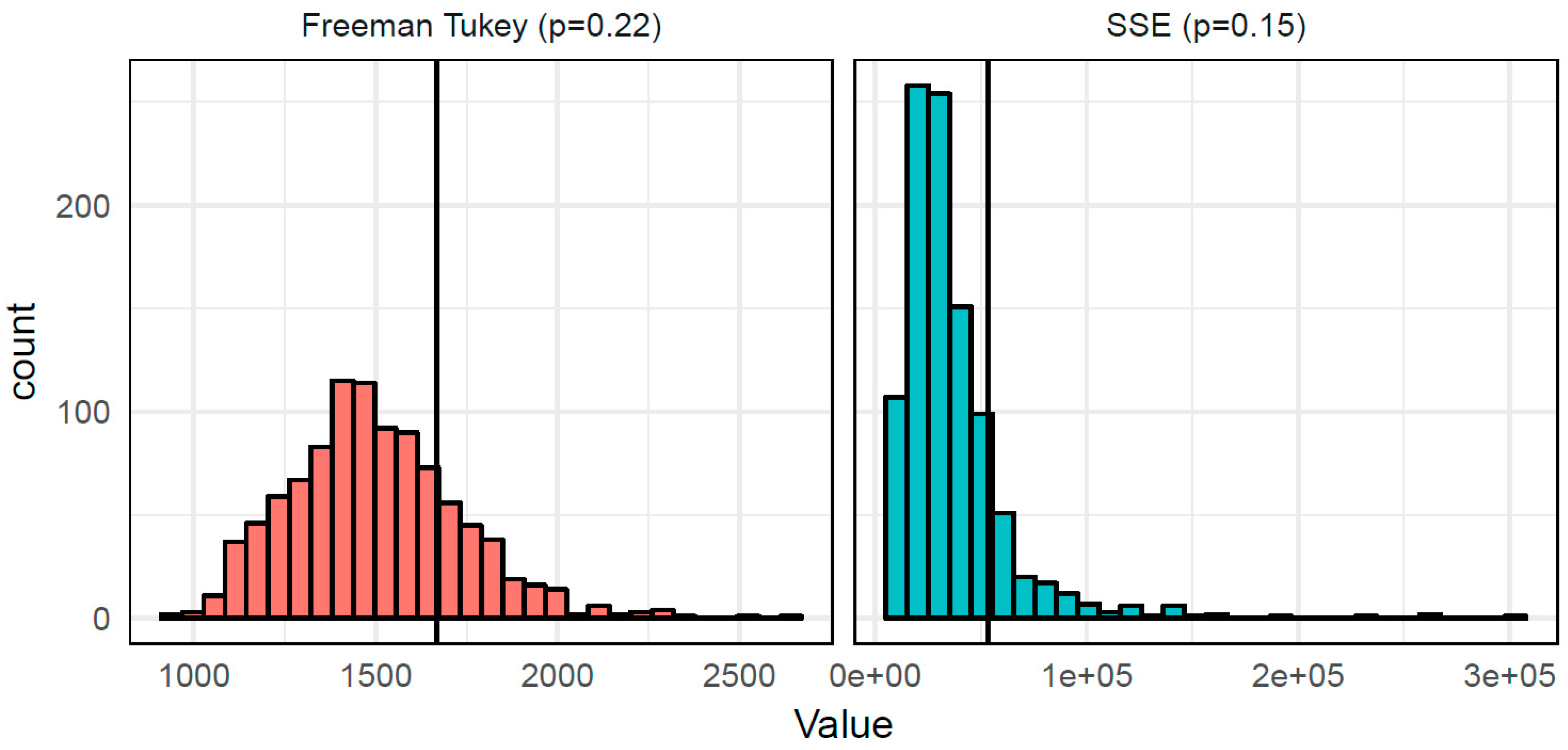
| Test Statistic | θobs | Mean(θobs − θboot) | SD(θobs − θboot) | Pr(θboot > θobs) |
|---|---|---|---|---|
| SSE | 53,435 | 16,737 | 26,883 | 0.153 |
| Freeman Tukey | 1667 | 169 | 236 | 0.215 |

References
- Hart, K.M.; Lee, D.S. The diamondback terrapin: The biology, ecology, cultural history, and conservation status of an obligate estuarine turtle. Stud. Avian. Biol. 2006. [Google Scholar] [CrossRef]
- Ernst, C.M.; Lovich, J.E. Turtles of the United States and Canada, 2nd ed.; The John Hopkins University Press: Baltimore, MD, USA, 2009. [Google Scholar]
- Roosenburg, W.M.; Kennedy, V.S. Ecology and Conservation of the Diamond-backed Terrapin; John Hopkins University Press: Baltimore, MD, USA, 2018. [Google Scholar]
- Harden, L.A.; Pittman, S.E.; Gibbons, J.W.; Dorcas, M.E. Development of a rapid-assessment technique for diamondback terrapin (Malaclemys terrapin) populations using head-count surveys. Appl. Herpetol. 2009. [Google Scholar] [CrossRef]
- Duncan, A.N.P.; Burke, R.L. Dispersal of Newly Emerged Diamond-Backed Terrapin (Malaclemys terrapin) Hatchlings at Jamaica Bay, New York. Chelonian Conserv. Biol. 2016, 15, 249–256. [Google Scholar] [CrossRef]
- Seigel, R.A. Courtship and Mating Behavior of the Diamondback Terrapin Malaclemys terrapin tequesta. J. Herpetol. 1980, 14, 420–421. [Google Scholar] [CrossRef]
- Brennessel, B. Diamonds in The Marsh: A Natural History of the Diamondback Terrapin; University Press of New England: Lebanon, NH, USA, 2006. [Google Scholar]
- Baker, P.J.; Thomson, A.; Vatnick, I.; Wood, R.C. Estimating survival times for northern diamondback terrapins, Malaclemys terrapin terrapin, in submerged crab pots. Herpetol. Conserv. Biol. 2013, 8, 667–680. [Google Scholar]
- Butler, J.A. Population Ecology, Home Range, and Seasonal Movements of the Carolina Diamondback Terrapin, Malaclemys terrapin centrata, in Northeastern Florida; Florida Fish and Wildlife Conservation Commission: Tallahassee, FL, USA, 2002. [Google Scholar]
- Hart, K.M.; McIvor, C.C. Demography and Ecology of Mangrove Diamondback Terrapins in a Wilderness Area of Everglades National Park, Florida, USA. Copeia 2008, 2008, 200–208. [Google Scholar] [CrossRef]
- Baxter, A.S.; Hill, E.M.; Withers, K. Population assessment of texas diamondback terrapin. Texas J. Sci. 2016, 65, 51–63. [Google Scholar]
- Simoes, J.C.; Chambers, R.M. The Diamondback Terrapins of Piermont Marsh, Hudson River, New York. Northeast. Nat. 1999, 6, 241–248. [Google Scholar] [CrossRef]
- Butler, J.A. Status and Distribution of the Carolina Diamondback Terrapin, Malaclemys terrapin centrata, in Duval County; Florida Fish and Wildlife Conservation Commission: Tallahassee, FL, USA, 2000; p. 52. [Google Scholar]
- Akins, C.D.; Ruder, C.D.; Price, S.J.; Harden, L.A.; Gibbons, J.W.; Dorcas, M.E. Factors affecting temperature variation and habitat use in free-ranging diamondback terrapins. J. Therm. Biol. 2014, 44, 63–69. [Google Scholar] [CrossRef] [PubMed]
- Selman, W.; Baccigalopi, B.; Baccigalopi, C. Distribution and Abundance of Diamondback Terrapins (Malaclemys terrapin) in Southwestern Louisiana. Chelonian Conserv. Biol. 2014, 13, 131–139. [Google Scholar] [CrossRef]
- Henry, P.F.P.; Haramis, G.M.; Day, D.D. Evaluating a portable cylindrical bait trap to capture diamondback terrapins in salt marsh. Wildl. Soc. Bull. 2016, 40, 160–168. [Google Scholar] [CrossRef]
- Byers, J.E.; Altman, I.; Grosse, A.M.; Huspeni, T.C.; Maerz, J.C. Using Parasitic Trematode Larvae to Quantify an Elusive Vertebrate Host. Conserv. Biol. 2011, 25, 85–93. [Google Scholar] [CrossRef] [PubMed]
- King, P.; Ludlam, J.P. Status of Diamondback Terrapins (Malaclemys terrapin) in North Inlet–Winyah Bay, South Carolina. Chelonian Conserv. Biol. 2014, 13, 119–124. [Google Scholar] [CrossRef]
- Mass Audubon. Wellfleet Bay Wildlife Sanctuary Diamondback Terrapins [Internet]; Mass Audubon: Lincoln, MA, USA, 2019; Available online: https://www.massaudubon.org/get-outdoors/wildlife-sanctuaries/wellfleet-bay/about/our-conservation-work/diamondback-terrapins (accessed on 10 January 2019).
- Kanonik, A.; Burke, R.; Burke, R.L. Demographic Analysis of the Jamaica Bay Diamondback Terrapin Population: Implications for Survival in an Urban Habitat. Available online: http://www.hudsonriver.org/ls/reports/Polgar_Kanonik_TP_05_09_final.pdf (accessed on 10 January 2019).
- Roosenburg, W.M. Final Report Chesapeake Diamondback Terrapin Investigations for the Period 1987, 1988, and 1989; Chesapeake Research Consortium: Solomons, MD, USA, 1990. [Google Scholar]
- Isdell, R.E.; Chambers, R.M.; Bilkovic, D.M.; Leu, M. Effects of terrestrial-aquatic connectivity on an estuarine turtle. Divers. Distrib. 2015, 21, 643–653. [Google Scholar] [CrossRef]
- Ralph, C.J.; Sauer, J.R.; Droege, S. Monitoring Bird Populations by Point Counts. 1995. Available online: https://www.fs.fed.us/psw/publications/documents/psw_gtr149/psw_gtr149.pdf (accessed on 9 March 2019).
- Royle, J.A. N-Mixture Models for Estimating Population Size from Spatially Replicated Counts. Biometrics 2004, 60, 108–115. [Google Scholar] [CrossRef] [PubMed]
- Kéry, M.; Royle, J.A. Applied Hierarchical Modeling in Ecology: Analysis of Distribution, Abundance and Species Richness in R and BUGS: Volume 1: Prelude and Static Models; Academic Press: San Diego, CA, USA, 2015. [Google Scholar]
- Royle, J.A.; Dorazio, R.M. Hierarchical Modeling and Inference in Ecology: The Analysis of Data from Populations, Metapopulations and Communities; Academic Press: Oxford, UK, 2008. [Google Scholar]
- Fiske, I.J.; Chandler, R.B. Unmarked: An R package for fitting hierarchical models of wildlife occurrence and abundance. J. Stat. Softw. 2011, 43, 1–23. [Google Scholar] [CrossRef]
- Burnham, K.P.; Anderson, D.R. Model Selection and Multimodel Inference: A Practical Information-Theoretic Approach; Springer: New York, NY, USA, 2002. [Google Scholar]
- Arnold, T.W. Uninformative Parameters and Model Selection Using Akaike’s Information Criterion. J. Wildl. Manag. 2010, 74, 1175–1178. [Google Scholar] [CrossRef]
- Knape, J.; Arlt, D.; Barraquand, F.; Berg, Å.; Chevalier, M.; Pärt, T.; Ruete, A.; Żmihorski, M. Sensitivity of binomial N-mixture models to overdispersion: The importance of assessing model fit. Methods Ecol. Evol. 2018, 9, 2102–2114. [Google Scholar] [CrossRef]


| Detection | Abundance | K | AIC | ΔAIC | ωAIC | ΣωAIC |
|---|---|---|---|---|---|---|
| p(wind + airtemp + expo) | λ(relday × expo) | 9 | 2442.84 | 0.00 | 0.33 | 0.33 |
| p(wind + airtemp + expo) | λ(relday) | 7 | 2443.66 | 0.81 | 0.22 | 0.56 |
| p(wind + airtemp + expo) | λ(relday + expo) | 8 | 2444.29 | 1.44 | 0.16 | 0.72 |
| p(wind + ccov + airtemp + expo) | λ(relday × expo) | 13 | 2444.85 | 2.00 | 0.12 | 0.84 |
| p(wind + ccov + airtemp + expo) | λ(relday) | 11 | 2447.12 | 4.28 | 0.04 | 0.88 |
| p(wind + airtemp) | λ(relday × expo) | 8 | 2447.34 | 4.50 | 0.04 | 0.92 |
| p(wind + ccov + airtemp) | λ(relday × expo) | 12 | 2447.66 | 4.81 | 0.03 | 0.95 |
| p(wind + ccov + airtemp + expo) | λ(relday + expo) | 12 | 2447.90 | 5.05 | 0.03 | 0.98 |
| p(wind + airtemp) | λ(relday + expo) | 7 | 2449.37 | 6.53 | 0.01 | 0.99 |
| p(wind + ccov + airtemp) | λ(relday + expo) | 11 | 2450.90 | 8.05 | 0.01 | 0.99 |
© 2019 by the authors. Licensee MDPI, Basel, Switzerland. This article is an open access article distributed under the terms and conditions of the Creative Commons Attribution (CC BY) license (http://creativecommons.org/licenses/by/4.0/).
Share and Cite
Levasseur, P.; Sterrett, S.; Sutherland, C. Visual Head Counts: A Promising Method for Efficient Monitoring of Diamondback Terrapins. Diversity 2019, 11, 101. https://doi.org/10.3390/d11070101
Levasseur P, Sterrett S, Sutherland C. Visual Head Counts: A Promising Method for Efficient Monitoring of Diamondback Terrapins. Diversity. 2019; 11(7):101. https://doi.org/10.3390/d11070101
Chicago/Turabian StyleLevasseur, Patricia, Sean Sterrett, and Chris Sutherland. 2019. "Visual Head Counts: A Promising Method for Efficient Monitoring of Diamondback Terrapins" Diversity 11, no. 7: 101. https://doi.org/10.3390/d11070101
APA StyleLevasseur, P., Sterrett, S., & Sutherland, C. (2019). Visual Head Counts: A Promising Method for Efficient Monitoring of Diamondback Terrapins. Diversity, 11(7), 101. https://doi.org/10.3390/d11070101