Using Maximum Entropy Modeling for Optimal Selection of Sampling Sites for Monitoring Networks

Abstract
: Environmental monitoring programs must efficiently describe state shifts. We propose using maximum entropy modeling to select dissimilar sampling sites to capture environmental variability at low cost, and demonstrate a specific application: sample site selection for the Central Plains domain (453,490 km2) of the National Ecological Observatory Network (NEON). We relied on four environmental factors: mean annual temperature and precipitation, elevation, and vegetation type. A “sample site” was defined as a 20 km × 20 km area (equal to NEON's airborne observation platform [AOP] footprint), within which each 1 km2 cell was evaluated for each environmental factor. After each model run, the most environmentally dissimilar site was selected from all potential sample sites. The iterative selection of eight sites captured approximately 80% of the environmental envelope of the domain, an improvement over stratified random sampling and simple random designs for sample site selection. This approach can be widely used for cost-efficient selection of survey and monitoring sites.1. Introduction
Typically, environmental monitoring programs wish to make inferences about an entire landscape, watershed, region, or nation from a small number of sample sites, thus reducing the cost of the program. Effective sampling sites would be expected to span important climatic, topographic, and environmental gradients, encompassing a broad range of vegetation types, soils, and geological substrates. Additional gradients, such as disturbance regimes, land use change, and future climate changes might also be important to capture. However, costs generally limit the design of monitoring programs to a small number of sites in a subset of environmental gradients. And, designers are expected to distribute sample sites in a quantitative and objective (i.e., a probabilistic) manner to later extrapolate results to the larger, un-sampled region with measurable estimates of uncertainty.
In a world unconstrained by cost, a region might be sampled with a random distribution of sample sites or a systematic sampling scheme [1]. However, random sampling, especially with small sample sizes, typically misses rare but important habitats, while systematic sampling typically over-samples common habitats [2].
Where costs are an overriding concern, designers might ask: What are the minimum number of sample sites needed to adequately represent the majority area and environments of a region? We propose that maximum entropy modeling, often used for species-environmental matching or “niche” models [3–5], might be useful. Species-environmental matching models typically relate species occurrences to environmental predictor variables. They define and map suitable habitat compared to unsuitable habitat, often referred to as the environmental envelope of a species. The models use various algorithms to model the distribution of the known locations (response variable), select significant predictor variables and determine their fit, evaluate the strength of association between predictors and response, and predict habitat suitability in areas where the distribution is unknown [6,7]. The models have been used to successfully quantify the environmental niche of a species [3,5,6], predict species invasions [8], estimate species distributions in future climates [9], and in conservation planning and reserve selection [10,11].
Now, consider the difficult task of designing the National Ecological Observatory Network (NEON), “a continental-scale research platform for discovering and understanding the impacts of climate change, land-use change, and invasive species on ecology” [12]. The program designers used Multivariate Geographic Clustering [13,14] to divide the United States into twenty cohesive “domains” that maximize homogeneity of eco-climatic variables. Domains range in size from 866,827 km2 (Northern Plains domain) to 16,528 km2 (Pacific Tropical domain). Each domain includes a “core wildland site” designed to describe long-term trends, and “relocatable sites” that will capture environmental heterogeneity, especially with regard to land use, that exists within the domains. Nominally, each domain will contain two relocatable sites that will move at five-year intervals. Airborne observations of each site and the surrounding area (multiple sensors over a 400 km2 area) will help quantify regional variability. But, where should future relocatable sites be located and how many sites might be required to capture majority of the domain heterogeneity?
Our objectives were to: (1) test the use of maximum entropy modeling to iteratively select dissimilar sites to optimize the sampling of important environmental variation at low cost for one of the domains (i.e., Central Plains); (2) compare this new Maxent Dissimilarity Sampling (MDS) approach with commonly used random sampling and stratified random sampling approaches; and (3) demonstrate the general utility of MDS approach for designing cost-efficient environmental monitoring programs from landscape to national scales. We hypothesized that the model-driven, iterative selection of dissimilar sites will optimize site selection across the domain to capture environmental heterogeneity.
2. Methods
2.1. Study Area
The Central Plains domain (453,490 km2) includes parts of New Mexico, Colorado, Nebraska, Kansas, Oklahoma, and Texas [15]. The candidate core site is the Central Plains Experimental Range (CPER, Latitude: 40.816; Longitude: −104.749) in the Colorado Piedmont section of the Great Plains. A candidate relocatable site within the domain is located near Sterling, Colorado (Latitude: 40.670; Longitude: −103.205).
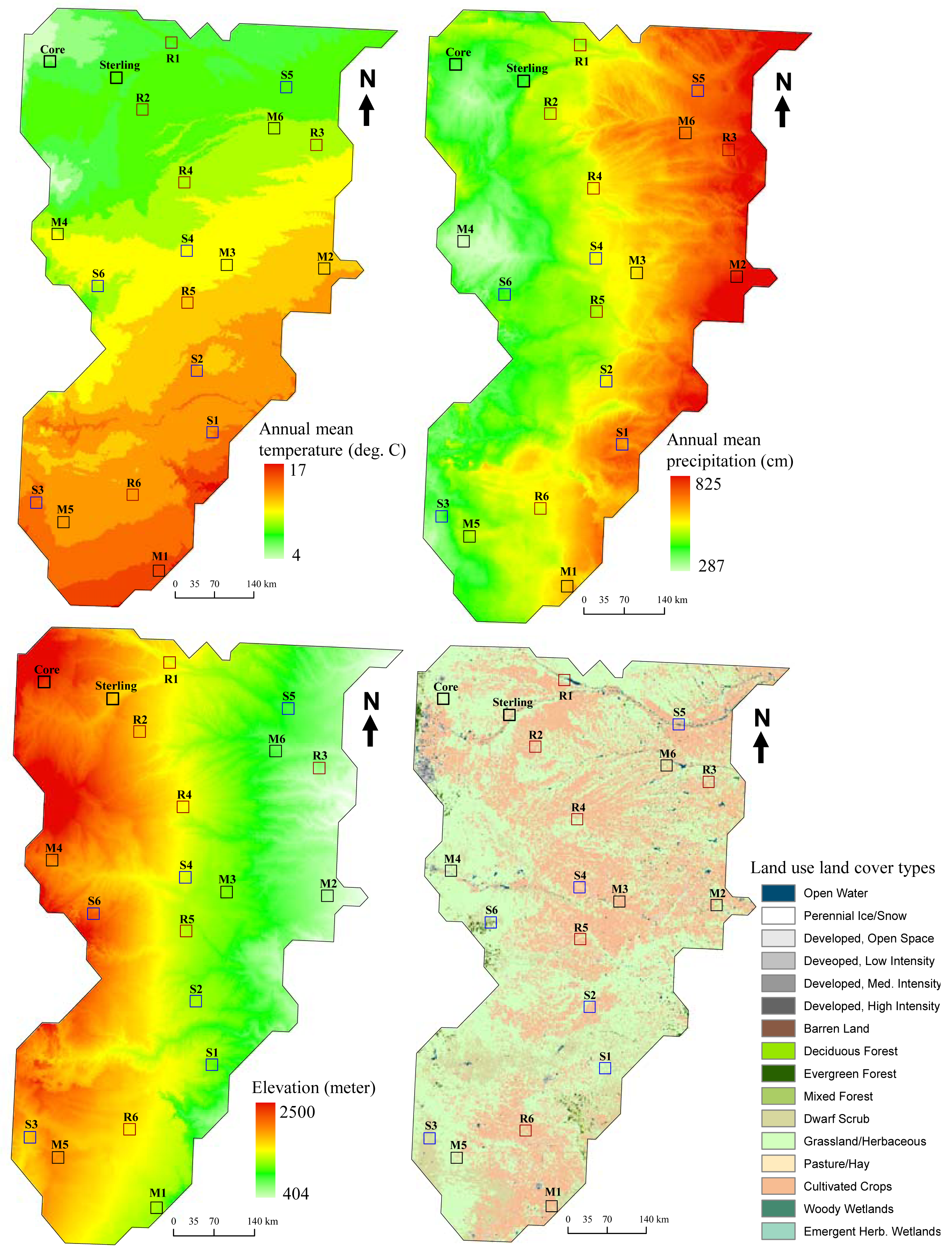
The predominant vegetation at the core site is C4-dominated native shortgrass steppe, and a variety of other communities in the domain (e.g., southern mixed grass and cool season species) are also present. The climate at the core site is characterized by low precipitation, periodic water deficits, and large interannual and interseasonal climatic fluctuations. Most (70%) of the annual precipitation is derived from the Gulf of Mexico and falls during the warm season between April and September. However, mean temperature and precipitation, elevation, and vegetation are highly variable across the domain (Figure 1). It is clear that additional ecological observatory sites will be needed to capture the major environmental gradients and heterogeneity across the domain.
2.2. Environmental Variables
Environmental factors used in this example included mean annual temperature and precipitation from Daymet climate dataset [16] (1980–1997), elevation [17], and land use land cover types [18]. These variables were chosen based on the strong east-west climatic and elevational gradients in this domain. All these layers were clipped to the extent of the Central Plains domain (1 km spatial resolution, Albers Equal Area projection).
2.3. Maxent Model
There are many species-environmental matching models. We used a relatively newer method which has consistently fared well in model comparison studies [3,6,7]. The maximum entropy model, Maxent, is a general purpose predictive model that relies on presence—only data [4,5]. Based on the principle of maximum entropy, Maxent integrates available information as constraints and obtains the least-biased inferences when insufficient information is available. This method estimates the probability distribution of a species by finding the probability distribution of maximum entropy, which is a probability that is closest to uniform [4]. Maxent produces a habitat suitability surface with probability values varying from 0 (least suitable or most dissimilar) to 1 (most suitable or most similar to presence cells). Maxent automatically calculates percent contribution of different environmental variables to the model. In our case, presence data reflected a NEON site, and was operationally defined as a 20 km × 20 km area that approximates the footprint of the NEON airborne observation platforms (AOP; 12). Each 1 km2 cell in the 400 km2 area was designated as a presence location, the model selected pseudo-absence cells (or background points) randomly from the remainder of the domain. The resulting probability of occurrence or habitat suitability model is comprised 1 km2 cells assigned a likelihood of similarity to the presence cells.
The initial models incorporated presence data from the NEON core site at the CPER and the North Sterling, Colorado relocatable site (first one, then the two sets of 400 presence cells). With the mean probability of occurrence output surface, we mapped areas in the domain that were the most dissimilar (probability of suitable habitat less than 0.1 × 10⁻⁶) to the environmental envelope captured by the NEON sites (probability of suitable habitat > 0.1). We randomly selected a new sample site—a hypothetical NEON relocatable site—from the frame of most dissimilar cells, buffered the site to account for environmental variability captured by the 400 km2 airborne observations, and ran the Maxent model with the three sites (three sets of 400 presence points). We repeated this process until we captured >75% of the cells in the domain.
Maxent (version 3.3.0) was used for the modeling and is freely available [4]. The validation of predictive model outputs from Maxent was accomplished by using the area under the receiver operating characteristic (ROC) curve or AUC; automatically calculated by Maxent (4) for each model step. At each step 10 replicates were run using 75% of the data for training the model and 25% data for validation, and average AUC was calculated.
We compared the efficacy of this Maxent Dissimilarity Sampling approach to two other commonly used sampling strategies. In both cases, we kept the CPER core site and North Sterling site and generated six new sites of the same size and shape as used in the Maxent approach described above (20 km × 20 km). We generated a stratified random design by adding six new sites stratified by temperature (high versus low), precipitation (high versus low), elevation (high versus low) and dominant vegetation (two classes, grassland and forest). We created a simple random sample design by randomly selecting six sites across the domain. We compared how each design captured the dominant environmental gradients of the domain with eight total sample sites.
3. Results and Discussion
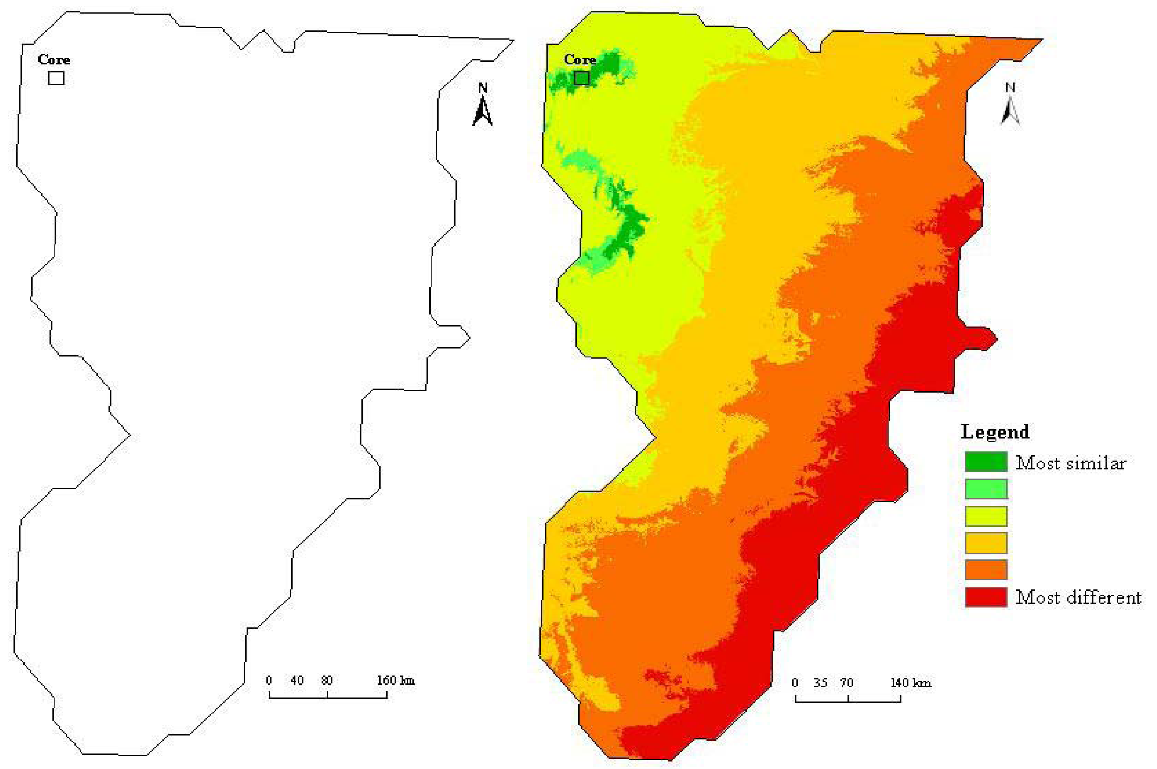
Maximum entropy modeling quickly identified similar and dissimilar habitats after the initial model run on the core site (Figure 2). Similar habitats, based on temperature, precipitation, elevation, and vegetation type were located in close proximity to the CPER site. The most dissimilar sites, according to the model, were located to the far southeast in the domain. A sampling design based solely on dissimilarity would have placed the second site in the most dissimilar region. However, to capture land use variations (intensive agriculture versus short grass steppe) and for logistical reasons (cost being a driving concern), the North Sterling site has been proposed as the first relocatable site (Figure 3b).
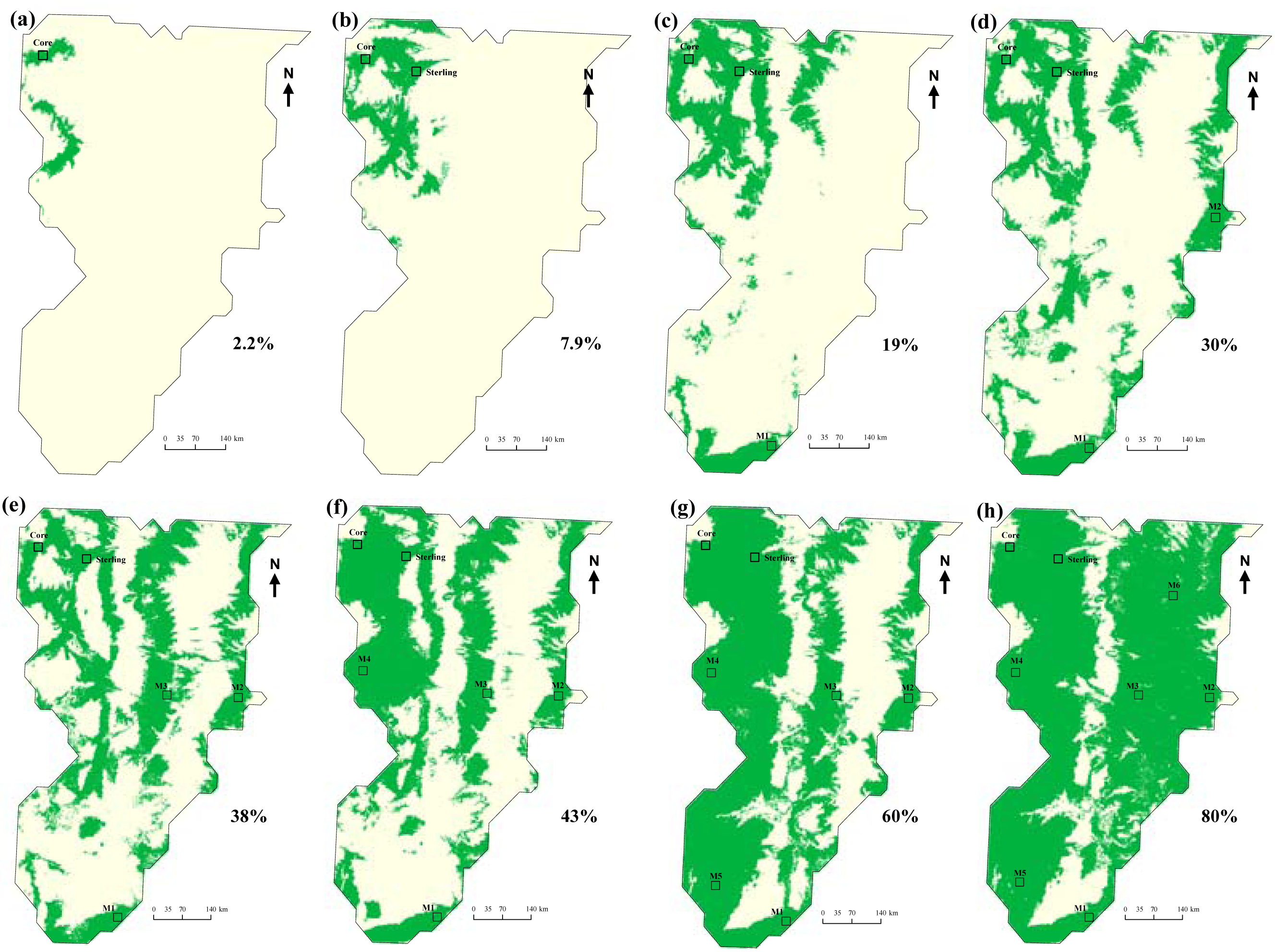
The question remained, where should the third, fourth, fifth, and so on, sites be located to adequately capture the heterogeneity of the domain? Locating the third site according to model-directed habitat dissimilarity in the southeast portion of the domain resulted in a model that captured about 19% of the domain in the environmental envelope of the sites (Figure 3c) as compared to just 2.2% (Figure 3a), and 7.9% (Figure 3b), after the first two runs.
The maximum entropy approach to selecting dissimilar sampling sites showed that after selecting six additional site locations following the two “fixed sites” at the Central Plains Experimental Range site and North Sterling, Colorado, that 80% of the domain's environmental envelop could be captured (Figure 3h). Elevation and precipitation differences across the domain contributed more significantly to the models compared to temperature and vegetation type (Table 1). After the final model, elevation and precipitation combined contributed 83.4% to the model.
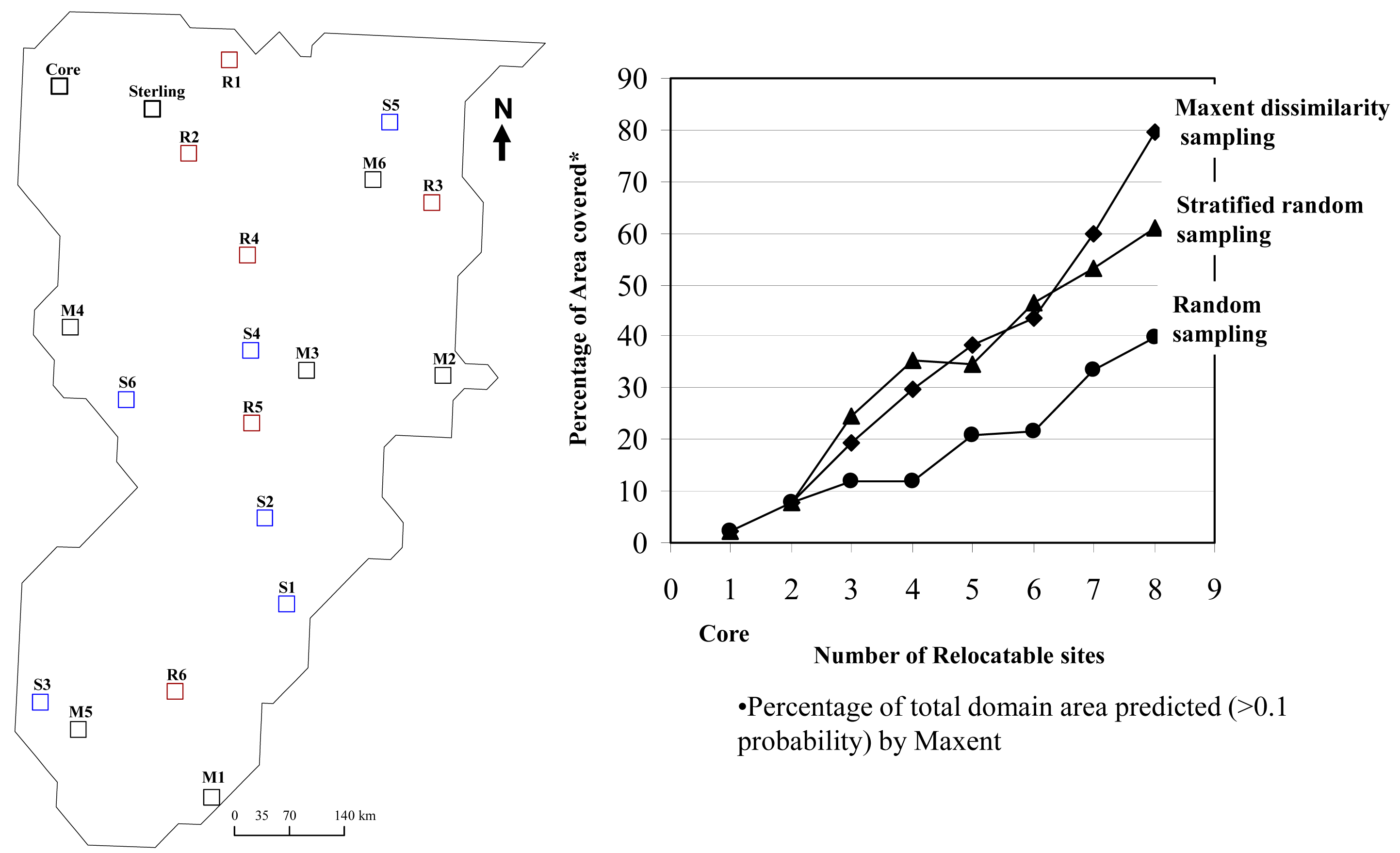
The percentage of the area covered (green areas in the successive models; Figure 3), tended to increase in a linear fashion as new sites were added (Figure 4). The final two sites filled in more of the gaps in environmental space, compared to the first two sites.
Keeping the core site and Sterling site set for each design, the stratified random design initially captured more of the environmental gradients of the domain by selecting sites in rare forested vegetation types (Figure 4). However, after six new sites were added, the Maxent Dissimilarity Sampling approach captured more of the total natural variation in the domain. Adding six randomly selected sites failed to capture as much of the dominant environmental gradients in the domain (Figure 4).
3.1. Discussion
There are many caveats associated with species-environmental matching models. All such models are affected by sample size, extent of the study area, the clustering of presence points, and the resolution and accuracy of predictive layers [4,5,19]. The clustering problem is especially relevant to this approach, where the presence points were forced to be clustered in a 20 km × 20 km area. This artificially inflates AUC values (Table 1), especially in the initial modeling stage. Likewise, the sample was spatially restricted ranging from just 400 to 3200 1 km2 cells, or just 0.09% to 0.71% of the domain. In addition, we placed new sites in the lowest probability of similarity (highest areas of dissimilarity; probability < 0.1 × 10⁻⁶) without comparing alternative sites at each stage.
A cost layer could be superimposed on the sampling scheme to compare the trade-offs in sample site selection. In this case study, dissimilar sites were far from the core site, primarily because it was selected in a distinct (higher elevation, low precipitation) area in the domain. The costs associated with capturing the environmental extremes in the domain cannot be easily avoided in this case. We also note that for most NEON domains, the design for relocatable sites emphasizes land-use contrasts. Capturing the environmental heterogeneity within a given domain is not the main driver for relocatable site selection [12].
3.2. General Utility of This Approach
The selection of potential sites for environmental monitoring is objective-driven [20]. However, designers commonly wish to extrapolate information in space and over time, to an entire region or area of interest. The maximum entropy modeling approach described above may have general application from landscape scales to continental scales. Additional climatic, topographic, phenological, and environmental factors can be easily included (e.g., [6,21]). However, in many cases, only a handful of factors may contribute heavily to model outcomes. In our test case, elevation and precipitation dominated the model.
The maximum entropy approach has many advantages over other approaches. It is a multivariate, non-parametric approach, handles non-linearities in the predictor variables well, and is largely unaffected by high cross-correlations and spatial autocorrelation among variables [4,5]. There is no guarantee that a small set of monitoring sites will effectively capture all the important changes the future may hold. It would become increasingly difficult to use a stratified sampling approach when more environmental strata are included. This is likely less of a problem when additional strata (layers) are added in the Maxent Dissimilarity Sampling approach. Thus, this probability based approach provides an unbiased method for selecting a small number of sites across many key environmental gradients.


| Model | Average validation AUC | Mean annual temperature (°C) | Mean annual precipitation (cm) | Elevation (m) | Land use land cover types |
|---|---|---|---|---|---|
| Core | 0.996 | 3.8 | 32.6 | 63.3 | 0.4 |
| Core + Sterling | 0.993 | 24.5 | 57.7 | 17.3 | 0.5 |
| Core + Sterling + 1 | 0.992 | 37.8 | 32.1 | 28.8 | 1.3 |
| Core + Sterling + 1 to 2 | 0.989 | 29.6 | 37.8 | 29.5 | 3.2 |
| Core + Sterling + 1 to 3 | 0.983 | 19.1 | 34.3 | 41.7 | 4.9 |
| Core + Sterling + 1 to 4 | 0.973 | 16.2 | 42.4 | 38.8 | 2.6 |
| Core + Sterling + 1 to 5 | 0.949 | 12.0 | 36.9 | 48.1 | 2.9 |
| Core + Sterling + 1 to 6 | 0.929 | 12.4 | 34.6 | 48.8 | 4.3 |
Acknowledgments
The U.S. Geological Survey, Fort Collins Science Center, and the Natural Resource Ecology Laboratory at Colorado State University provided logistical support. Funding for TJS was provided by the Invasive Species Program of the U.S. Geological Survey and USDA CSREES/NRI 2008-35615-04666. Funding for DTB and SK was provided by NEON Inc. Michael Keller, and Tracy Holcombe provided helpful reviews on an earlier version of the manuscript. Any use of trade, product, or firm names is for descriptive purposes only and does not imply endorsement by the U.S. Government. Two anonymous peer reviewers provided additional comments. To all we are grateful.
References
- Fortin, M.J.; Drapeau, P.; Legendre, P. Spatial auto-correlation and sampling design in plant ecology. Vegetatio 1989, 83, 209–222. [Google Scholar]
- Stohlgren, T.J. Measuring Plant Diversity, Lessons from the Field; Oxford University Press: New York NY, USA, 2007. [Google Scholar]
- Elith, J.; Graham, C.H.; Anderson, R.P.; Dudik, M.; Ferrier, S.; Guisan, A.; Hijmans, R.J.; Huettmann, F.; Leathwick, J.R.; Lehmann, A.; et al. Novel methods improve prediction of species' distribution from occurence data. Ecography 2006, 29, 129–151. [Google Scholar]
- Phillips, S.J.; Anderson, R.P.; Schapire, R.E. Maximum entropy modeling of species geographic distributions. Ecol. Model. 2006, 190, 231–259. [Google Scholar]
- Phillips, S.J.; Dudik, M.; Schapire, R.E. A maximum entropy approach to species distribution modeling. Proceedings of the 21st International Conference on Machine Learning, Banff Alberta, Canada, 4–8 July 2004; Brodley, C.E., Ed.; Association for Computing Machinery: New York, NY, USA, 2004. [Google Scholar]
- Kumar, S.; Spaulding, S.A.; Stohlgren, T.J.; Hermann, K.A.; Schmidt, T.S.; Bahls, L.L. Predicting habitat distribution for freshwater diatom Didymosphernia geminata in the continental United States. Front. Ecol. Environ. 2009, 7, 415–420. [Google Scholar]
- Li, M.Y.; Ju, Y.W.; Kumar, S.; Stohlgren, T.J. Modeling potential habitats for alien species Dreissena polymorpha (Zebra mussel) in the Continental USA. Acta Ecol. Sin. 2008, 28, 4253–4258. [Google Scholar]
- Evangelista, P.H.; Kumar, S.; Stohlgren, T.J.; Jarnevich, C.S.; Crall, A.W.; Norman, J.B., III; Barnett, D.T. Modeling invasion for a habitat generalist and a specialist plant species. Diversity Distr. 2008, 14, 808–817. [Google Scholar]
- Jarnevich, C.S.; Stohlgren, T.J. Near term climate projections for invasive species distributions. Biol. Invasions. 2009, 11, 1373–1379. [Google Scholar]
- Pawar, S.; Koo, M.S.; Kelley, C.; Ahmed, M.F.; Chaudhuri, S.; Sarkar, S. Conservation assessment and prioritization of areas in Northeast India: Priorities for amphibians and reptiles. Bio. Conservat. 2007, 136, 346–361. [Google Scholar]
- Fuller, T.; Morton, D.P.; Sarkar, S. Incorporating uncertainty about species' potential distributions under climate change into the selection of conservation areas with a case study from the Arctic Coastal Plain of Alaska. Biol. Conservat. 2008, 141, 1547–1559. [Google Scholar]
- Keller, M.; Schimel, D.S.; Hargrove, W.W.; Hoffman, F.M. A continental strategy for the National Ecological Observatory Network. Front. Ecol. Environ. 2008, 6, 282–284. [Google Scholar]
- Hargrove, W.W.; Hoffman, F.M. Using multivariate clustering to characterize ecoregion borders. Comput. Sci. Eng. 1999, 1, 18–25. [Google Scholar]
- Hargrove, W.W.; Hoffman, F.M. The potential of multivariate quantitative methods for delineation and visualization of ecoregions. Environ. Manag. 2004, 34, S39–S60. [Google Scholar]
- National Ecological Observatory Network Home Page: Boulder, CO, USA, 2011. Available online: http://www.neoninc.org/ (accessed on 24 May 2011).
- Daily Surface Weather and Climatalogical Summaries Home Page: Oak Ridge, TN, USA, 2011. Available online: http://www.daymet.org/ (accessed on 24 May 2011).
- USGS Hydro 1K. U.S. Geological Survey: Reston, VA, USA, 2010. Available online: http://edc.usgs.gov/products/elevation/gtopo30/hydro/index.html (accessed on 24 May 2011).
- Vogelmann, J.E.; Howard, S.M.; Yang, L.M.; Larson, C.R.; Wylie, B.K.; van Driel, N. Completion of the 1990s National Land Cover Dataset for the conterminous United States from Landsat Thematic Mapper data and ancillary data sources. Photogramm. Eng. Rem. Sens. 2001, 67, 650–662. [Google Scholar]
- Pearson, R.G.; Raxworthy, C.J.; Nakamura, M.; Peterson, A.T. Predicting species distributions from small numbers of occurrence records: A test case using cryptic geckos in Madagascar. J. Biogeogr. 2007, 34, 102–117. [Google Scholar]
- Rose, K.A.; Smith, E.P. Experimental design: The neglected aspect of environmental monitoring. Environ. Manag. 1992, 16, 691–700. [Google Scholar]
- Morisette, J.T.; Richardson, A.D.; Knapp, A.K.; Fisher, J.I.; Graham, E.A.; Abatzoglou, J.; Wilson, B.E.; Breshears, D.D.; Henebry, G.M.; Hanes, J.M.; Liang, L. Tracking the rhythm of the seasons in the face of global change: Phenological research in the 21st century. Front. Ecol. Environ. 2009, 7, 253–260. [Google Scholar]
© 2011 by the authors; licensee MDPI, Basel, Switzerland. This article is an open access article distributed under the terms and conditions of the Creative Commons Attribution license (http://creativecommons.org/licenses/by/3.0/).
Share and Cite
Stohlgren, T.J.; Kumar, S.; Barnett, D.T.; Evangelista, P.H. Using Maximum Entropy Modeling for Optimal Selection of Sampling Sites for Monitoring Networks. Diversity 2011, 3, 252-261. https://doi.org/10.3390/d3020252
Stohlgren TJ, Kumar S, Barnett DT, Evangelista PH. Using Maximum Entropy Modeling for Optimal Selection of Sampling Sites for Monitoring Networks. Diversity. 2011; 3(2):252-261. https://doi.org/10.3390/d3020252
Chicago/Turabian StyleStohlgren, Thomas J., Sunil Kumar, David T. Barnett, and Paul H. Evangelista. 2011. "Using Maximum Entropy Modeling for Optimal Selection of Sampling Sites for Monitoring Networks" Diversity 3, no. 2: 252-261. https://doi.org/10.3390/d3020252