Prognosis of the Remaining Useful Life of Bearings in a Wind Turbine Gearbox

Abstract

Predicting the remaining useful life (RUL) of critical subassemblies can provide an advanced maintenance strategy for wind turbines installed in remote regions. This paper proposes a novel prognostic approach to predict the RUL of bearings in a wind turbine gearbox. An artificial neural network (NN) is used to train data-driven models and to predict short-term tendencies of feature series. By combining the predicted and training features, a polynomial curve reflecting the long-term degradation process of bearings is fitted. Through solving the intersection between the fitted curve and the pre-defined threshold, the RUL can be deduced. The presented approach is validated by an operating wind turbine with a faulty bearing in the gearbox.

1. Introduction

More and more attention is being given to the maintenance of wind turbines installed in remote regions [1,2,3]. This attention is due to the difficulty of transporting and hoisting wind turbine parts. Conventional methods of replacing failed subassemblies in wind turbines cause long downtimes. Remaining useful life (RUL) prognostics enable early detection of faultiness and estimation of the failure time of subassemblies in wind turbines, further helping operators to schedule a reasonable maintenance plan and save operational costs.

Plenty of approaches have been developed to monitor the health conditions of wind turbines. Yang et al. [4] utilized electrical signals to discover windings faults in wind turbine generators. Teng et al. [5] adopted offline vibration analysis to detect multiple faults in wind turbine gearboxes. Kusiak and Verma [6] analyzed the temperature signals from the supervisory control and data acquisition system to predict bearing faults in generators. Dupuis [7] used oil debris to monitor wind turbine gearboxes and provide an early indication of internal damage to bearings and gears. Strain gauges and acoustic emission were used for fault detection in blades, bearings and shafts [8]. Condition monitoring systems are good at finding defects existing in machinery subassemblies, but they seldom allow the estimation of the RUL of faulty parts in wind turbines.

Data-driven based approaches are widely applied to estimate the RUL of rotating machineries. Tian et al. [9,10] proposed a neural network (NN) model to predict RUL of pump bearings using historical failure and suspension data. Ali et al. [11] adopted a simplified fuzzy-adaptive resonance theory map NN with Weibull distribution to predict the RUL of bearings. Zio et al. [12] applied particle filtering to estimate the RUL of a mechanical component subject to fatigue crack growth. Chen et al. [13] combined adaptive neuro-fuzzy inference systems and high-order particle filtering to forecast the RUL of planetary gear plates in a helicopter. Nonlinear feature reduction [14] and exponential regression [15] are integrated with a support vector machine to predict the residual useful life of a bearing. Boskoski et al. [16] used Renyi entropy based features and Gaussian process models to anticipate the RUL of bearings. Sikorska et al. [17] summarized the modelling approaches for predicting the RUL of engineering assets in a real industrial environment.

The majority of the above research focused on predicting the RUL of bearings through training life cycle models. However, this approach is not suitable for the RUL estimation of wind turbines for several reasons: (i) multiple gears and bearings in the gearbox make it difficult to acquire the same failure datasets; e.g., the failure parts may be diverse in the same types of wind turbines from the same wind farm; (ii) varying operational conditions disturb the degradation process of critical parts [18]; and (iii) the degradation tendencies of training dataset do not always accord with the testing dataset, even for the same type of parts [19].

In this paper, a novel RUL prognostic approach without life cycle training models is proposed to predict the RUL of bearings in wind turbine gearbox. The remainder of the paper is organized as follows: the structure of the drive train of wind turbines is presented, and the transmission ratios of different stages in a gearbox are calculated in Section 2. Section 3 proposes the NN-based prediction method of short-term feature tendencies and the estimation procedure of the RUL. In Section 4, the proposed approach is validated by studying an operating wind turbine with a faulty bearing in the gearbox. Conclusions are drawn in Section 5.

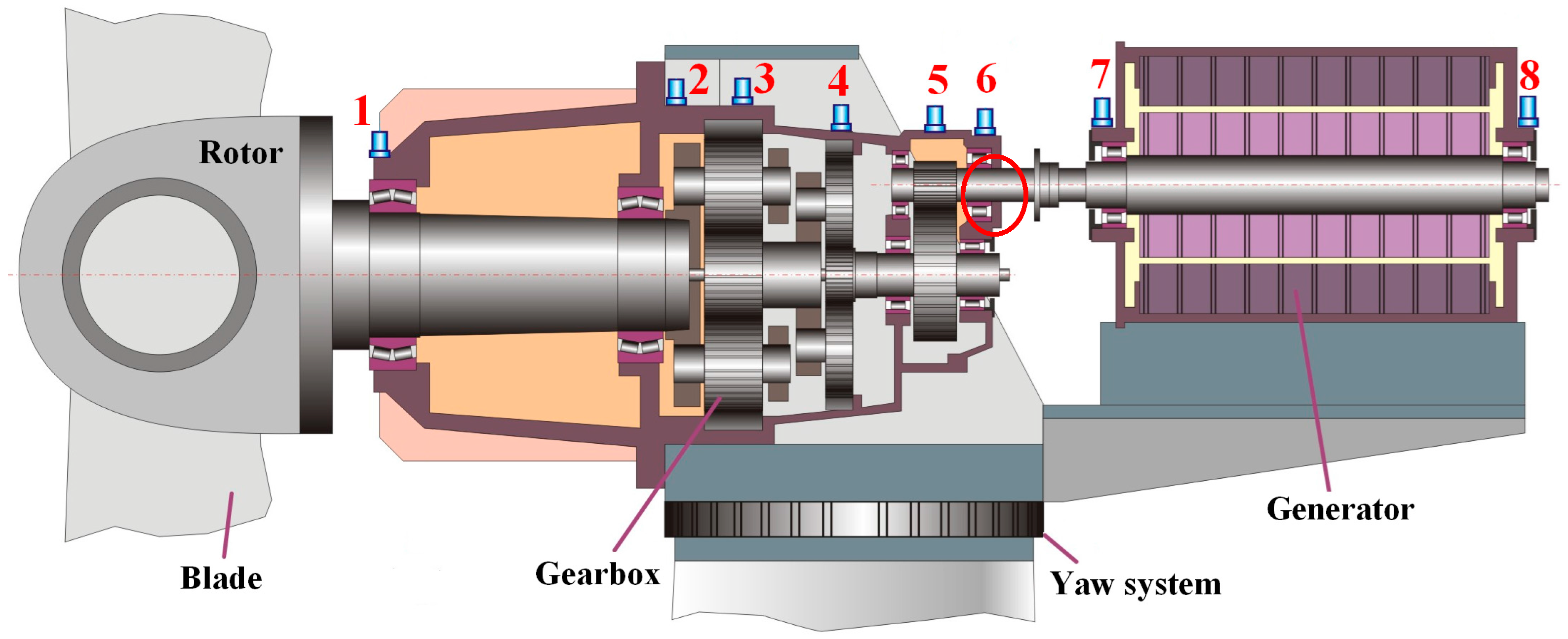
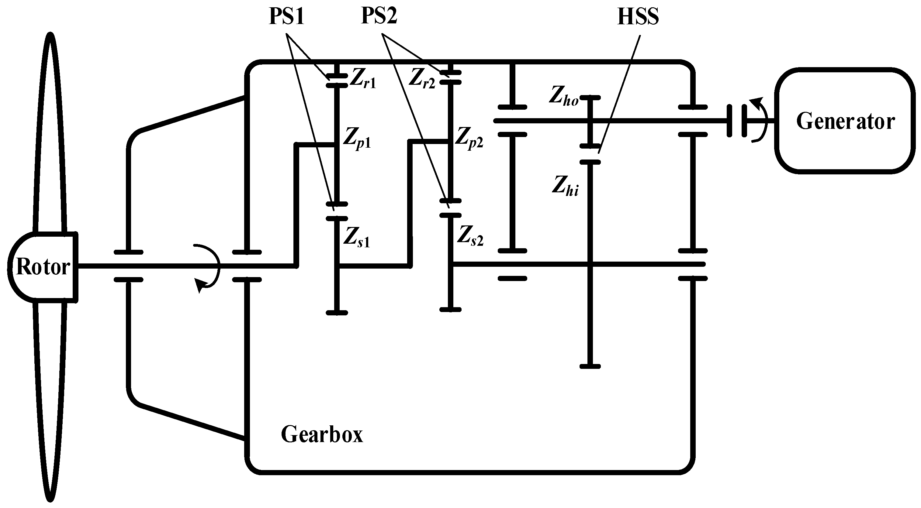
2. Wind Turbine Drive Train

The drive train of mainstream wind turbines shown in Figure 1 consists of a rotor, gearbox and generator. The rotor connecting with three blades converts wind energy into low speed mechanical energy which in turn is speeded up by the gearbox. The drive train involves multiple critical parts e.g., gears, bearings and shafts. Eight acceleration transducers are installed on the surface of the drive train to monitor its health condition. Each transducer is responsible for the adjacent parts.

The gearbox in this paper is composed of two planetary stages (PS1, PS2), and a high speed stage (HSS). In the schematic diagram of the gearbox shown in Figure 2, Z_s1, Z_p1 and Z_r1 denote the sun gear, planetary gear, and ring gear, respectively. They make up the first planetary stage (PS1). Similarly, Z_s2, Z_p2 and Z_r2 compose the second planetary stage (PS2). Big gear Z_hi and gear Z_ho on the high speed shaft mesh and form the HSS.

The transmission ratio of the planetary stage is computed from Equation (1):

$$r_{\mathrm{PS}}=1+\frac{Z_r}{Z_s}$$

(1)

where Z_r is the number of teeth of ring gear in planetary stage, Z_s is the number of teeth of sun gear in planetary stage. The transmission ratio r_PS1 of the PS1 and r_PS2 of the PS2 can be obtained according to Equation (1).

The transmission ratio of HSS is computed according to Equation (2):

$$r_{\mathrm{HSS}}=\frac{Z_{hi}}{Z_{ho}}$$

(2)

where Z_hi is the number of teeth of the big gear in HSS, Z_ho is the number of teeth of the gear on the high speed shaft. The total transmission ratio of gearbox is expressed in Equation (3):

$$r=r_{\mathrm{PS1}}\cdot r_{\mathrm{PS2}}\cdot r_{\mathrm{HSS}}$$

(3)

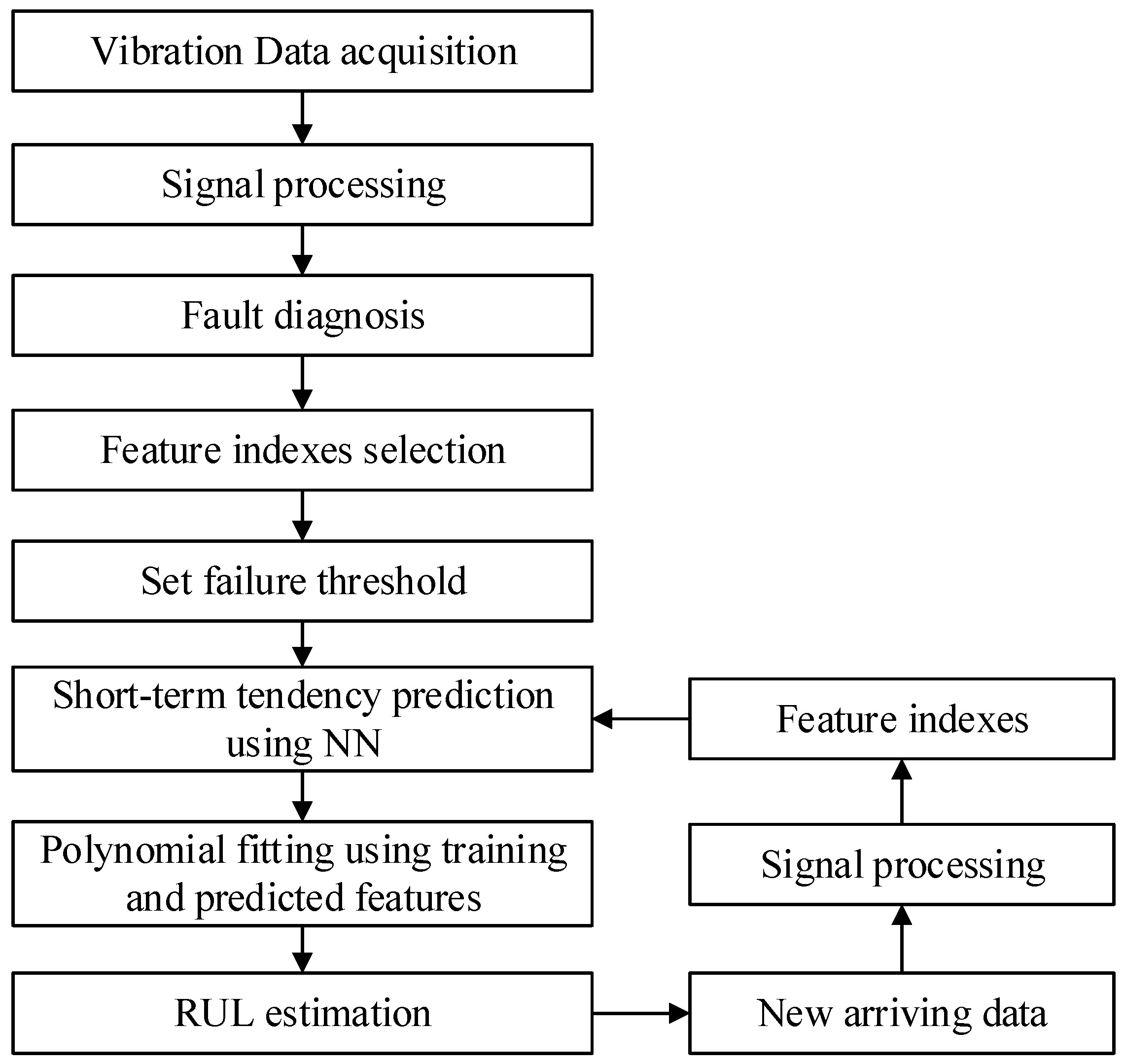
3. RUL Estimation of Bearings in Wind Turbine Gearbox

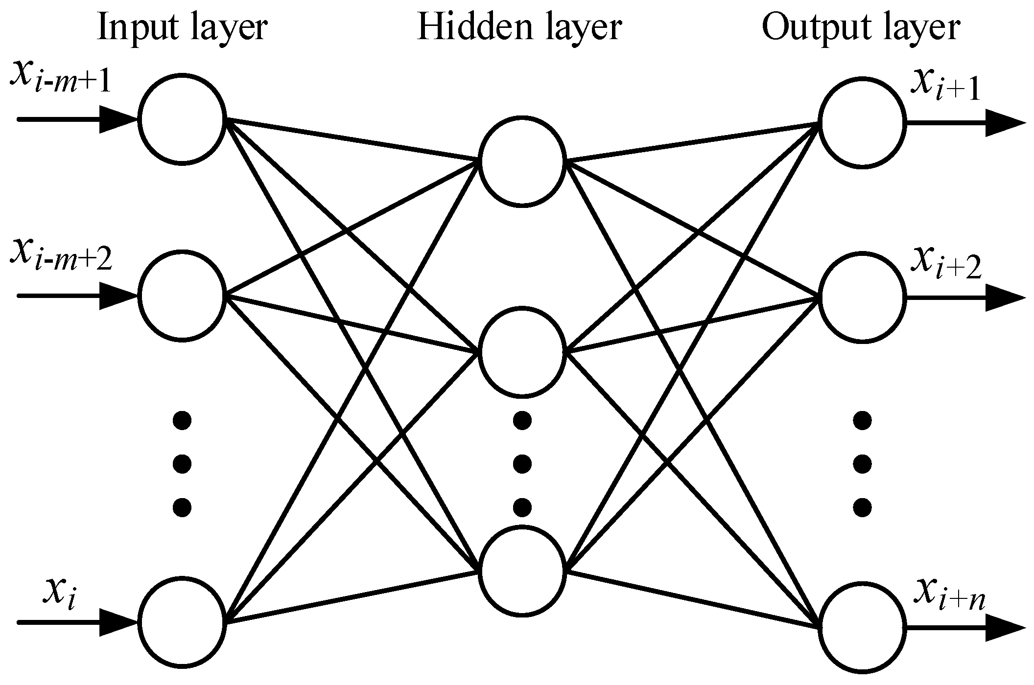
3.1. Neural Network for Short-Term Tendency Prediction

A NN [20] is a powerful tool that can construct arbitrary nonlinear relationships between input and output series. It is widely used in fault prognostics, e.g., RUL estimation of bearings [9,10,11] and tool wear recognition [21]. Here, a NN is adopted to train our model and predict the short-term tendency of feature series. Given the feature series $\mathit{x}=(x_1,x_2,\cdots ,x_L)$ denoting the degradation process of critical parts in wind turbine gearbox, the short-term prediction needs to use m historical features to calculate n future features, which is shown in Figure 3.

To guarantee a robust prognostic result, a scrolling prediction method is utilized. Assuming t = i + 1 (1 < i< L − 1) is the starting time of short-term prediction, m + n − 1 features before i + 1 are used to construct the input series shown in Equation (4):

$${\mathit{x}}_{in}=\left[\begin{array}{cccc}{x}_{i-n-m+2}& x_{i-n-m+3}& \cdots & x_{i-m+1}\\ x_{i-n-m+3}& x_{i-n-m+4}& \cdots & x_{i-m+2}\\ ⋮& ⋮& \cdots & ⋮\\ x_{i-n+1}& x_{i-n+2}& \cdots & x_i\end{array}\right]$$

(4)

Each column in Equation (4) is input into the trained NN model to obtain predicted features, which are described as Equation (5):

$${\widehat{\mathit{x}}}_{out}=\left[\begin{array}{cccc}{\widehat{x}}_{i-n+2}& {\widehat{x}}_{i-n+3}& \cdots & {\widehat{x}}_{i+1}\\ {\widehat{x}}_{i-n+3}& {\widehat{x}}_{i-n+4}& \cdots & {\widehat{x}}_{i+2}\\ ⋮& ⋮& \cdots & ⋮\\ {\widehat{x}}_{i+1}& {\widehat{x}}_{i+2}& \cdots & {\widehat{x}}_{i+n}\end{array}\right]$$

(5)

The mean of the back-diagonal elements in Equation (5) is regarded as the predicted feature ${\widehat{x}}_{i+1}$, then the input matrix is updated as Equation (6):

$${\mathit{x}}_{in}=\left[\begin{array}{cccc}{x}_{i-n-m+3}& x_{i-n-m+4}& \cdots & x_{i-m+2}\\ x_{i-n-m+4}& x_{i-n-m+5}& \cdots & x_{i-m+3}\\ ⋮& ⋮& \cdots & ⋮\\ x_{i-n+2}& x_{i-n+3}& \cdots & {\widehat{x}}_{i+1}\end{array}\right]$$

(6)

The new output series are expressed in Equation (7):

$${\widehat{\mathit{x}}}_{out}=\left[\begin{array}{cccc}{\widehat{x}}_{i-n+3}& {\widehat{x}}_{i-n+4}& \cdots & {\widehat{x}}_{i+2}\\ {\widehat{x}}_{i-n+4}& {\widehat{x}}_{i-n+5}& \cdots & {\widehat{x}}_{i+3}\\ ⋮& ⋮& \cdots & ⋮\\ {\widehat{x}}_{i+2}& {\widehat{x}}_{i+3}& \cdots & {\widehat{x}}_{i+n+1}\end{array}\right]$$

(7)

Similarly, the mean of the back-diagonal elements in Equation (7) is regarded as the predicted feature ${\widehat{x}}_{i+2}$. By this analogy, the predicted series are obtained as $({\widehat{x}}_{i+1},{\widehat{x}}_{i+2},\cdots ,{\widehat{x}}_{i+n+1})$.

The principle of selecting m and n is: within m time series, the tendency of fault feature can be reflected clearly, and m should be larger than n to guarantee reliable prediction results.

3.2. Procedure of Remaining Useful Life Estimation of Bearings

The prognostic procedure for determining the RUL is shown in Figure 4. First, the acquired vibration data is analyzed using advanced signal processing methods. Fault frequencies are calculated based on the structure of the wind turbine gearbox. Then, the potential fault is detected by comparing the analysis result of signal processing and fault frequencies. Next, the time of early fault detection is considered as the starting time of the RUL prognostic. The feature indexes reflecting the degradation tendencies of faulty parts are calculated and selected as prognostic objects. Meanwhile, the threshold of each feature index is set according to statistical analysis or existing criteria. Next, the short-term tendency of selected feature index is predicted using the NN described in the section above. A polynomial curve indicating long-term tendency of feature index is fitted on the basis of the training and predicted features, and the type of fitted curve is determined by observing the shape of the historical and short-term predicted features. Finally, the RUL is estimated through calculating the intersection of the fitted curve and pre-defined threshold.

When new vibration data become available, the corresponding feature indexes are supplemented into the former training features and used to estimate the RUL at current time. The prognostic process is implemented repeatedly until the faulty part fails.

Given the fitted curve f(t), the RUL of current time is estimated as Equation (8):

$$\mathrm{RUL}=f^{-1}(v_T)-t_c$$

(8)

where t_c is the current time, and $f^{-1}(v_T)$ is the estimated failure time under the fitted tendency curve f(t) and threshold v_T.

In industrial applications, affected by varying amplitude loads and background noise, individual features may fluctuate, which leads to an incorrect prognostic result, so multiple features need to be selected to calculate the weighted RUL expressed in Equation (9) to improve the stability of prognostic results:

$$\mathrm{RUL}={\displaystyle \sum _{k=1}^K{\mathrm{RUL}}_k\cdot w_k}$$

(9)

where RUL_k is the estimated RUL using an individual feature, K is the number of features, and w_k is the weight of the kth feature, ${\displaystyle {\sum }_{k=1}^K{w}_k=1}$.

4. Case Study

4.1. Testing Conditions

The rated power of the tested wind turbine is 1.5 MW. The total transmission ratio of the gearbox is 105. The number of teeth of the multi-stage gears in the wind turbine gearbox are shown in

Table 1. The numbers of teeth of multiple gears in wind turbine gearbox.

Zp1	Zs1	Zr1	Zp2	Zs2	Zr2	Zhi	Zho
40	23	104	37	27	102	92	23

.

On the basis of Equations (1)–(3) and Figure 2, the shaft rotational frequency and gear meshing frequency are shown in

Table 2. Shaft rotational frequencies and gear meshing frequencies.

fa1 (Hz)	fs1 = fa2 (Hz)	fs2 (Hz)	fh (Hz)	fPS1 (Hz)	fPS2 (Hz)	fHSS (Hz)
0.293	1.62	7.75	31.0	30.5	165.4	713

, where f_a1 is the rotational frequency of planet carrier in PS1, f_s1 = f_a1 × r_PS1 is the rotational frequency of sun gear in PS1, also the rotational frequency of planet carrier in PS2, and f_s2 = f_s1 × r_PS2 is the rotational frequency of sun gear in PS2, also the rotational frequency of big gear in HSS, f_h = f_s2 × r_HSS is the rotational frequency of high speed shaft. f_PS1 = f_a1 × Z_s1, f_PS2 = f_s1 × Z_s2 and f_HSS = f_s2 × Z_hi are the mesh frequencies of PS1, PS2 and HSS.

The health condition of the drive train is monitored by eight acceleration transducers installed as shown in Figure 1. Vibration data of 204.75 days are collected, which covers a complete life cycle process of a bearing in the gearbox. The faulty bearing is in the high speed shaft near the generator and its feature frequency is shown in

Table 3. Feature frequencies of bearings in the high speed shaft close to the generator.

Parts in the Bearing	Ratio to fr	Feature Frequency (Hz)
Cage fault	0.401	12.43
Rolling element fault	2.43	75.3
Outer race fault	5.21	161.5
Inner race fault	7.79	241.7

.

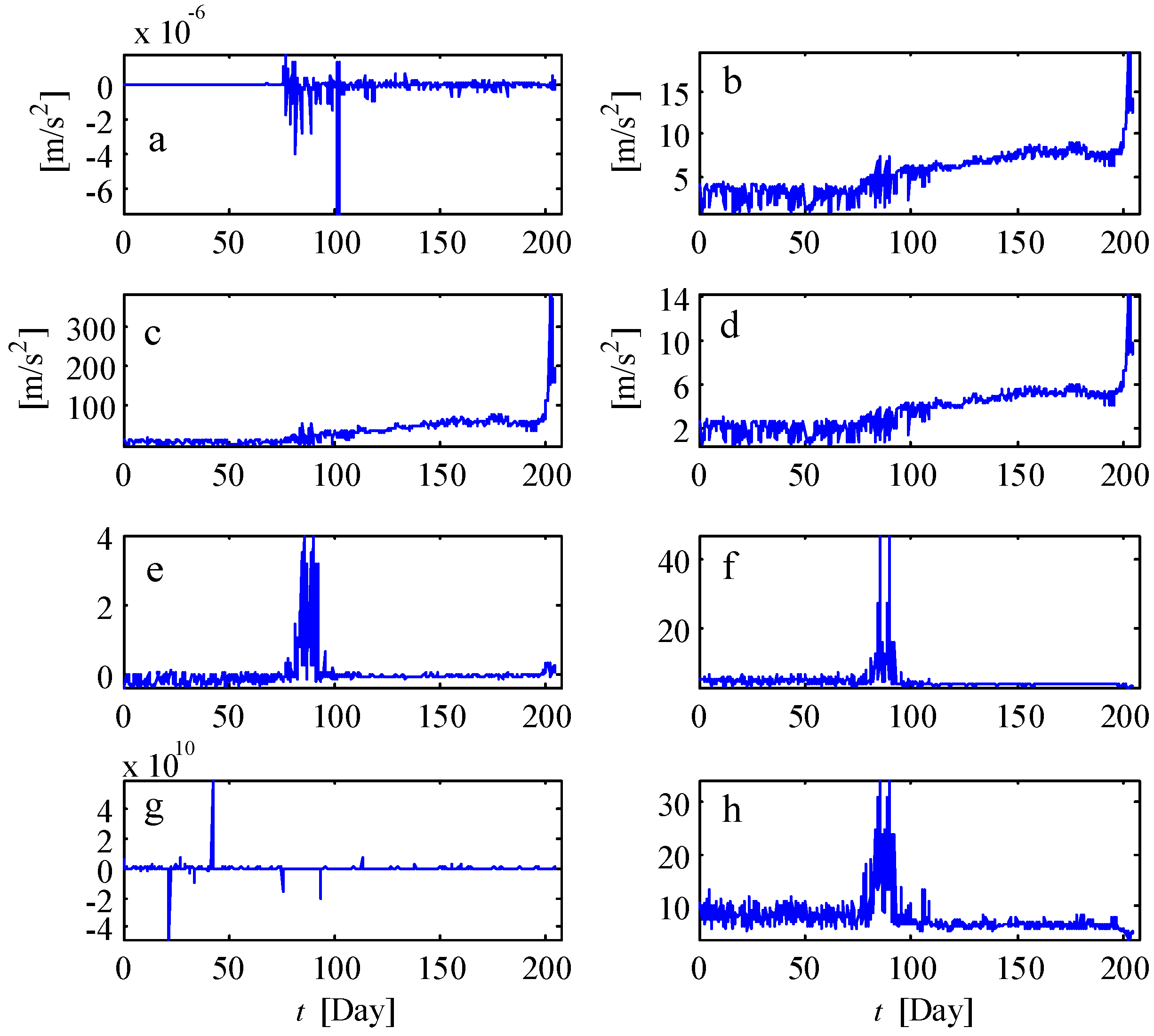
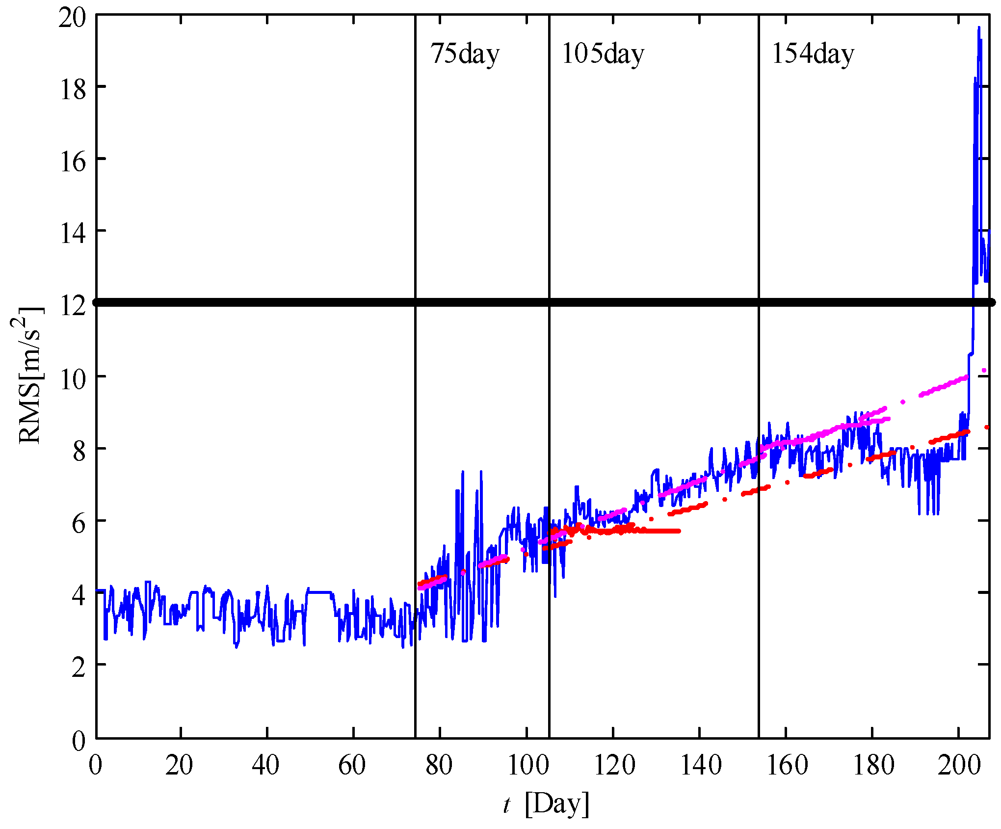
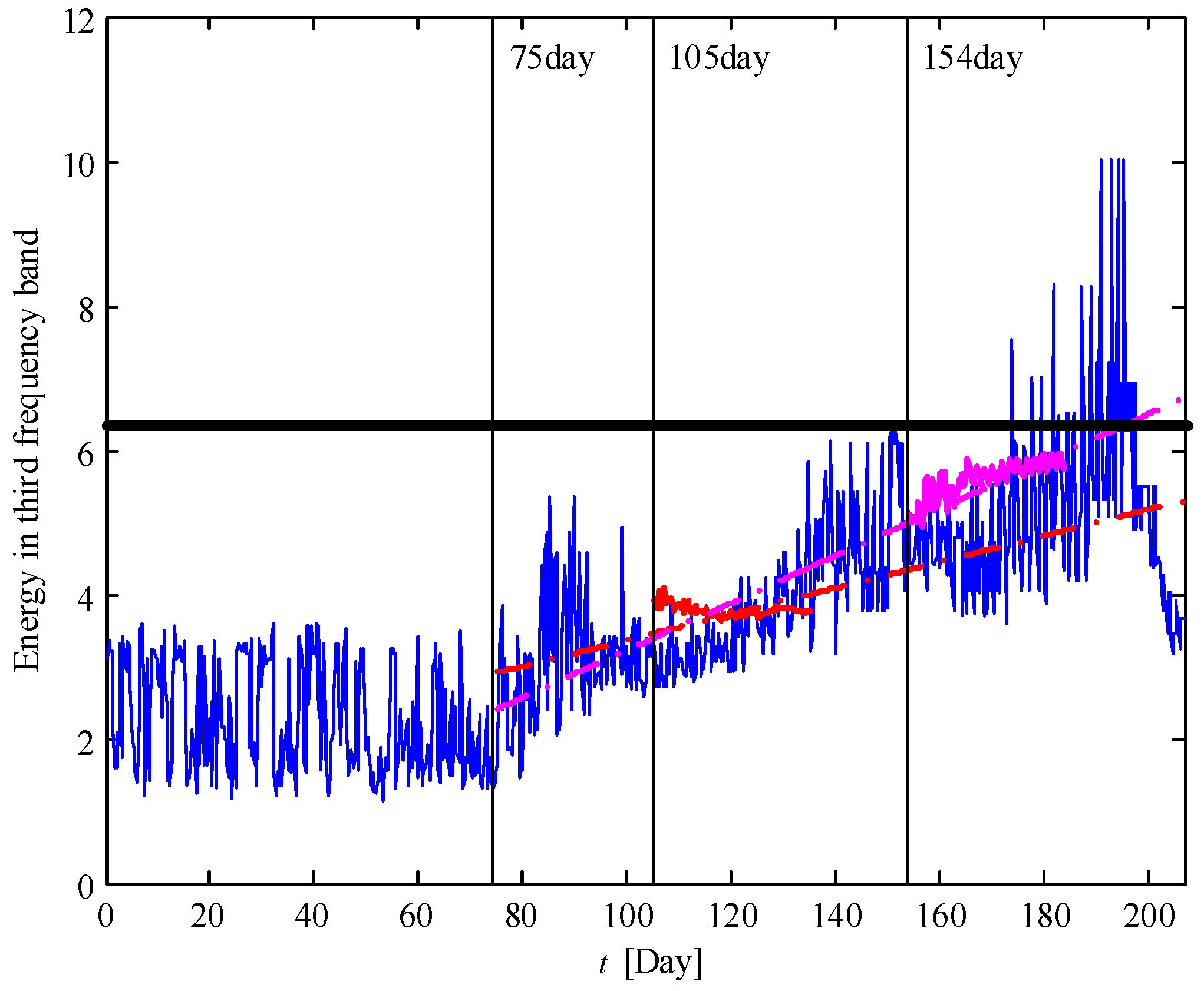
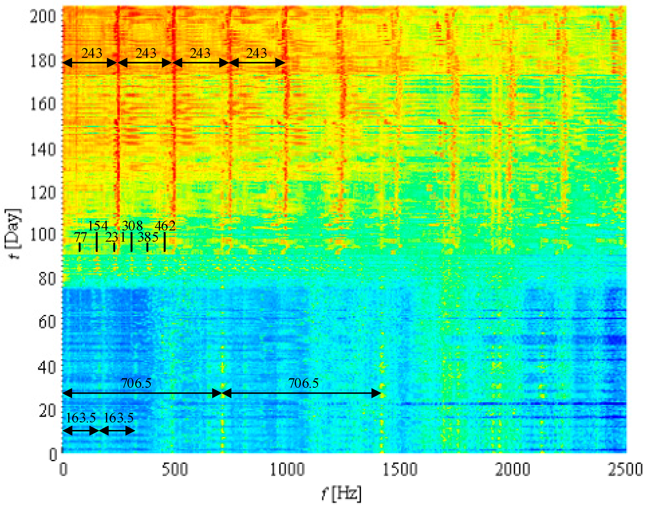
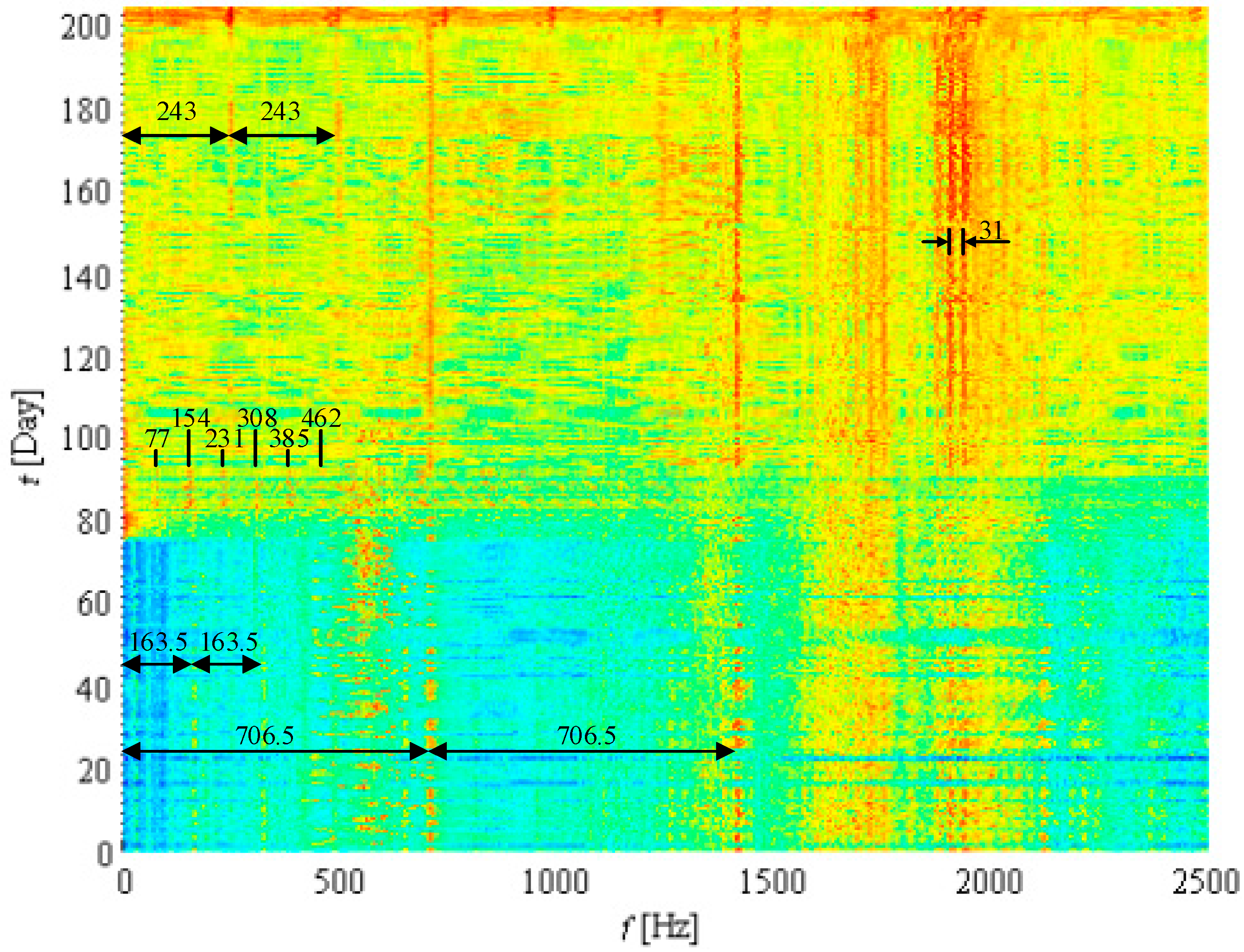
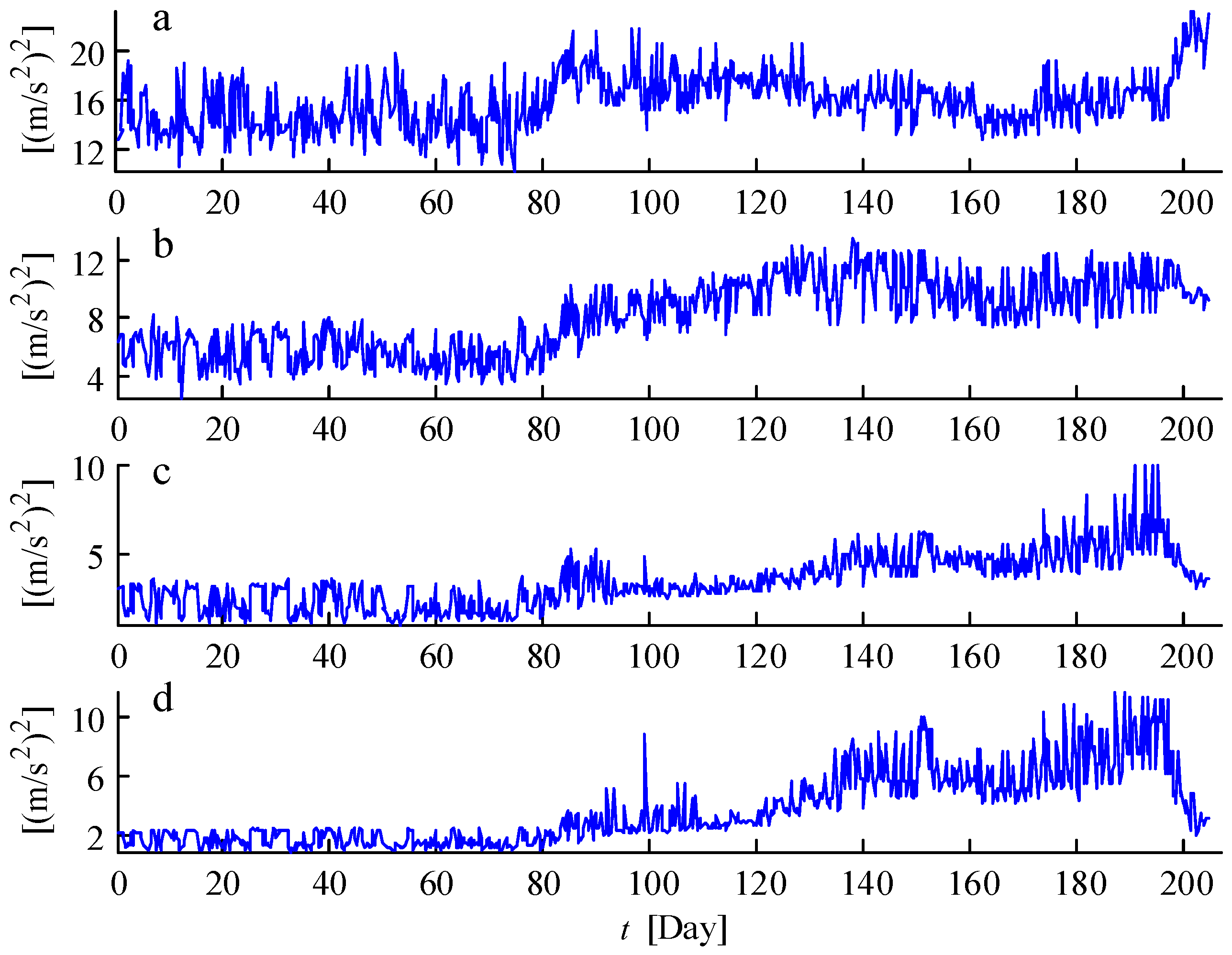
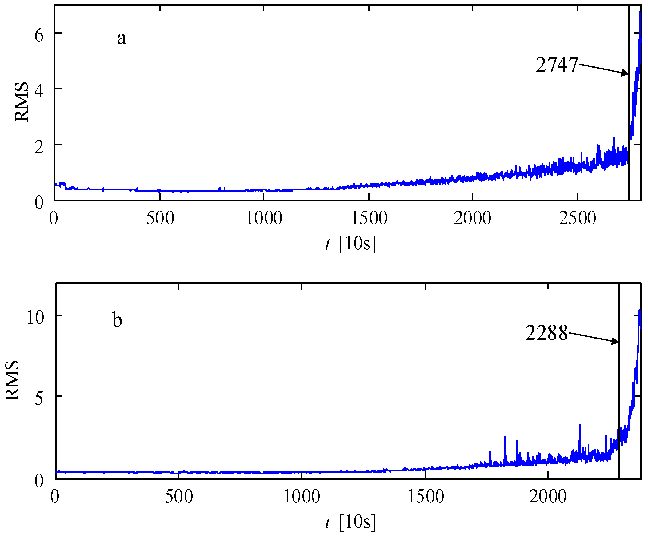
4.2. Fault Diagnosis for the Wind Turbine Gearbox

The vibration signals from the online monitoring system are sifted every six hours when the wind turbine is operating under the rated speed. Each sifted signal has a span of two seconds. The sampling frequency is 16,384 Hz. 819 groups of vibration signals of transducers 5 and 6 are shown in Figure 5, where the amplitudes enlarge at group 300 (the 75th day) and increase gradually until the end. The enlargement of amplitude from group 300 may indicate a fault in the wind turbine gearbox, and the increasing trend denotes the development process of this fault.

All the tested vibration signals are transformed into the frequency domain. The waterfalls of transducer 5 and 6 are shown in Figure 6 and Figure 7. From the first to the 300th group, the waterfall is dominated by 163.5 Hz and 706.5 Hz denoting the mesh frequencies of the second planetary stage and HSS in Table 2. This is a normal phenomenon since it accords with the dynamic principle that higher rotational speed generates more intensive vibration energy.

From the 301th (the 75.25th day) to the 380th (the 95th day) group, there are multi-harmonic frequencies of 77 Hz corresponding to the feature frequency of rolling element in Table 3, which reflects a fault arising on rolling balls of the bearing in the high speed shaft close to the generator. From the 381th (the 95.25th day) group to the end in Figure 6, another frequency 243 Hz and its harmonics become evident, which indicate a fault on the inner race of the bearing. The same frequency also emerges in Figure 7 from the 600th (the 150th day) group to the end.

The frequencies from the 75.25th day in Figure 6 and Figure 7 demonstrate faults starting to occur on the bearing in the high speed shaft of the wind turbine gearbox. This time is recognized as the initial time of estimating the RUL. The faulty bearing in the high speed shaft near the generator, circled in Figure 1, is one of the most fragile parts in the drive train of wind turbine due to the possible misalignment of the connection with the generator.

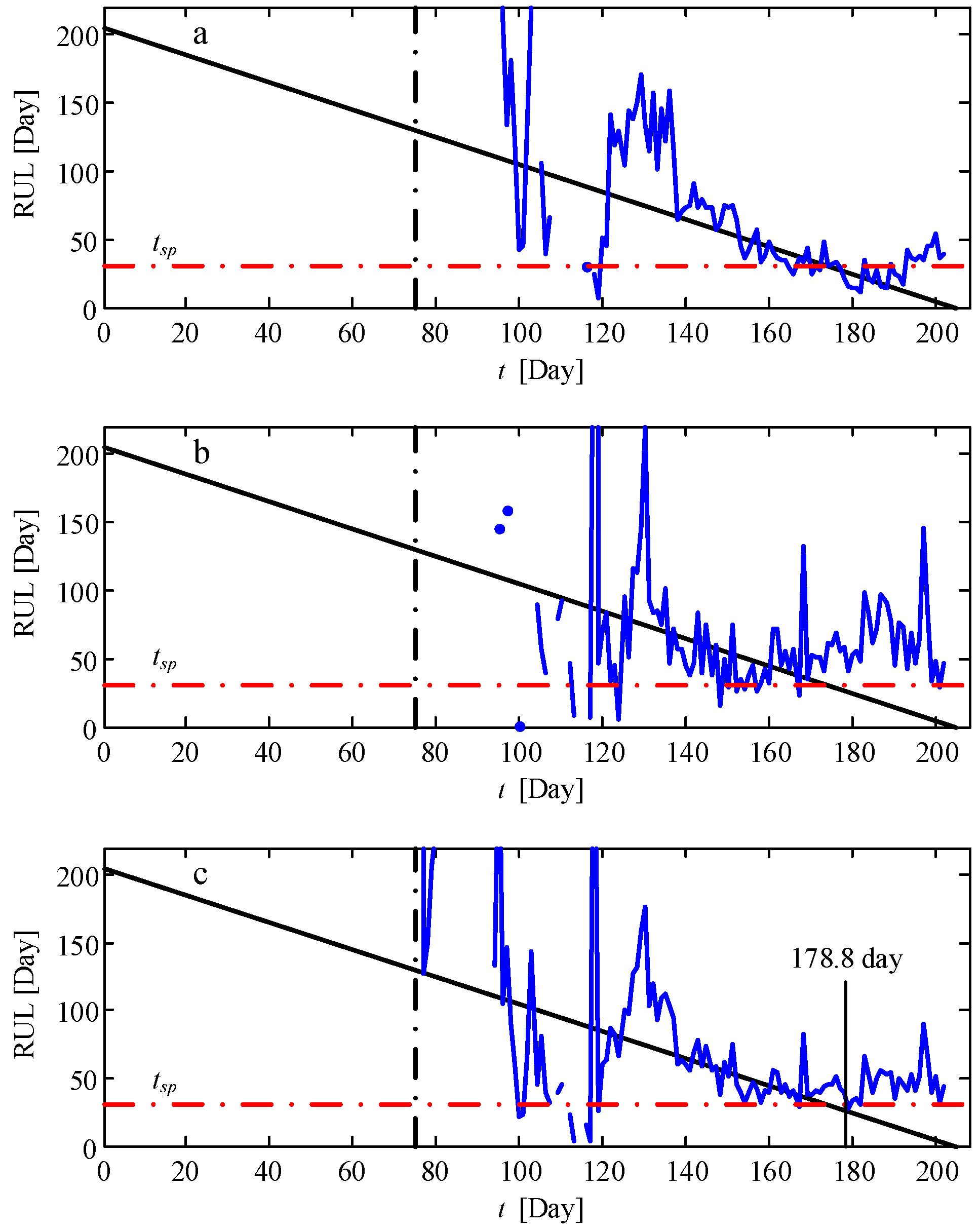
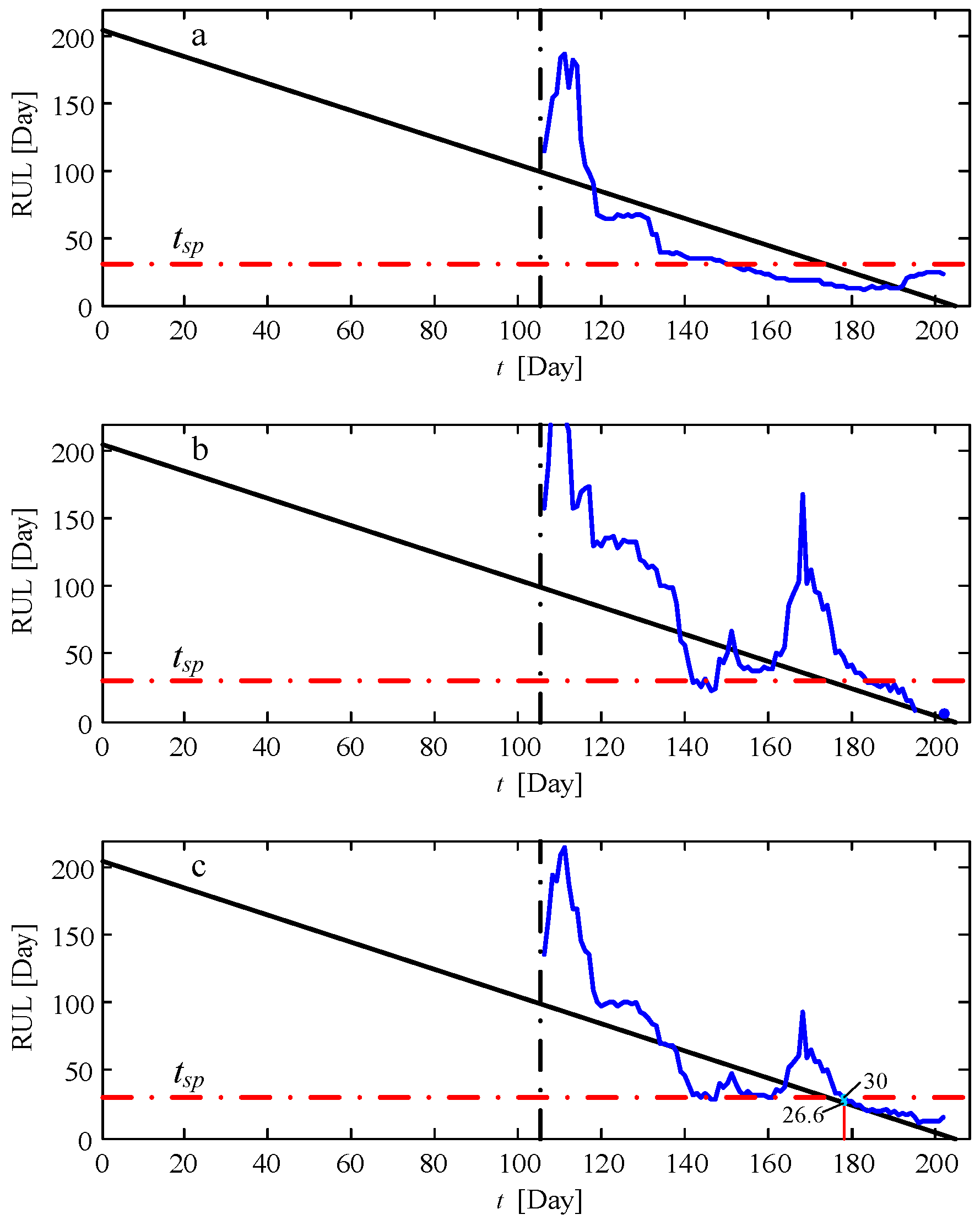
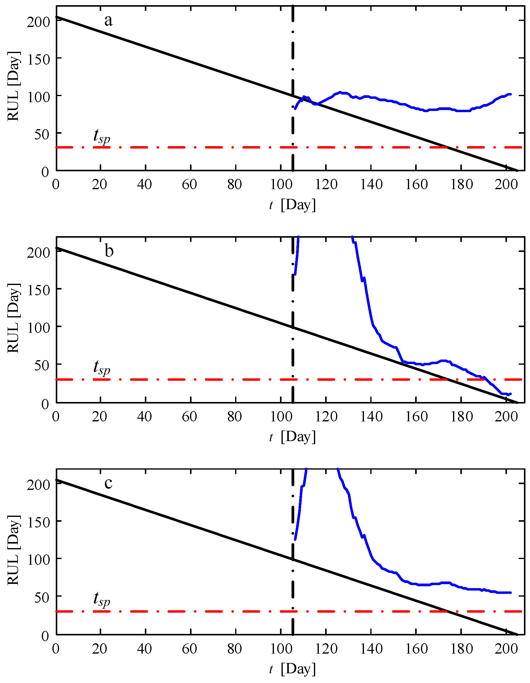
4.3. Prognosis of the Remaining Useful Life of the Faulty Bearing

The faulty bearing in the high speed shaft is near transducer 6 in Figure 1. However, the vibration amplitude of transducer 5 in Figure 5a is larger than the one of transducer 6 in Figure 5b, and the fault feature in Figure 6 is more obvious than in Figure 7. These are caused by different mounting positions of the two transducers. In the gearbox case, the stiffness of the location where transducer 5 is installed is less than that of the location of transducer 6. According to the vibration criterion VDI 3834 [22] for wind turbine gearboxes, the vibration amplitude of transducer 5 is too large to be a prognostic index. Therefore, transducer 6 is analyzed and regarded as the prognostic object in this paper.

Eight time features and four frequency features are calculated according to

Table 4. The statistical features in time and frequency domain. RMS: root mean square.

Features	Formulas
Mean ($\overline{x}$)	${\displaystyle {\sum }_{i=1}^N{x}_i}/N$
RMS ($x_{\mathrm{RMS}}$)	$\sqrt{{\displaystyle {\sum }_{i=1}^N{x}_i^2}/N}$
Variance ($x_{\mathsf{\sigma }}^2$)	${\displaystyle {\sum }_{i=1}^N{(x_i-\overline{x})}^2}/N$
Square root of amplitude ($x_r$)	${\left({\displaystyle {\sum }_{i=1}^N\sqrt{\left|x_i\right|}}/N\right)}^2$
Skewness factor	${\displaystyle {\sum }_{i=1}^N{\left(x_i-\overline{x}\right)}^3}/\left(N\cdot x_{\mathsf{\sigma }}^3\right)$
Kurtosis factor	${\displaystyle {\sum }_{i=1}^N{\left(x_i-\overline{x}\right)}^4}/\left(N\cdot x_{\mathsf{\sigma }}^4\right)$
Waveform factor	$x_{\mathrm{RMS}}/\overline{x}$
Margin indicator	$x_{\mathrm{RMS}}/x_r$
Energy of 1st frequency band	$\mathrm{sum}\left[X(1:f_s/8)\right]$
Energy of 2nd frequency band	$\mathrm{sum}\left[X(1+f_s/8:f_s/4)\right]$
Energy of 3rd frequency band	$\mathrm{sum}\left[X(1+f_s/4:3\cdot f_s/8)\right]$
Energy of 4th frequency band	$\mathrm{sum}\left[X(1+3\cdot f_s/8:f_s/2)\right]$

N is the length of each section data, X is the Fourier transform of vibration signal, and f_s is the sampling frequency.

. Among all the time features in Figure 8, the root mean square (RMS), variance and square root of amplitude represent an ascending tendency that can indicate the degradation process of the faulty bearing. VDI 3834 provides a warning and alarm limit for the drive train of wind turbines based on the statistics of vibration RMS [22], so RMS is selected to be the feature index in RUL estimation since it has a deterministic threshold. For the vibration signal from the HSS of wind turbine gearbox, 12 m/s² is selected as the failure threshold [22]. A fault feature selected in RUL estimation should be monotonically increasing or decreasing, which represents predictability. For the frequency features in Figure 9, the spectrum energy of the 3rd frequency band performs better than the other three frequency features, thus it is regarded as the second prognostic index. When the bearing is normal (from 0 to 75th day), the mean value and standard deviation in the 3rd frequency band are 2.51 and 0.76. The failure threshold of this feature index is set as 2.51 + 5 × 0.76 = 6.31. Five is chosen as the multiple based on statistical theory [23].

Figure 10 and Figure 11 show the adopted RMS and the energy of the 3rd frequency band with their threshold. From the 75th day when the bearing fault arises, the RUL estimation starts. First, the feature indexes between the 75th and 105th day are used to train a NN, and the next 30 days’ tendency is predicted using trained NN according to Figure 4, here m = 64 and n = 32. Next, the polynomial line is fitted on the basis of the training and predicted features. Finally, the RUL is estimated by calculating the intersection of the fitted line and the pre-defined threshold. After collecting one-day’s new data, the training dataset is updated, and the prognostic process continues until the end. Figure 10 and Figure 11 show the short-term predicted results and fitted lines after the 105th and 154th day.

According to Equations (8) and (9), the RUL of the faulty bearing is estimated as in Figure 12 where the solid lines are the true RULs of the bearing and the fluctuant curves are the predicted RULs. Figure 12a shows the RUL using RMS of the life cycle vibration signals as the prognostic index, Figure 12b shows the RUL using the 3rd frequency band and Figure 12c shows the final RUL combining the above two features. Figure 6 and Figure 7 indicate that bearing fault arises from the 75th day. The features between the 75th day and the 105th are used to train NN model, so the predicted RUL starts from the 105th day in Figure 12. At the beginning of predicted RUL after the 105th day, it is inaccurate since the failure time is far from the prediction starting time. As time goes on, the predicted RUL is approaching the true RUL, which shows a good prognostic result. A safe preparation time t_sp denoted by the dash dot line is defined as a time to prepare spare parts appropriately, neither delay the replacement of critical parts while failure happens nor generate unnecessary inventory. According to [24], the safety preparation time (critical condition in [24]) should be defined uniquely for different critical parts. Therefore, considering the transportation and replacement time, t_sp = 30 day is an applicable option for the maintenance of bearings in wind turbine gearbox. In Figure 12c, while the estimated RUL reaches t_sp, time pasts 178.15 days, so the true RUL is 204.75 − 178.15 = 26.6 days. The prognostic accuracy is (30 − 26.6)/26.6 = 12.78%, and it is sufficient to guarantee an effective maintenance.

The estimated RUL without short-term prediction is shown in Figure 13 where only the historical features are used to fit the polynomial line. Figure 13a shows the RUL using RMS of the life cycle vibration signals as the prognostic index, Figure 13b shows the RUL using the 3rd frequency band and Figure 13c shows the final RUL combining the above two features. Due to the lack of short-term prediction of Section 3.1, the degradation tendency of fault features cannot be well fitted. Therefore apparently, the estimation accuracy of the RUL in Figure 13 is lower than the proposed approach in Figure 12.

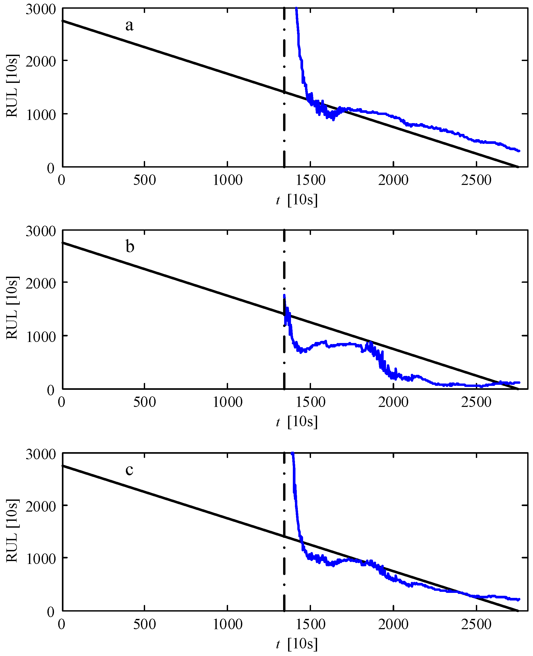
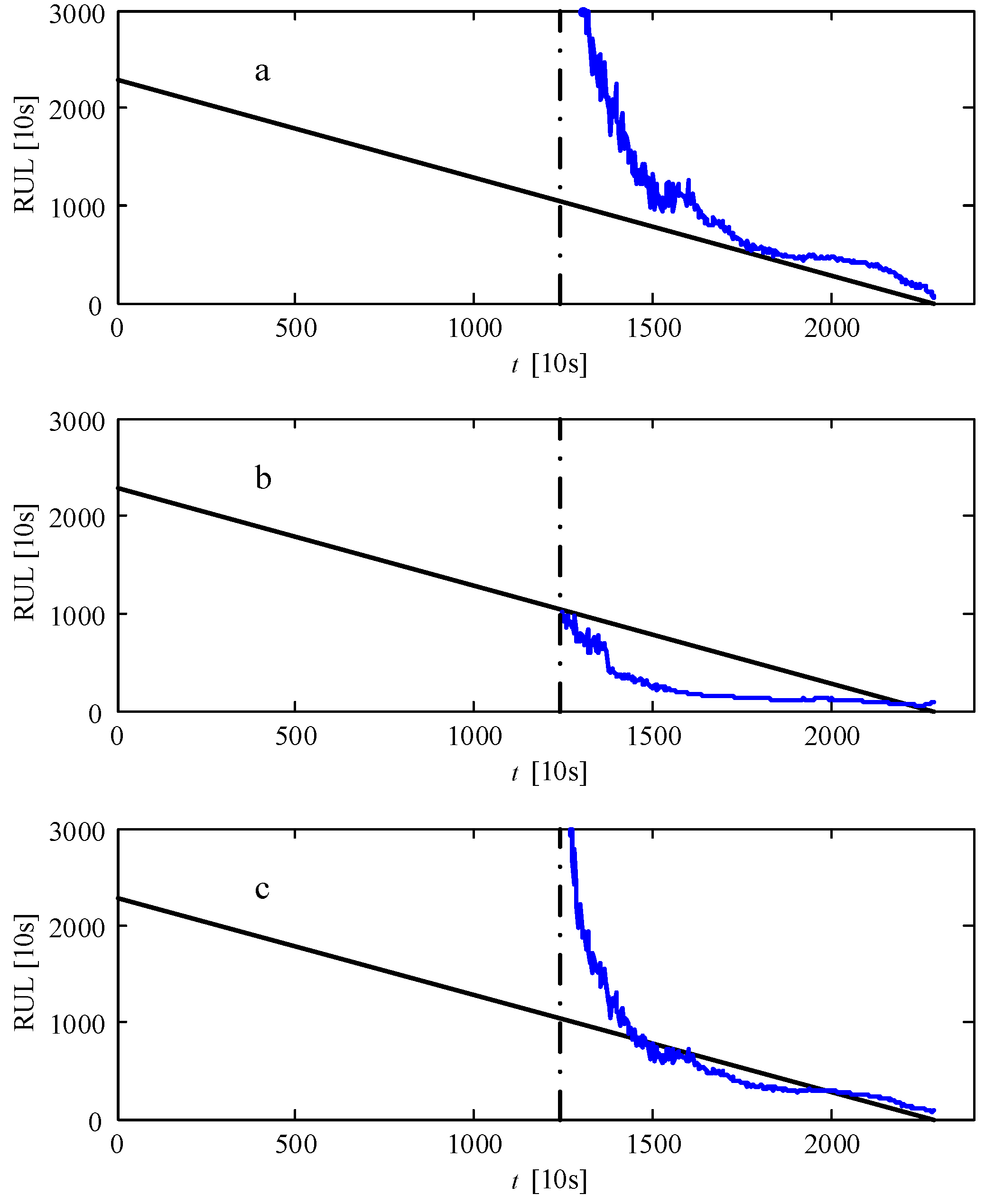
4.4. Comparision with Other Prognostic Method and Datasets

4.4.1. Echo State Network

An echo state network is one of the recurrent NNs that can solve any dynamical system with arbitrary accuracy [25]. It uses random recurrent networks to replace the hidden layer in traditional NNs and make the computation simple. Here, an echo state network is applied to predict the RUL of the bearings in wind turbine gearboxes. The prognostic procedure is similar to Figure 4, just substituting the NN by an echo state network to make the short-term tendency prediction. The number of input and output nodes in the echo state network is the same as in the NN described in Section 4.3. The result of the RUL estimation is shown in Figure 14.

In Figure 14, there are some discrete sections in the estimated RUL. The missing sections are caused by the negative solution of the inverse fitting curve in Equation (8). That indicates the RUL cannot be predicted at those times. In Figure 14c, while the estimated RUL reaches t_sp, time pasts 178.8 days, the true RUL is 204.75 − 178.8 = 25.95 days and the prognostic accuracy is (30 − 25.95)/25.95 = 15.61%. This prediction is accurate enough to schedule maintenance for the faulty bearing. However, compared with the results in Figure 12c, the estimated RUL using the echo state network in Figure 14c obviously fluctuates, representing a worse prognostic effectiveness. Especially after the safe preparation time, the estimated RUL gradually diverges from the true one.

4.4.2. Application of the Presented Approach of Remaining Useful Life Estimation to Experimental Dataset

Experimental datasets from PRONOSTIA [19] are used to further demonstrate the effectiveness of the proposed RUL estimation approach. Seventeen groups of life cycle vibration data are generated in this platform. Two datasets (bearing1_1, bearing1_3) with obvious increasing tendencies are selected to verify the RUL algorithm. Figure 15 show the RMS of the two datasets where 27,470 s and 22,880 s are set as the failure times. After those times, bearings enter into a severely damaged state, and they may fail at any time.

The RMS and the energy of the 3rd-frequency band are extracted as the feature indexes in the RUL estimation. The prognostic procedure is according to Figure 4.

For bearing1_1, the estimated RUL using RMS, the energy of the 3rd-frequency band, and the combination of the above two features are shown in Figure 16. At time 13,380 s, this bearing begins to show signs of fault and the prognostic procedure starts. The failure time is defined as 27,470 s. In Figure 16c, the predicted RUL matches well with the true RUL, thus illustrating the effectiveness of the proposed approach. The good performance of RUL estimation is also shown in Figure 17, the prognostic result of the dataset of bearing1_3.

5. Conclusions

RUL prognostic of critical subassemblies plays a significant role in the predictive maintenance of wind turbines. However, it is challenging due to the diversity of failures, the difficulty in extracting fault feature, and the instability of long-term predictions, etc.

The RUL estimation of the faulty bearings in wind turbine gearboxes in this paper involves fault diagnostics and RUL prognostics. Using analysis of the frequency spectrum, bearing faults can be distinctly detected and the start-point of RUL estimation can be determined. The RUL prognostic approach fuses NN-based short-term tendency prediction and polynomial fitting-based long-term tendency estimation.

Short-term prediction in RUL prognostics makes the fitted long-term tendency more practicable than the fitted result from pure historical features. Time and frequency features are individually selected to estimate the RUL of the bearings in wind turbine gearboxes. To overcome the fluctuation of individual features caused by varying amplitude loads, the time and frequency features are combined to obtain more accurate prognostic results than those available from the individual features. A safe preparation time is estimated with an acceptable error of 12.78%, which can benefit scheduling a reliable maintenance strategy for the bearings in wind turbine gearboxes.

References

1. Tian, Z.; Jin, T.; Wu, B.; Ding, F. Condition based maintenance optimization for wind power generation systems under continuous monitoring. Renew. Energy 2011, 36, 1502–1509. [Google Scholar] [CrossRef]
2. Byon, E.; Ntaimo, L.; Ding, Y. Optimal maintenance strategies for wind turbine systems under stochastic weather conditions. IEEE Trans. Reliab. 2010, 59, 393–404. [Google Scholar] [CrossRef]
3. Sarker, B.R.; Faiz, T.I. Minimizing maintenance cost for offshore wind turbines following multi-level opportunistic preventive strategy. Renew. Energy 2016, 85, 104–113. [Google Scholar] [CrossRef]
4. Yang, W.; Tavner, P.J.; Court, R. An online technique for condition monitoring the induction generators used in wind and marine turbines. Mech. Syst. Signal Process. 2013, 38, 103–112. [Google Scholar] [CrossRef]
5. Teng, W.; Ding, X.; Zhang, X.; Liu, Y.; Ma, Z. Multi-fault detection and failure analysis of wind turbine gearbox using complex wavelet transform. Renew. Energy 2016, 93, 591–598. [Google Scholar] [CrossRef]
6. Kusiak, A.; Verma, A. Analyzing bearing faults in wind turbines: A data-mining approach. Renew. Energy 2012, 48, 110–116. [Google Scholar] [CrossRef]
7. Dupuis, R. Application of oil debris monitoring for wind turbine gearbox prognostics and health management. In Proceedings of the Annual Conference of the Prognostics and Health Management Society, Portland, OR, USA, 10–16 October 2010.
8. Tchakoua, P.; Wamkeue, R.; Ouhrouche, M.; Slaoui-Hasnaoui, F.; Tameghe, T.; Ekemb, G. Wind Turbine Condition Monitoring: State-of-the-Art Review, New Trends, and Future Challenges. Energies 2014, 7, 2595–2630. [Google Scholar]
9. Tian, Z. An artificial neural network method for remaining useful life prediction of equipment subject to condition monitoring. J. Intell. Manuf. 2012, 23, 227–237. [Google Scholar] [CrossRef]
10. Tian, Z.; Wong, L.; Safaei, N. A neural network approach for remaining useful life prediction utilizing both failure and suspension histories. Mech. Syst. Signal Process. 2010, 24, 1542–1555. [Google Scholar] [CrossRef]
11. Ali, J.B.; Chebel-Morello, B.; Saidi, L.; Malinowskib, S.; Fnaiecha, F. Accurate bearing remaining useful life prediction based on Weibull distribution and artificial neural network. Mech. Syst. Signal Process. 2015, 56–57, 150–172. [Google Scholar]
12. Zio, E.; Peloni, G. Particle filtering prognostic estimation of the remaining useful life of nonlinear components. Reliab. Eng. Syst. Saf. 2011, 96, 403–409. [Google Scholar] [CrossRef]
13. Chen, C.; Vachtsevanos, G.; Orchard, M.E. Machine remaining useful life prediction: An integrated adaptive neuro-fuzzy and high-order particle filtering approach. Mech. Syst. Signal Process. 2012, 28, 597–607. [Google Scholar] [CrossRef]
14. Benkedjouh, T.; Medjaher, K.; Zerhouni, N.; Rechak, S. Remaining useful life estimation based on nonlinear feature reduction and support vector regression. Eng. Appl. Artif. Intell. 2013, 26, 1751–1760. [Google Scholar] [CrossRef]
15. Maio, F.D.; Tsui, K.L.; Zio, E. Combining relevance vector machines and exponential regression for bearing residual life estimation. Mech. Syst. Signal Process. 2012, 31, 405–427. [Google Scholar] [CrossRef]
16. Boskoski, P.; Gasperin, M.; Petelin, D.; Juricic, D. Bearing fault prognostics using Renyi entropy based features and Gaussian process models. Mech. Syst. Signal Process. 2015, 52–53, 327–337. [Google Scholar] [CrossRef]
17. Sikorska, J.Z.; Hodkiewicz, M.; Ma, L. Prognostic modelling options for remaining useful life estimation by industry. Mech. Syst. Signal Process. 2011, 25, 1803–1836. [Google Scholar] [CrossRef]
18. An, D.; Choi, J.H.; Kim, N.H. Prognostics 101: A tutorial for particle filter-based prognostics algorithm using Matlab. Reliab. Eng. Syst. Saf. 2013, 115, 161–169. [Google Scholar] [CrossRef]
19. Nectoux, P.; Gouriveau, R.; Medjaher, K.; Ramasso, E.; Morello, B.; Zerhouni, N.; Varnier, C. PRONOSTIA: An experimental platform for bearings accelerated life test. In Proceedings of the IEEE International Conference on Prognostics and Health Management, Denver, CO, USA, 18–21 June 2012.
20. Bishop, C.M. Pattern Recognition and Machine Learning; Springer: Berlin, Germany, 2006; Chapter 5. [Google Scholar]
21. D’Addona, D.M.; Matarazzo, D.; Ullah, A.M.M.S.; Teti, R. Tool wear control through cognitive paradigms. Procedia CIRP 2015, 33, 221–226. [Google Scholar] [CrossRef]
22. Measurement and Evaluation of the Mechanical Vibration of Wind Energy Turbines and Their Components—Onshore Wind Energy Turbines with Gears; VDI 3834; The Association of German Engineers: Duesseldorf, Germany, 2009.
23. Lyons, L. Discovering the Significance of 5σ. Available online: https://arxiv.org/pdf/1310.1284v1.pdf (accessed on 7 October 2013).
24. Le, B.; Andrew, J. Modelling wind turbine degradation and maintenance. Wind Energy 2016, 19, 571–591. [Google Scholar] [CrossRef]
25. Jaeger, H. Tutorial on Training Recurrent Neural Networks, Covering BPPT, RTRL, EKF and the “Echo State Network” Approach; GMD Report 159; German National Research Center for Information Technology: St. Augustin, Germany, 2002. [Google Scholar]
Figure 1. The drive train of wind turbines and the placement of transducers.
Energies 10 00032 g001
Figure 2. Structure of a wind turbine gearbox.
Energies 10 00032 g002
Figure 3. Neural network (NN) prediction model.
Energies 10 00032 g003
Figure 4. Process of remaining useful life (RUL) prognostic.
Energies 10 00032 g004
Figure 5. Temporal vibration signals: (a) transducer 5; and (b) transducer 6.
Energies 10 00032 g005
Figure 6. Waterfall of vibration signal from transducer 5.
Energies 10 00032 g006
Figure 7. Waterfall of vibration signal from transducer 6.
Energies 10 00032 g007
Figure 8. Time features: (a) mean; (b) RMS; (c) variance; (d) square root of amplitude; (e) skewness factor; (f) kurtosis factor; (g) waveform factor; and (h) margin indicator.
Energies 10 00032 g008
Figure 9. Frequency features: (a) spectrum energy of the 1st frequency band; (b) spectrum energy of the 2nd frequency band; (c) spectrum energy of the 3rd frequency band; and (d) spectrum energy of the 4th frequency band.
Energies 10 00032 g009
Figure 10. The RMS of transducer 6 with short-term predicted results and fitted lines.
Energies 10 00032 g010
Figure 11. The spectrum energy of the 3rd frequency band of transducer 6 with short-term predicted results and fitted lines.
Energies 10 00032 g011
Figure 12. The estimated RUL using the proposed approach: (a) using RMS of the life cycle vibration signals; (b) using the 3rd frequency band; and (c) combining the above two features.
Energies 10 00032 g012
Figure 13. The estimated RUL without short-term prediction: (a) using RMS of the life cycle vibration signals; (b) using the 3rd frequency band; and (c) combining the above two features.
Energies 10 00032 g013
Figure 14. The estimated RUL using echo state network: (a) using RMS of the life cycle vibration signals; (b) using the 3rd frequency band; and (c) combining the above two features.
Energies 10 00032 g014
Figure 15. RMS of life cycle vibration signals from PRONOSTIA [19]: (a) bearing1_1; and (b) bearing1_3.
Energies 10 00032 g015
Figure 16. The estimated RUL of bearing1_1 using the proposed approach: (a) using RMS of the life cycle vibration signals; (b) using the 3rd frequency band; and (c) combining the above two features.
Energies 10 00032 g016
Figure 17. The estimated RUL of bearing1_3 using the proposed approach: (a) using RMS of the life cycle vibration signals; (b) using the 3rd frequency band; and (c) combining the above two features.
Energies 10 00032 g017