Numerical Investigation of Terrain-Induced Turbulence in Complex Terrain by Large-Eddy Simulation (LES) Technique

Abstract

In the present study, field observation wind data from the time of the wind turbine blade damage accident on Shiratakiyama Wind Farm were analyzed in detail. In parallel, high-resolution large-eddy simulation (LES) turbulence simulations were performed in order to examine the model’s ability to numerically reproduce terrain-induced turbulence (turbulence intensity) under strong wind conditions (8.0–9.0 m/s at wind turbine hub height). Since the wind velocity and time acquired from the numerical simulation are dimensionless, they are converted to full scale. As a consequence, both the standard deviation of the horizontal wind speed (m/s) and turbulence intensity evaluated from the field observation and simulated wind data are successfully in close agreement. To investigate the cause of the wind turbine blade damage accident on Shiratakiyama Wind Farm, a power spectral analysis was performed on the fluctuating components of the observed time series data of wind speed (1 s average values) for a 10 min period (total of 600 data) by using a fast Fourier transform (FFT). It was suggested that the terrain-induced turbulence which caused the wind turbine blade damage accident on Shiratakiyama Wind Farm was attributable to rapid wind speed and direction fluctuations which were caused by vortex shedding from Tenjogadake (elevation: 691.1 m) located upstream of the wind farm.

1. Introduction

Recently, the number of accidents which have involved wind turbines constructed on complex terrain in the mountains is increasing rapidly. Recent studies by the author of the present study and others indicate that these investigated accidents are strongly associated with terrain-induced turbulence [1,2]. In these studies, terrain-induced turbulence is defined as “temporal and spatial fluctuations of airflow that are mechanically generated due to terrain irregularities.” Furthermore, the author of the present study classified terrain-induced turbulence roughly into two kinds.

The first kind is “extraordinary” terrain-induced turbulence, which is generated with the passage of a typhoon or a rarely occurring meteorological phenomena. That is, this kind of turbulence is terrain-induced turbulence that is commonly generated in wind directions that are different from the prevailing wind direction, and that occur infrequently throughout a year. It has been reported that this kind of terrain-induced turbulence caused a serious accident that involved cracks on the wind turbine blades and other damage [1].

The other kind of terrain-induced turbulence is “ordinary” terrain-induced turbulence, which is generated under the prevailing wind direction. This turbulence has caused reduced power output from wind turbines, and damage to the interior and exterior of wind turbines (e.g., the breakdown of yaw motors and yaw gears), which have become evident issues [2].

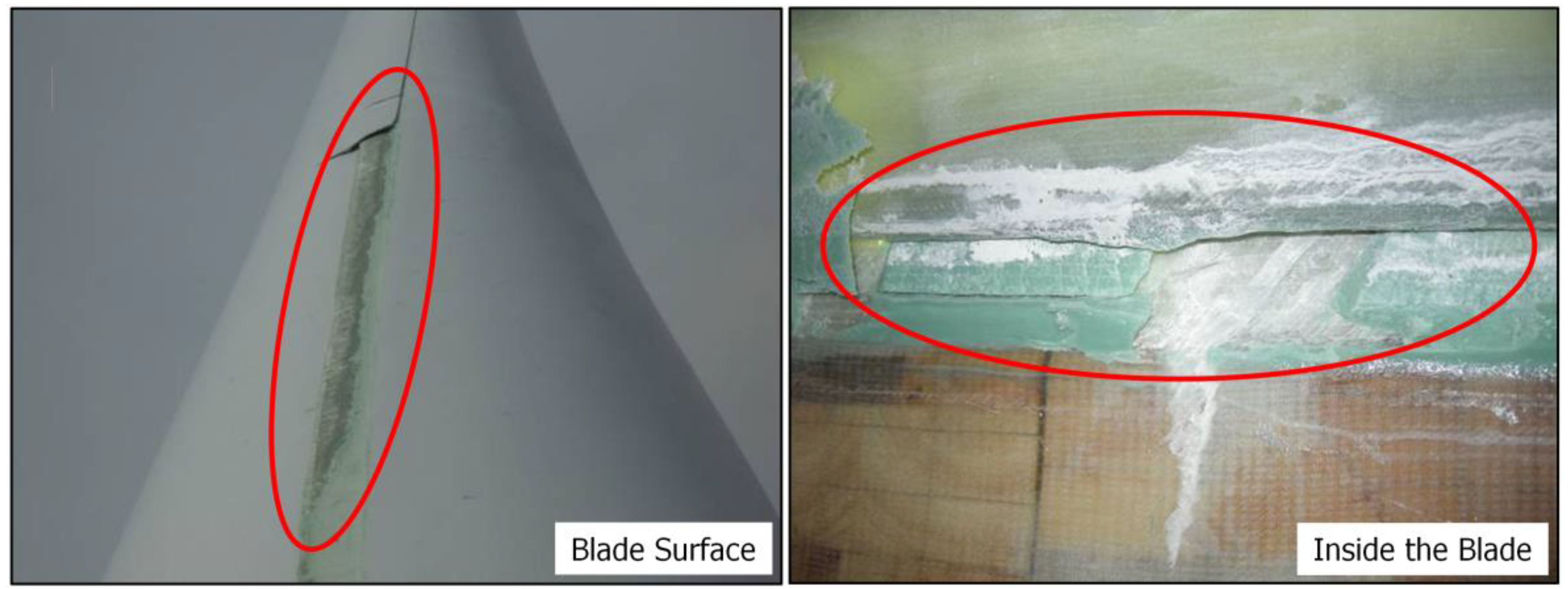
Uchida [1] investigated “extraordinary” terrain-induced turbulence. When Typhoon No. 0918 (Melor) passed the southern part of the main island of Japan between 7 and 8 October 2009, strong winds with extremely strong turbulence fluctuations were observed over the ridge of Mt. Shirataki and the surrounding ridges in Houhoku-cho, Shimonoseki City, Yamaguchi Prefecture, Japan. This strong wind caused damage to a turbine blade on Shiratakiyama Wind Farm owned by Kinden Corporation (Figure 1). Uchida [1] studied the cause of this accident by reconstructing the atmospheric phenomena occurring on spatial scales between a few meters and a few hundred kilometers using a computer simulation. In this study, the airflow field from the time of the accident was initially reconstructed in detail using a combination of a mesoscale meteorological model and RIAM-COMPACT, which is based on a large-eddy simulation (LES) turbulence model. Subsequently, the airflow fields in the vicinity of wind turbine blades were reconstructed separately using a Reynolds-averaged Navier-Stokes equations (RANS) turbulence model in order to evaluate the wind pressure on the wind turbine blades. For this analysis, the time-averaged flow field data from the LES simulation were used for the boundary conditions. Finally, stress exerted on the blades was calculated using a finite element method (FEM) with the RANS analysis results as the boundary conditions.

The results of the above analyses revealed that large values of stress occurred at the junction between the dorsal and ventral sides of the leading edge (LE) (the LE dorsal–ventral junction, hereafter), and that the locations at which these values occurred matched the locations of the actual damage. The static strength of the adhesive bond used for the LE dorsal-ventral junction is quite high. However, adhesive bonds will likely break when repeated loading, as the one discussed above, is applied to LE dorsal–ventral junctions as a result of low-cycle fatigue; that is, fatigue associated with approximately 10⁴ or fewer cycles for the number of cycles-to-failure. During the passage of Typhoon 0918, a large number of wind direction deviations were observed under high wind conditions. Therefore, it was surmised that damage such as cracks formed at the LE dorsal–ventral junction as a result of low-cycle fatigue, and this damage propagated further during subsequent wind turbine operation.

In contrast, Uchida [2] probed into “ordinary” terrain-induced turbulence by studying Taikoyama Wind Farm (located on Mt. Taikoyama, Nomura, Ine Town, Yosa District, Kyoto Prefecture, Japan). At this wind farm, at around 19:30 on 12 March 2013, a major accident occurred in which the nacelle and blades (hub height: approx. 50.0 m; weight: approx. 45.0 t) of Wind Turbine No. 3 fell to the ground as a result of a rupture of the tower in the vicinity of the tower top flange. Since the wind speed at the time of the accident was about 15.0 m/s, and this was within the design limit, investigations were conducted based on a standpoint that metal fatigue was the main cause of the accident. As a result of detailed investigations of the accident, the following was revealed: tensile stress on the welded joint between the tower shell and the tower top flange increased significantly because of the breakage of tower top bolts, which led to the formation of fatigue cracks on the internal wall of the tower shell in the vicinity of the weld toe. The formation of these fatigue cracks, in turn, caused the nacelle and blades to fall to the ground.

Detailed numerical wind simulation results for the prevailing wind direction showed that many wind velocity shears that deviated from those predicted by a power law occurred at all of the wind turbine sites, including Wind Turbine No. 3, the nacelle and blades of which fell to the ground. The simulation results also revealed that large wind direction deviations in the yaw direction of the wind turbines occurred frequently. Furthermore, the streamwise component of the wind velocity was relatively large, and the standard deviation of the vertical component of the wind velocity was large. The values of the standard deviation of the spanwise component of the wind velocity were approximately the same as those of the streamwise component of the wind velocity. From these findings, the following was conjectured. The exciting force on Wind Turbine No. 3 increased due to the effect of terrain-induced turbulence. As a result of the increased exciting force, additional load was imposed in the vicinity of the tower top flange, and thus increased metal fatigue in multiple bolts.

In light of the recent increase in wind turbine accidents such as the ones described above, laws and regulations about wind power generation in Japan have been reviewed and amended. Specifically, the Nuclear and Industrial Safety Agency of the Ministry of Economy, Trade, and Industry amended a part of the Ministerial Ordinance for Establishing Technical Standards for Wind Power Generation Facilities Based on the Electricity Business Act, Interpretations of Technical Standards, and the Rules for the Electricity Business Act. Regarding the “wind pressure” that is stipulated in Article No. 4 of the Ministerial Ordinance for Establishing Technical Standards for Wind Power Generation Facilities Based on the Electricity Business Act and that is relevant for examining safety in terms of wind turbine structures, it was specified by the Nuclear and Industrial Safety Agency that “wind pressure” is to be calculated by taking into account wind conditions at a wind turbine site that include extreme values of wind speed and turbulence fluctuations in the streamwise, spanwise, and vertical directions at the hub height of a wind turbine (27 June 2014).

As a result of this clarification on the use of wind conditions (turbulence) at a wind power generation facility, there is no doubt that the prediction and evaluation of turbulence intensity over complex terrain by computational fluid dynamics (CFD) such as LES and RANS will become increasingly important [3,4,5,6,7,8,9,10,11,12,13]. Generally, in RANS models, such as k–ε models, the standard deviation of the streamwise wind velocity which is attributable to terrain and/or surface roughness, ${\sigma }_u^{Surf}$, is calculated using the values of turbulence kinetic energy, k; then, the standard deviation of the streamwise wind velocity, ${\sigma }_u$, is calculated by taking into account the background atmospheric turbulence intensity, $I_a$ [14].

$${\sigma }_u^{Surf}=0.93\sqrt{k}$$

(1)

$${\sigma }_u=U\times \sqrt{{\left(\frac{{\sigma }_u^{Surf}}{U}\right)}^2+I_a^2}$$

(2)

where the background atmospheric turbulence intensity, $I_a$, is taken as 0.1. The standard deviations of the spanwise and vertical wind velocities are calculated automatically using the ratios of these standard deviations to ${\sigma }_u$ based on, for instance, an International Electrotechnical Commission (IEC) standard. However, this approach does not make it possible to evaluate the standard deviations of the three wind velocity components that result from turbulence structures that develop over complex terrain, and thus which deviate from those over flat, homogeneous terrain. In contrast, LES, which allows for unsteady simulations, does not involve the above-mentioned assumptions and makes it possible to directly evaluate the standard deviations of the three wind velocity components using time series data of the three wind velocity components as is the case for evaluations of the standard deviations with field wind observation data. Therefore, LES is a highly effective means to predict and evaluate turbulence intensity over complex terrain.

In the present study, field observation wind data from the time of the wind turbine blade damage accident at Shiratakiyama Wind Farm, which was investigated in Uchida [1], are analyzed in detail. In addition, a high-resolution LES turbulence simulation is performed by refocusing attention on the connection between the blade damage and the terrain-induced turbulence that caused the blade damage. Based on the results from this simulation, the numerical reproducibility of terrain-induced turbulence by the LES model is examined.

2. Shiratakiyama Wind Farm and Airflow Characteristics from the Time of the Blade Damage Accident

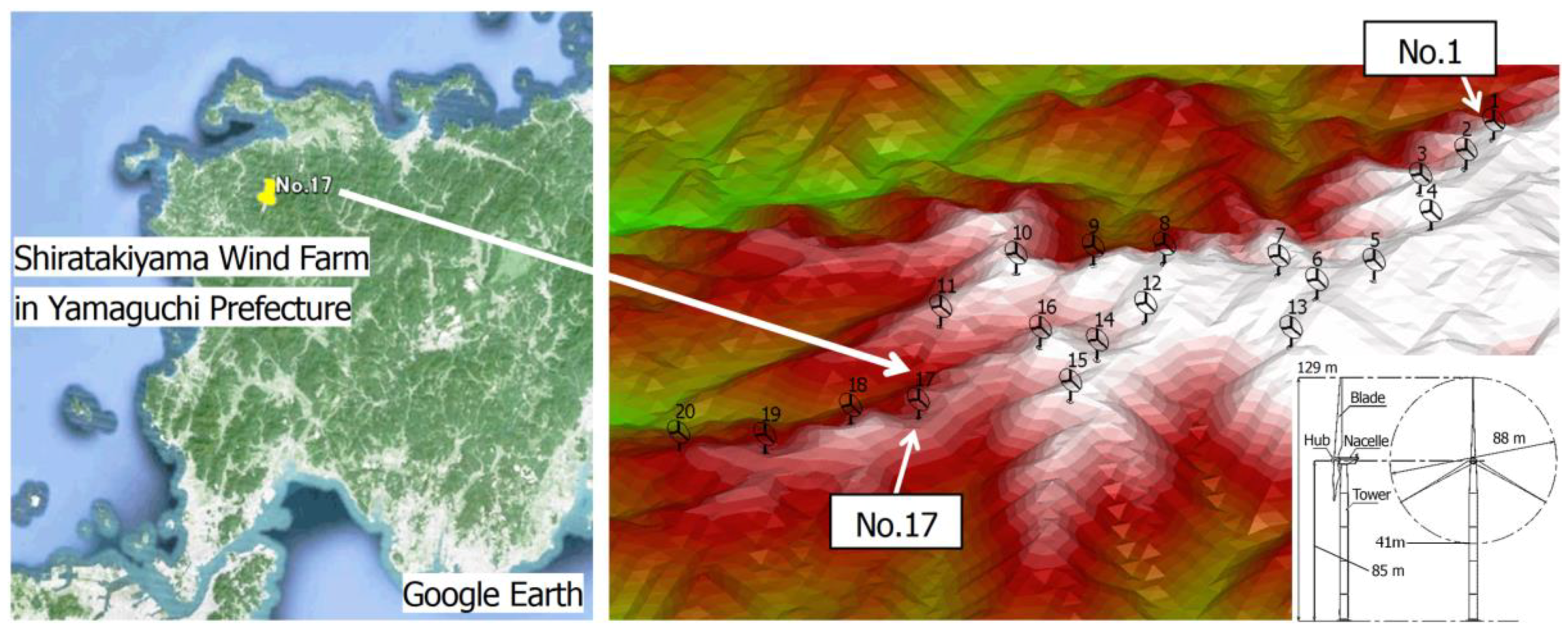
The Shiratakiyama Wind Farm owned by Kinden Corporation is located on a ridge near Mt. Shirataki in Houhoku-cho, Shimonoseki City, Yamaguchi Prefecture, Japan. On this wind farm, twenty 2500 kW wind turbines manufactured by General Electric Company (wind turbine hub height: 85.0 m; swept-area diameter: 88.0 m; height of the upper end of the swept area above the ground surface: 129.0 m; height of the lower end of the swept area above the ground surface: 41.0 m) are deployed (see Figure 2 and Figure 3).

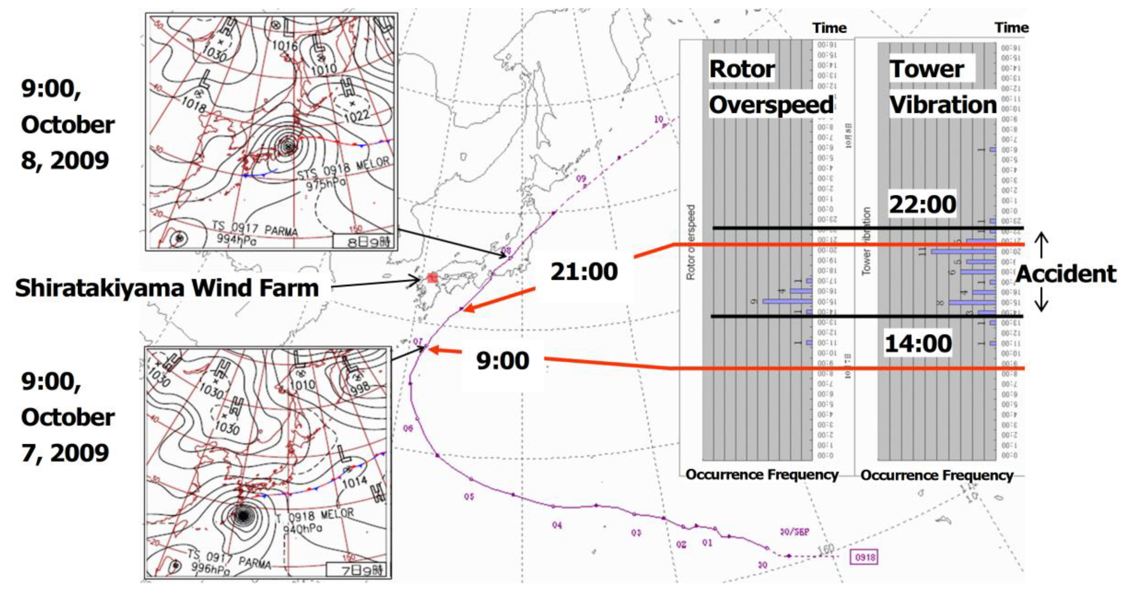
Figure 4 shows the trajectory of Typhoon No. 0918 (Melor), pressure charts from 9:00, 7 October 2009 and 9:00, 8 October 2009, and the number of wind turbine incidents on these two days. Generally, strong winds blow to the east of the direction of motion of a typhoon. However, on 7 October 2009, on which the blade damage accident occurred, the center of the typhoon was located to the south of the main island of Japan, as shown by the trajectory of the typhoon. Therefore, the position of Shiratakiyama Wind Farm on this day was in the range between north and west of the center of the typhoon. At that time, a steep horizontal pressure gradient (i.e., a zone with densely packed isobars extending from east to west) was present between the typhoon and the high pressure located to the north of the typhoon. As a result, the wind was flowing from the east around the typhoon to the north of the typhoon, which caused a strong north-easterly wind to flow into the site of the blade damage accident, causing the accident.

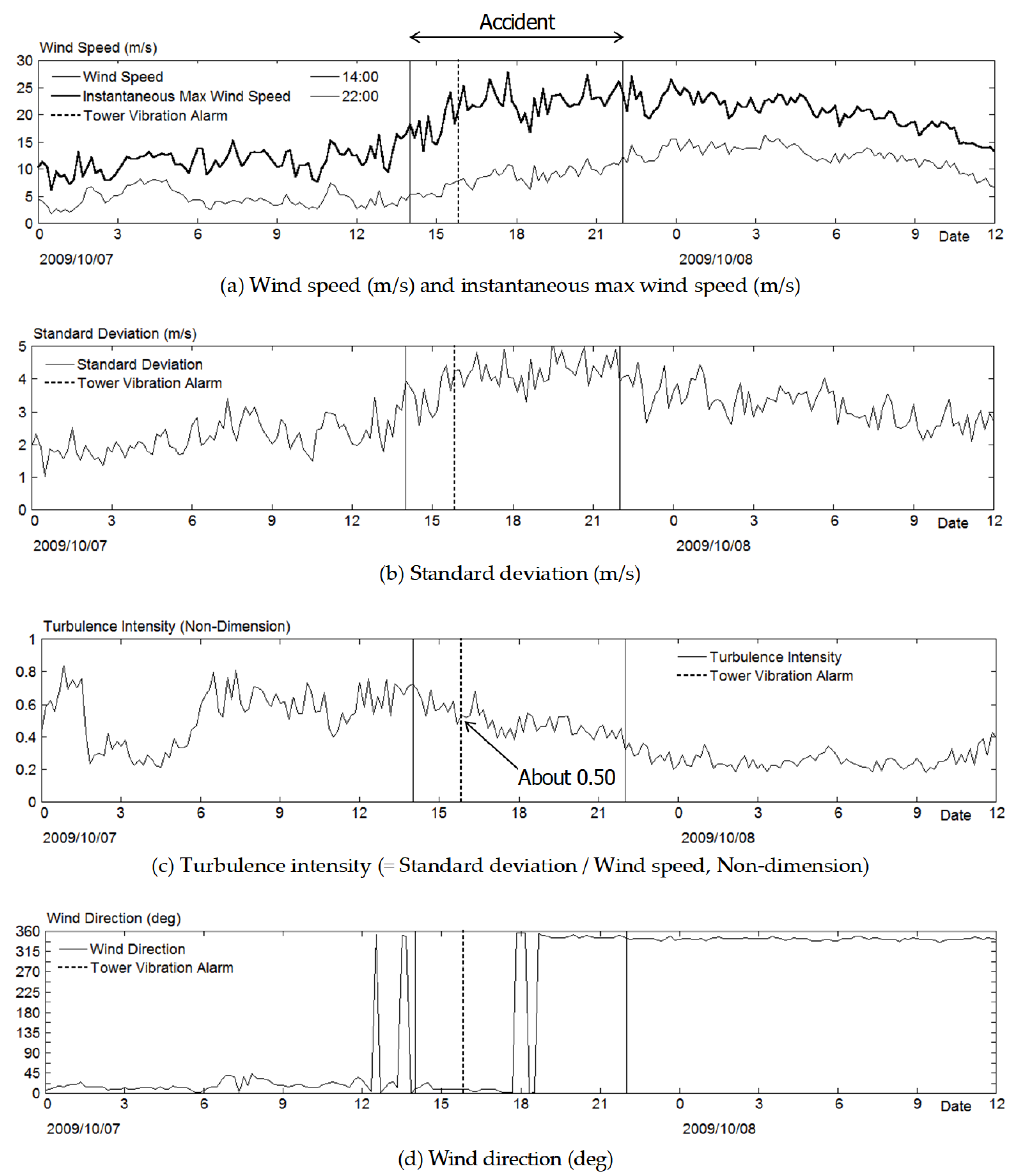
As indicated on Figure 4, the time period in which the wind turbine blade damage accident occurred was between 14:00 and 22:00 on 7 October 2009. In this time period, alarms for tower vibration, excessive rotation, and abnormalities in wind direction deviations were frequently set off for the wind turbines in operation. Furthermore, wind speed and wind direction deviations were subject to large fluctuations, which caused severe fluctuations in the rotor speeds and pitch angles of the wind turbine blades.

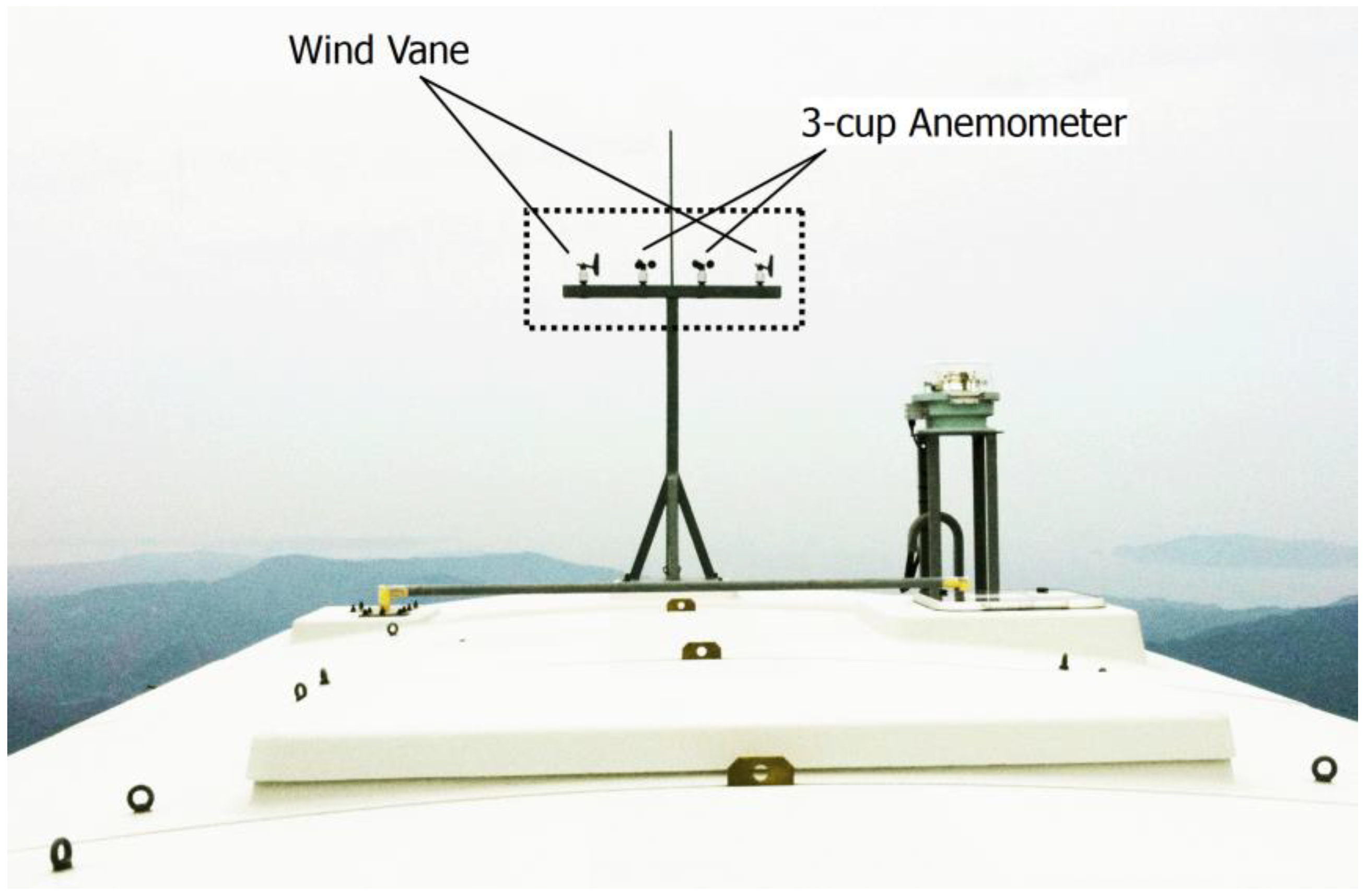
Figure 5 shows a photo of wind vanes and anemometers mounted on the top of the nacelle of a wind turbine No. 1. The field observation wind data used in the present study are those acquired from these wind vanes and anemometers.

Figure 6 shows time series data from one of the wind vanes and one of the anemometers mounted on the nacelle of Wind Turbine No. 17 (50.0 m above the ground surface). In Figure 6a–d, the horizontal axes indicate the time (Midnight, 7 October 2009 to noon, 8 October 2009). These figures also include indications of (1) the time period in which the wind turbine blade damage accident occurred (14:00–22:00, 7 October 2009), and (2) the start time of the tower vibration (15:50). On 7 October 2009, the wind speed started increasing gradually in the area of Shiratakiyama Wind Farm in the afternoon. As described earlier, at around 14:00, 7 October 2009, the time at which the wind turbine blade damage accident began, a north-easterly wind was flowing into the farm near the ground surface. As shown in Figure 6c, at the time at which the tower vibrations started (15:50), the turbulence intensity reached 0.50.

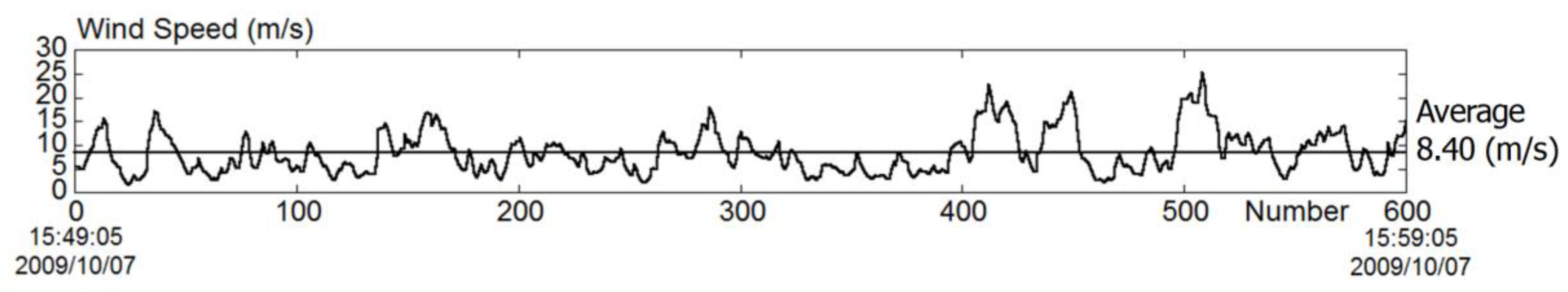
Figure 7 shows the time series of wind speed (1 s average values) for a 10 min period which includes the start time of the tower vibrations (15:50). It can be seen from this figure that the observed wind speed fluctuated significantly with periodicity. Concurrently with the significant wind speed fluctuations, very frequent wind direction deviations were also observed (not shown). The most frequent wind direction at Shiratakiyama Wind Farm is northerly, and it is rare that strong easterly or north-easterly wind flows into this wind farm, as in the case under investigation in the present study. As discussed in Uchida [1], when a strong northeasterly wind flows into Shiratakiyama Wind Farm, airflows characterized by rapid fluctuations in wind direction and speed (terrain-induced turbulence), which originate from a relatively large terrain feature located upwind of the wind farm, flow into the wind turbines.

Under strong wind conditions such as those described above, the pitch control of the wind turbine blades enters a state of not being able to respond appropriately to rapid wind velocity fluctuations. As a result, large amounts of wind pressure (wind load or stress) that exceed the wind pressure presumed at the time of design may be exerted on the LE dorsal–ventral junction. It was conjectured in Uchida [1] that, in the wind turbine accident at Shiratakiyama Wind Farm, repeated exertion of such wind pressure on the LE dorsal–ventral junction caused damage (cracks) at this junction due to low-cycle fatigue, and that this damage propagated further during subsequent wind turbine operation.

In the present study, a new high-resolution LES turbulence simulation was performed to investigate the numerical reproducibility of the terrain-induced turbulence that caused the wind turbine blade damage accident.

3. Overview of the Numerical Simulation Method

The present study employed the wind farm design tool called RIAM-COMPACT, which is based on a large-eddy simulation (LES) turbulence model [1,2,15,16,17,18,19,20,21,22,23,24,25]. This software simulates the local airflow with the use of a collocated grid arrangement in a general curvilinear coordinate system. For the governing equations of the flow, a filtered continuity equation for incompressible fluid (Equation (3)) and a filtered Navier-Stokes equation (Equation (4)) are used. In the present study, the LES was assumed to reproduce wind tunnel testing. Therefore, the effects of atmospheric stability associated with vertical thermal stratification of the atmosphere were neglected. In addition, as in Uchida [1,2], the effects of the surface roughness were taken into consideration by reconstructing surface irregularities in high resolution. The comparison between the RANS results and the present LES results are summarized in the latest article [15], and the prediction accuracy of the present LES approach by comparison with wind tunnel experiments are discussed in the article [25].

For the computational algorithm, a method similar to a fractional step (FS) method [26] was used, and a time marching method based on the Euler explicit method was adopted. The Poisson’s equation for pressure was solved by the successive over-relaxation (SOR) method. For the discretization of all the spatial terms, except for the convective term in Equation (4), a second-order central difference scheme was applied. For the convective term, a third-order upwind difference scheme was applied. The interpolation technique by Kajishima et al. [27] was used for the fourth-order central differencing that appeared in the discretized form of the convective term. For the weighting of the numerical diffusion term in the convective term discretized by third-order upwind differencing, α = 0.5 was used, as opposed to α = 3.0 from the Kawamura–Kuwahara scheme [28], in order to minimize the influence of numerical diffusion. For LES subgrid-scale modeling, the standard Smagorinsky model [29] was adopted with a model coefficient of 0.1 in conjunction with a wall-damping function:

$$\frac{\partial {\overline{u}}_i}{\partial x_i}=0$$

(3)

$$\frac{\partial {\overline{u}}_i}{\partial t}+{\overline{u}}_j\frac{\partial {\overline{u}}_i}{\partial x_j}=-\frac{\partial \overline{p}}{\partial x_i}+\frac{1}{Re}\frac{{\partial }^2{\overline{u}}_i}{\partial x_j\partial x_j}-\frac{\partial {\tau }_{ij}}{\partial x_j}$$

(4)

$${\tau }_{ij}\approx \overline{u_i^{\text{'}}{u}_j^{\text{'}}}\approx \frac{1}{3}\overline{u_k^{\text{'}}{u}_k^{\text{'}}}{\delta }_{ij}-2{\nu }_{SGS}{\overline{S}}_{ij}$$

(5)

$${\nu }_{SGS}={\left(C_s{f}_s\Delta \right)}^2\left|\overline{S}\right|$$

(6)

$$\left|\overline{S}\right|={\left(2{\overline{S}}_{ij}{\overline{S}}_{ij}\right)}^{1/2}$$

(7)

$${\overline{S}}_{ij}=\frac{1}{2}\left(\frac{\partial {\overline{u}}_i}{\partial x_j}+\frac{\partial {\overline{u}}_j}{\partial x_i}\right)$$

(8)

$$f_s=1-exp\left(-z^{+}/25\right)$$

(9)

$$\Delta ={\left(h_x{h}_y{h}_z\right)}^{1/3}$$

(10)

4. Overview of the Numerical Simulation Set-Up

The computational domain used in the present study extended over the space of 21.0 km (x) × 10.0 km (y) × 3.4 km (z), where x, y, and z are the streamwise, spanwise, and vertical directions, respectively. The maximum terrain elevation within the computational domain was 686.0 m, and the minimum terrain elevation was the sea surface (0.0 m). Terrain elevation data with 10.0 m and 50.0 m spatial resolutions from the Geospatial Information Authority of Japan (GSI) were used. The total number of computational grid points, 421 (x) × 201 (y) × 51 (z), was approximately 4.3 million, and the grid spacing was uniform (50.0 m) in both the x- and y-directions. 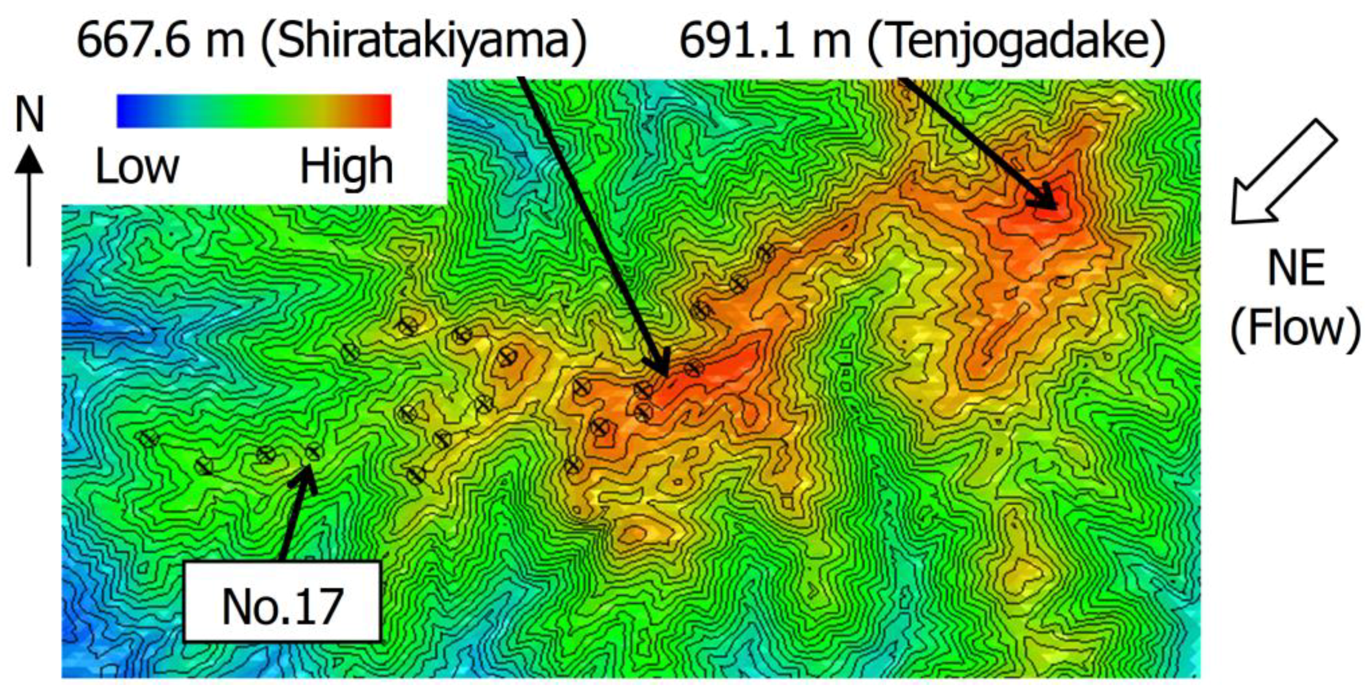Figure 8 shows a comparison of terrain configurations constructed from two datasets, i.e., 10.0 m and 50.0 m resolutions, for the area of Shiratakiyama Wind Farm. The comparison revealed no significant difference, and the accuracy of the reconstructed terrain was approximately the same between the two datasets. The grid spacing was non-uniform in the z-direction so that the density of grid points increased smoothly toward the ground surface. The minimum vertical grid spacing was 2.0 m. 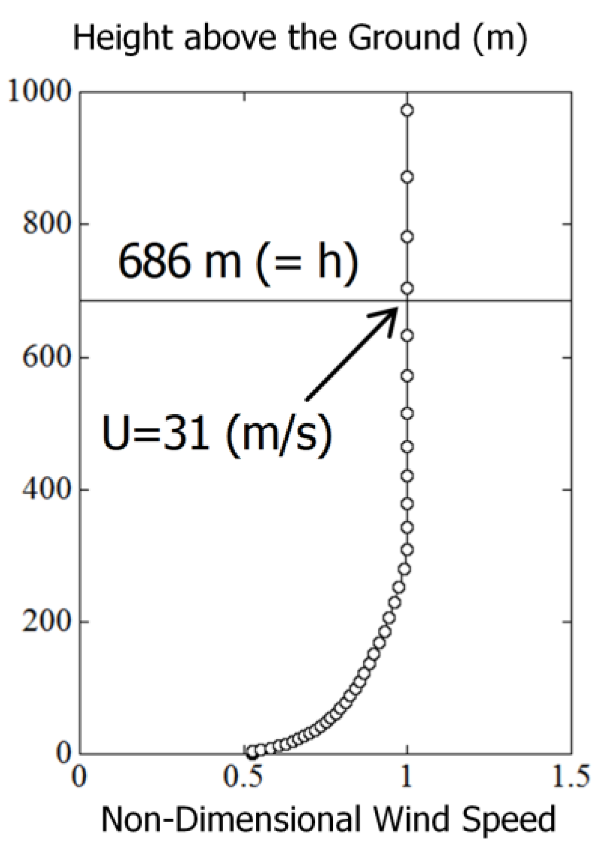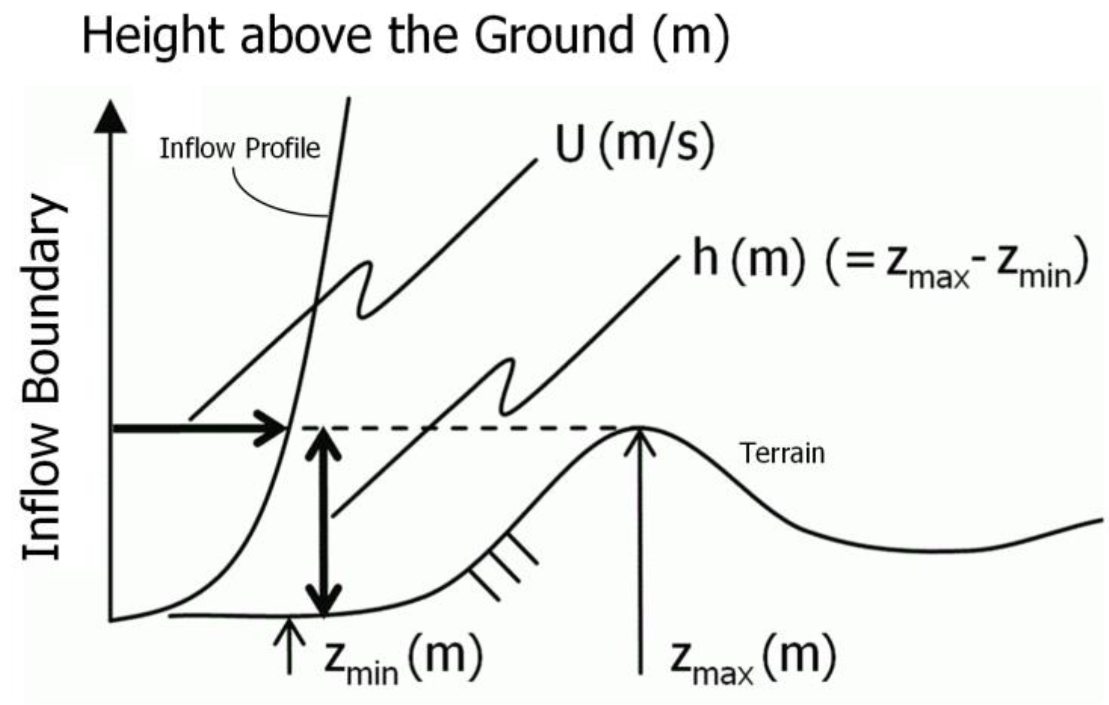An earlier study of the wind blade damage accident [1] conjectured that the accident occurred with a northeasterly wind. Therefore, the simulations in the present study were also performed for northeasterly wind conditions. Regarding the boundary conditions, the wind velocity profile applied at the inflow boundary was based on a commonly used empirical power law (see Figure 9). A power law index was set to 5. At the side and upper boundaries, free-slip conditions were applied, and convective outflow conditions were applied at the outflow boundary. On the ground surface, a non-slip boundary condition was imposed. The non-dimensional parameter Re in Equation (4) is the Reynolds number (=Uh/ν). For the simulations, Re = 10⁴ was used. Figure 10 illustrates the characteristic scales used in the present simulations: h is the difference between the minimum and maximum terrain elevations within the computational domain (=686.0 m), U is the wind velocity at the inflow boundary at the height of the maximum terrain elevation within the computational domain, and ν is the kinematic viscosity of air. The time increment is set to Δt = 2 × 10⁻³ h/U.

5. Results and Discussions Based on the Non-Dimensional Simulation Outputs

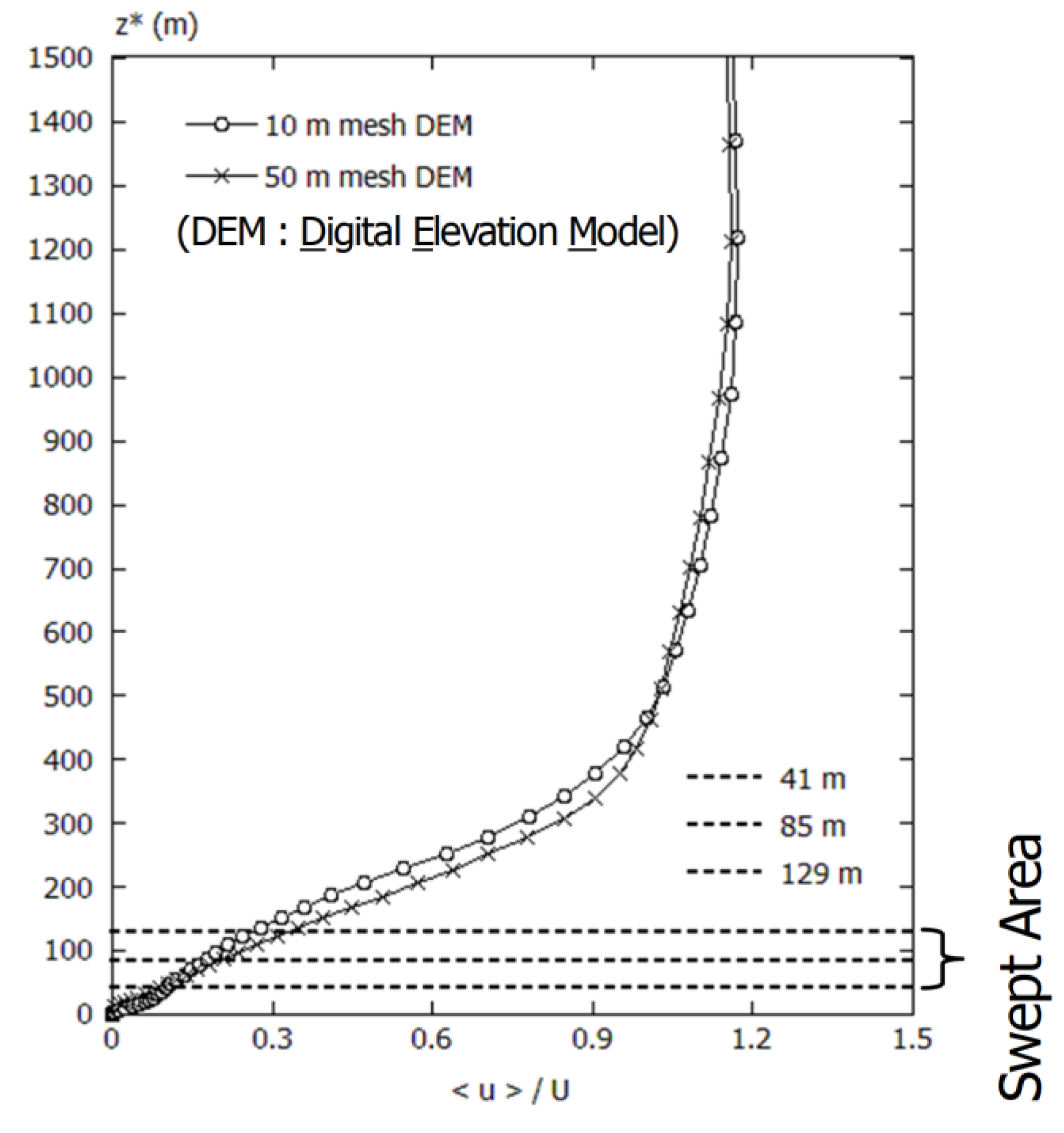
First, a comparison was made on the results from the simulations which used terrain elevation data with 10.0 m and 50.0 m resolutions from the Geospatial Information Authority of Japan (GSI). Figure 11 shows the vertical profiles of the mean streamwise wind velocity from the two simulations. Specifically, the plotted values were acquired by time-averaging (frame-averaging) the streamwise wind velocity at Wind Turbine No. 17 over the non-dimensional time period of t = 200.0–400.0. These values correspond to the output from a RANS model. The variable z* on the vertical axis represents the height above the terrain surface (m), and the horizontal axis represents the averaged streamwise wind velocity normalized by the inflow wind velocity U (m/s). As can be presumed from the fact that no significant differences existed between the two terrain datasets (see Figure 8), the tendencies of the results from the two simulations, including those plotted in Figure 11, were nearly the same. In light of this finding, further discussions are presented based on the results from the simulation, which used the 10.0 m resolution terrain elevation data.

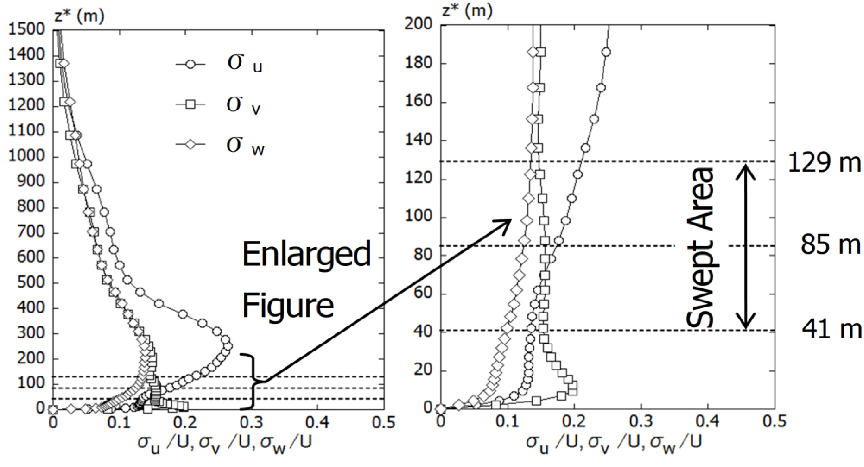
Figure 12 shows the vertical profiles of the standard deviations of the three wind velocity components at Wind Turbine No. 17. The standard deviations were calculated with respect to the time-averaged (frame-averaged) wind velocity components from the non-dimensional time period of t = 200.0–400.0. In the present study, the fluctuating wind velocity components (gusts) that are present in the observed inflow wind were not included in the inflow wind in the simulation; thus, only the airflow fluctuations of terrain-induced turbulence that were generated due to the terrain irregularities were evaluated. The left panel of Figure 12 shows the entire range, and the right panel of Figure 12 shows an enlarged view for the range of z* = 0.0–200.0 m. The left panel (entire range) indicates that the maximum value of the standard deviation of the x-component of the wind velocity occurred in the vicinity of z* = 300.0 m. The right panel (enlarged view) shows that the values of the standard deviations of the three wind velocity components were relatively large within the swept area of the wind turbine. In particular, it should be especially mentioned that the values for the y-component exceeded those for the x-component at the wind turbine hub height (=85.0 m) and below. This finding suggests the formation of an anisotropic turbulent flow field, in which the turbulent eddies are distorted significantly away from isotopic forms.

6. Results and Discussions Based on the Rescaled-Simulation Outputs

Based on the rescaled-simulation outputs, we tried to examine the model’s ability to numerically reproduce the terrain-induced turbulence (turbulence intensity) under strong wind conditions (8.0–9.0 m/s at wind turbine hub height). Since the wind velocity and time (t = 200.0–300.0, time step interval: 0.002, number of data values: approximately 50,000) acquired from the numerical simulation are dimensionless, they were converted to full scale with the procedure described below.

For the field observation wind dataset, scalar horizontal wind speed, U_scalar, was measured and recorded. This scalar horizontal wind speed, U_scalar, can be related to the horizontal wind speed acquired from the simulation as U_scalar = (u² + v²)^1/2, where u and v are the streamwise and spanwise wind velocities acquired from the simulation. As shown in Figure 7, the mean horizontal wind speed acquired from the field wind observations was 8.40 m/s. On the other hand, the non-dimensional mean horizontal wind speed from the numerical simulation was 0.27. Therefore, all of the wind velocity data values from the numerical simulation were multiplied by (8.40/0.27) to ensure that the mean horizontal wind speed from the numerical simulation would be equal to 8.40. Accordingly, the inflow wind velocity was set to approximately 31.0 m/s for the numerical simulation (see Figure 9). This value was in close agreement with the value of the wind velocity obtained from the mesoscale meteorological model in Uchida [1]. The non-dimensional time on the horizontal axis t (=200.0–300.0) was converted to full scale (s) based on T = t (h/U), where h = 686.0 m and U = 31.0 m/s for this case. As a result, the non-dimensional time interval of 100 was converted to approximately 2209 s (approximately 37 min) in full scale (time step interval: 0.044 s).

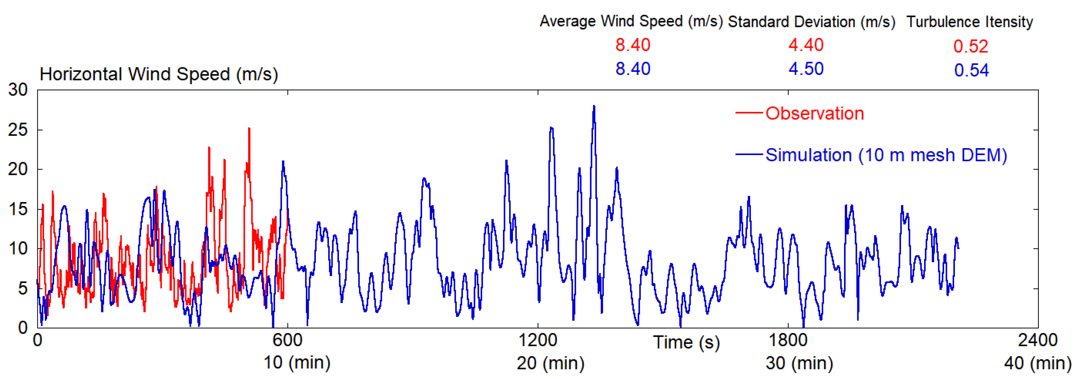
Figure 13 shows the temporal change (time series) of the horizontal wind speed from the hub height (85.0 m above the terrain surface) of Wind Turbine No. 17. In this figure, both the wind speed (m/s) on the vertical axis and time (s) on the horizontal axis represent those in full scale. Figure 13 also shows the field observation wind data, which are compared against the simulated wind data. These field observation wind data are the time series (1 s average values) from the 10 min period from Figure 7, which includes the time at which tower vibrations started (15:50). In Figure 13, the red solid line indicates field wind observation data (scalar horizontal wind speed) for 600 s (10 min), and the blue solid line indicates the horizontal wind speed calculated from the numerical simulation for approximately 2209 s (approximately 37 min). An examination of the numerical simulation results reveals the following. Rapidly fluctuating high-frequency components that were present in the field wind observation data were not fully reproduced in the simulation data. However, wind velocity fluctuations with very short periodic cycles which were attributable to the generation of terrain-induced turbulence, were reproduced for the most part. As a consequence, both the standard deviation of the horizontal wind speed (m/s) and turbulence intensity evaluated from the field observation and simulated wind data were successfully in close agreement (see numerical value shown in Figure 13). In order to obtain the time series with the above-mentioned periodicity, the settings of the parameters that are discussed below (i.e., horizontal grid resolution and time increment) were particularly important.

When strong north-easterly winds flow into Shiratakiyama Wind Farm, airflow characterized by rapid fluctuations in wind direction and speed (terrain-induced turbulence), which originate from a relatively large terrain feature located upwind of the wind farm, flow into the wind turbines. Therefore, it is necessary to accurately reproduce (1) a relatively large-scale terrain feature that is present upwind of the wind farm, and (2) the three-dimensional structure of the terrain-induced turbulence that is generated due to the terrain features, by sufficiently resolving the turbulence both temporarily and spatially. To achieve this goal, a grid resolution of approximately 50.0 m is required for the horizontal cross sections. Furthermore, in order to capture the unsteady fluid properties of terrain-induced turbulence, a sufficiently small time increment (Δt = 2 × 10⁻³ h/U in the present study) was required.

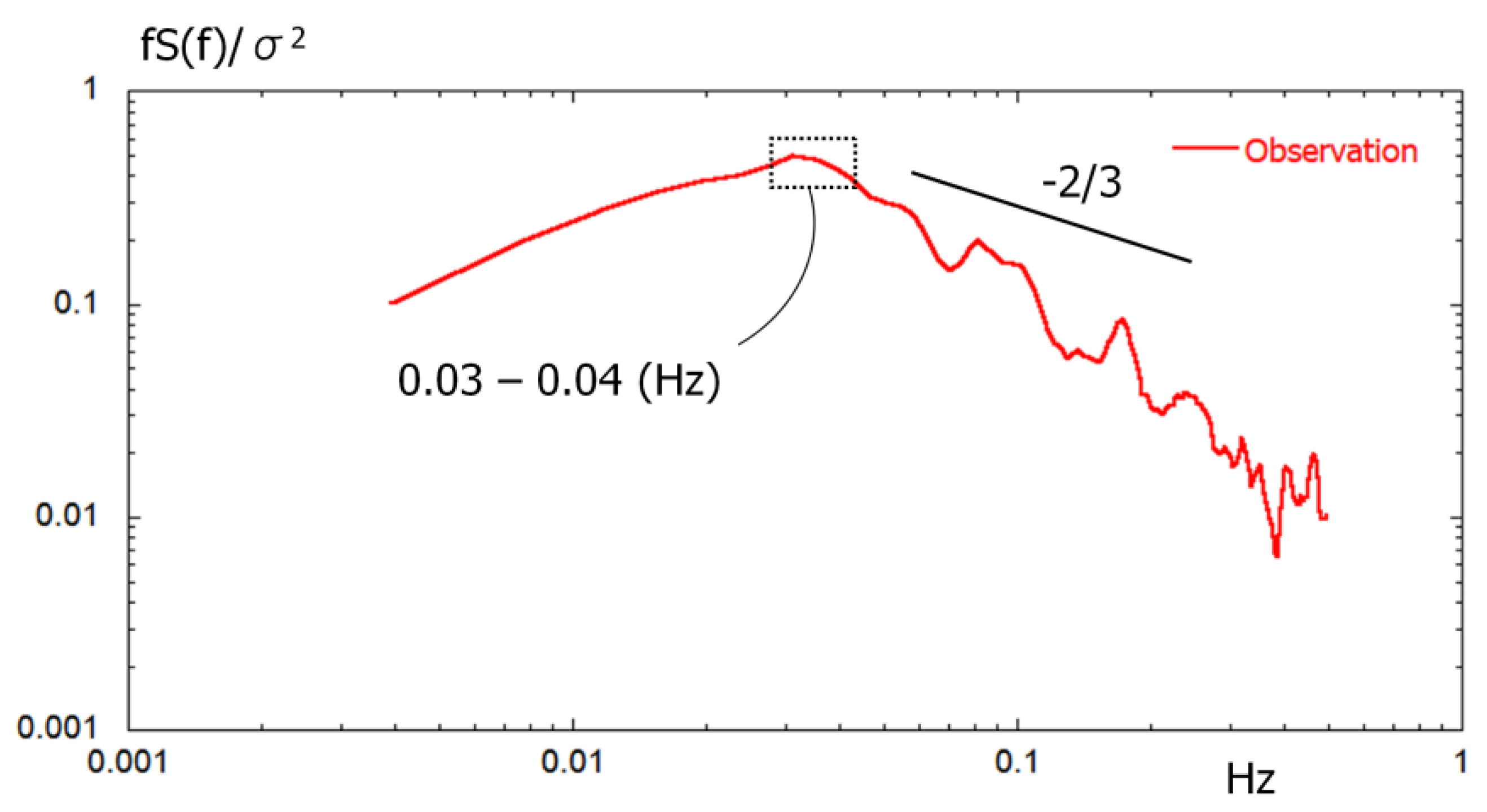
Finally, to investigate the cause of the wind turbine blade damage accident on Shiratakiyama Wind Farm, a power spectral analysis was performed on the fluctuating components of the observed time series data of wind speed (1 s average values) for a 10 min period (total of 600 data), indicated by a red line in Figure 13 by using a fast Fourier transform (FFT). The obtained results of this spectral analysis are shown in Figure 14. Here, the observed time series data (red line) shown in Figure 13 is the same as the data shown in Figure 7. The observed time series data of wind speed (1 s average values) for a 10 min period (total of 600 data), indicated by a red line shown in Figure 13, was divided into a 256 dataset. Then, spectral analysis was performed on the divided time series dataset, and a standard triangular window was also applied. In Figure 14, the vertical axis shows the power spectra, which is non-dimensionalized by the frequency f (Hz) and standard deviation σ (m/s), and the horizontal axis shows the frequency f (Hz). By using the dominant frequency from Figure 14, f = 0.04 Hz, the elevation of Tenjogadake, h = 691.1 m (see Figure 8), and the choice of the inflow wind velocity U = 31.0 m/s together yields 0.89 for the non-dimensional frequency, Strouhal number (St) (=f h/U). This value nearly agrees with the value of the vortex shedding frequency, St = 0.87, which was obtained from wind tunnel experiments with simple topography (a two-dimensional ridge and a three-dimensional isolated hill) [24]. Thus, it is likely that the terrain-induced turbulence that caused the wind turbine blade damage accident on Shiratakiyama Wind Farm was attributable to rapid wind speed and direction fluctuations, which were caused by vortex shedding from Tenjogadake (elevation: 691.1 m) located upstream of the wind farm.

7. Conclusions

In the present study, field observation wind data from the time of the wind turbine blade damage accident on Shiratakiyama Wind Farm, which was studied by Uchida [1], were analyzed in detail. In parallel, high-resolution LES turbulence simulations were performed in order to examine the model’s ability to numerically reproduce terrain-induced turbulence.

First, a comparison was made between terrain elevation data with 10.0 m and 50.0 m spatial resolutions from the Geospatial Information Authority of Japan (GSI). When a uniform grid spacing of 50.0 m was used for the horizontal grid for the airflow calculation, the accuracy of the simulation results was approximately the same between the simulations which used the two datasets. Furthermore, in order to capture unsteady fluid properties of terrain-induced turbulence, a sufficiently small time increment (Δt = 2 × 10⁻³ h/U) is required. Here, h is the difference between the minimum and maximum terrain elevations within the computational domain; U is the wind velocity at the inflow boundary at the height of the maximum terrain elevation within the computational domain.

Secondly, vertical profiles of the standard deviations of the three wind velocity components at Wind Turbine No. 17 were examined based on the non-dimensional simulation outputs. This examination revealed that the value of the standard deviation for the y-component of wind velocity exceeded that for the x-component of wind velocity at the wind turbine hub height (=85.0 m) and below.

Thirdly, based on the rescaled-simulation outputs, we try to examine the model’s ability to numerically reproduce terrain-induced turbulence (turbulence intensity) under strong wind conditions (8.0–9.0 m/s at wind turbine hub height). Since the wind velocity and time acquired from the numerical simulation are dimensionless, they are converted to full scale. As a consequence, both the standard deviation of the horizontal wind speed (m/s) and turbulence intensity evaluated from the field observation and simulated wind data are successfully in close agreement.

Finally, to investigate the cause of the wind turbine blade damage accident on Shiratakiyama Wind Farm, a power spectral analysis was performed on the fluctuating components of the observed time series data of wind speed (1 s average values) for a 10 min period (total of 600 data) by using a fast Fourier transform (FFT). It was suggested that the terrain-induced turbulence that caused the wind turbine blade damage accident on Shiratakiyama Wind Farm was attributable to rapid wind speed and direction fluctuations that were caused by vortex shedding from Tenjogadake (elevation: 691.1m) located upstream of the wind farm.