Energy Commodity Price Forecasting with Deep Multiple Kernel Learning


1
Department of Business Administration, National Changhua University of Education, Changhua 50074, Taiwan
2
School of Business Administration, Hubei University of Economics, Wuhan 430205, China
3
Research Center of Hubei Logistics Development, Hubei University of Economics, Wuhan 430205, China
4
Institute for Development of Cross-Strait Small and Medium Enterprise, Wuhan 430205, China
*
Authors to whom correspondence should be addressed.
Energies 2018, 11(11), 3029; https://doi.org/10.3390/en11113029
Submission received: 12 September 2018
/
Revised: 31 October 2018
/
Accepted: 1 November 2018
/
Published: 5 November 2018
(This article belongs to the Special Issue 10 Years Energies - Horizon 2028)
Abstract
:Oil is an important energy commodity. The difficulties of forecasting oil prices stem from the nonlinearity and non-stationarity of their dynamics. However, the oil prices are closely correlated with global financial markets and economic conditions, which provides us with sufficient information to predict them. Traditional models are linear and parametric, and are not very effective in predicting oil prices. To address these problems, this study developed a new strategy. Deep (or hierarchical) multiple kernel learning (DMKL) was used to predict the oil price time series. Traditional methods from statistics and machine learning usually involve shallow models; however, they are unable to fully represent complex, compositional, and hierarchical data features. This explains why traditional methods fail to track oil price dynamics. This study aimed to solve this problem by combining deep learning and multiple kernel machines using information from oil, gold, and currency markets. DMKL is good at exploiting multiple information sources. It can effectively identify the relevant information and simultaneously select an apposite data representation. The kernels of DMKL were embedded in a directed acyclic graph (DAG), which is a deep model and efficient at representing complex and compositional data features. This provided a solid foundation for extracting the key features of oil price dynamics. By using real data for empirical testing, our new system robustly outperformed traditional models and significantly reduced the forecasting errors.
1. Introduction
Crude oil is the world’s largest energy commodity and is actively traded internationally. The welfare of oil-importing and oil-producing economies are heavily influenced by fluctuations in oil prices, especially when they are unexpectedly large and persistent. As indicated by Abosedra and Baghestani [1], “sharp increases in crude oil prices adversely influence economic growth and accelerate inflation for oil importing economies. Large fall in crude oil prices will generate serious budgetary deficit problems for oil exporting countries”. Accurate oil price forecasting is appealing and important. Nevertheless, in modern time series analysis it is a very difficult task owing to its complex dynamics. Many researchers have tried to develop models to maximize forecasting accuracy. However, until now, they have not achieved a satisfactory level of performance from their models. The failure of traditional approaches is derived from their model setting. The model forms adopted are usually linear and parametric (Atsalakis and Valavanis [2,3], Fan and Li [4]), which are not flexible enough to track fast changing price dynamics. This study aims to solve this problem by developing a new strategy that combines the advanced deep learning and multiple kernel methods.
Oil price forecasts are important for related business operations, and they have great influences on many sectors of the economy. For example, these forecasts are used to determine airfares for airline companies, planning capacity for utility companies, shipping fees in the logistics industry, and product prices in the petrochemical industry. Referring to prior research (Bahrammirzaee [5], Fan and Li [4], Krollner et al. [6]), time series forecasting techniques can be divided into the three groups: (1) statistical or econometric models; (2) machine learning, artificial intelligence, and soft computing; (3) hybrid models that combine the above two methods. The typical models include the auto-regressive moving average (ARMA) (or the auto-regressive integrated moving average (ARIMA)) used in statistics, and the generalized auto-regressive conditional heteroscedasticity (GARCH), which is used in econometrics. Among ARMA and GARCH, there are many new ideas and improved models that have been developed recently for oil price forecasting. For example, Gupta and Wohar [7] forecasted oil and stock returns with a Qual VAR (Qualitative Vector Autoregressive) model. Gavriilidis et al. [8] examined whether the inclusion of oil price shocks of different origin as exogenous variables in a wide set of GARCH-X models improved their volatility forecasts. Herrera et al. [9] employed high-frequency intra-day realized volatility data to evaluate the relative forecasting performances of various econometrics models, such as the RiskMetrics, GARCH, asymmetric GARCH, fractional integrated GARCH, and Markov switching GARCH models. Morana [10] developed a semiparametric approach for short-term oil price forecasting. With respect to machine learning, artificial intelligence, and soft computing, traditional models include neural networks, genetic algorithms, and fuzzy logics. There are also many newly developed methods in this field. For example, Ding [11] developed a novel decompose-ensemble methodology with the AIC-ANN (Akaike information criterion-artificial neural network) approach for crude oil forecasting. Yu et al. [12] proposed a neural network ensemble learning paradigm based on empirical mode decomposition (EMD) to forecast crude oil prices.
In the third group, many hybrid models integrate the strengths of both methods to enhance their predictions. For example, Naderi et al. [13] developed a novel approach by using a meta-heuristic bat algorithm to optimally combine four predictors including the least square support vector machine (LSSVM), genetic programming (GP), ANN, and ARIMA in an integrated equation. Safari and Davallou [14] proposed a hybrid combination of the exponential smoothing model (ESM), ARIMA, and the nonlinear autoregressive (NAR) model in a state space model framework, in which the time-varying weight of the proposed hybrid model was determined by Kalman-Filter. Li et al. [15] proposed a method integrating ensemble empirical mode decomposition (EEMD), adaptive particle swarm optimization (APSO), and relevance vector machine (RVM) to predict crude oil prices. Wang et al. [16] used a linear ARIMA to correct the nonlinear metabolic grey model (NMGM) forecasting residuals to improve forecasting accuracy in China’s foreign oil dependence. Xiao et al. [17] developed a hybrid model based on a selective ensemble for energy consumption forecasting in China. Drachal [18] tried to find the time-varying drivers of spot oil price in a dynamic model averaging framework. Iranmanesh et al. [19] proposed a mid-term energy demand forecasting system by hybrid neuro-fuzzy models.
Recently, support vector machines (SVMs, Vapnik [20]) have been developed to enhance traditional neural networks. Kernel methods (Schoelkopf et al. [21]), the core of SVMs, have also received a lot of attention. In general, artificial intelligence and similar approaches are nonlinear, nonparametric, and adaptive in their model forms. They are flexible to track complex price dynamics, and thus usually outperform statistical methods. Another weakness of statistical models is related to their assumption that random variables follow a normal or other kind of distribution, which is limited because real data is not stationary and their dynamics change with time. Time-varying coefficient or distribution models in statistics are also insufficient, because their model settings are parametric. The dimensionality of their function space is finite, limited, and not flexible enough to track fast changing dynamics.
Due to the rapid development of the Internet and information technology, global financial markets are highly correlated. Oil is both an important energy commodity and a financial instrument that is heavily traded in global markets. Upon reviewing the research in oil or financial price predictions (Ding et al. [22], Iranmanesh et al. [19], Khashman and Nwulu [23], Liu et al. [24], Wang et al. [25], Xie et al. [26], Yu et al. [12]), we can confirm that machine learning or artificial intelligence approaches usually outperform statistical and econometric methods. However, there are still some weaknesses associated with machine learning or artificial intelligence approaches. Previously, kernel methods have been prolific, theoretical, and algorithmic machine learning frameworks. The success of kernel methods depends on good data representation or kernel design, and this has resulted in a lot of research that focuses on kernel design, which is adapted to specific data types. Conversely, there are also several generic kernel-based algorithms for typical learning tasks. The strength of SVMs is that they use structural risk to regularize model complexity, which leads to excellent generalization properties in out-sample forecasting. The mathematical formulation of an SVM is ideal because its objective function is convex with a unique solution. Consequently, the solution searching or parameter optimization algorithms are easier than those in neural network (NN) models. The kernels are typically hand-crafted and fixed in advance, and the roles of the kernel in an SVM can be divided into two parts: (1) it defines the similarity between two examples, and (2) it simultaneously acts as a regularization for the objective function.
Hand-tuning kernel parameters is difficult, as the appropriate sets of features need to be selected and combined. On the other hand, traditional SVMs are based on a single kernel, whereas in real-life applications data comes from multiple sources, and therefore, the representation by a single kernel is not sufficient. The combination of multiple kernels is a good solution; however, determining the process to combine them presents another problem. Lanckriet et al. [27] sought to address this problem and proposed an idea to learn the multiple kernels from training data. Their solution was to learn the target kernels as a linear combination of given basis or local kernels. Following Lanckriet et al. [27], various multiple kernel learning (MKL) formulations and modifications have been proposed. The success of MKL stems from the fact that using multiple kernels can enhance the interpretability of the decision function, and thus improve performance (Lanckriet et al. [27]). However, the number of the basis kernels that we need to consider is exponential in the dimension of the input space. Considering this decomposition for MKL directly is intractable. To address the issue of selecting basis kernels more efficiently, Bach [28,29] proposed a useful framework to design the MKL kernels. Owing to the fact that data features of modern time series are complex, compositional, and hierarchical, using the natural hierarchical (or deep) structure of the problem for the kernel design of MKL is a good solution. The suggestion made by Bach [28,29] involves embedding the kernels in a directed acyclic graph (DAG). The kernels embedded in a DAG form provide an excellent deep representation of the data features. Another contribution from Bach [28,29] is the proposal to perform high-dimensional kernel selection through a graph-adapted sparsity-inducing norm. Using the norm, the selection can be completed in polynomial time in the number of selected kernels.
Recently, deep learning (DL, Bengio et al. [30], Schmidhuber [31]) or deep representations (DR) have become very popular. As opposed to task-specific algorithms, DL aims to learn the data representation. Consequently, DL is also known as deep structured learning or hierarchical learning. In machine learning methods, DL has become the new trend in overcoming complex data mining problems. As previously mentioned, kernel methods are usually shallow models that cannot fully represent or capture complex, compositional, and hierarchical data features. This study aimed to combine the strengths of DL (or DR) and MKL. The kernels used in this study were embedded in a hierarchical directed acyclic graph, which is a deep representation form for real data. In the past few years, DL has become very popular in many fields of computer science, and the most recognized applications are in computer vision and natural language processing. With the advancement in storage technology, there are considerable quantities of labeled data available for training a model. This allowed us to learn large numbers of model parameters in DL without having to be concerned about overfitting. Another factor contributing to the success of DL is the rapid development of the Graphics Processing Unit (GPU). The computing power of the GPU grows very fast, whereas traditional complex DL model using CPU (Central Processing Unit) training requires weeks of computations. The training can be completed in a day on a GPU (see, e.g., He et al. [32], Ioffe and Szegedy [33], Krizhevsky et al. [34], Simonyan and Zisserman [35]). This study sought to bridge kernel methods and deep representations and ideally achieve the best of both worlds.
The remainder of this paper is organized as follows: Section 2 reviews the weaknesses and strengths of prior research, including the support vector regression (a type of SVMs), feedforward neural network (FFNN), radial basis functions (RBF) neural network, general regression neural network (GRNN), and DLs. Section 3 describes the proposed model. Section 4 introduces the real data we used to test the model, and discusses the empirical results. Finally, Section 5 is the conclusion.
2. Weaknesses and Strengths of Prior Research
2.1. Support Vector Regression
Based on the structured risk minimization (SRM) principle, support vector regression (SVR) seeks to minimize an upper bound of the generalization error, instead of the empirical error as in other neural networks. The concept of SVR is to find suitable support vectors in the margin and build the model according only to a subset of the training data. In the past, SVMs have achieved great performance in various applications, yet in some cases it was not satisfactory. SVMs need to overcome the following drawbacks: (1) Similar to NN models, the optimization algorithm needs to tune a large number of model parameters. The general strategy is to employ genetic algorithms (GA) or particle swarm optimization (PSO) algorithms to search for the best parameters (Huang and Wang [36], Ren and Bai [37]). Despite the fact that the objective function of an SVM is convex and has a unique solution, the parameter space is highly nonlinear and non-convex. Typical optimization (or tuning) algorithms are not very effective for searching in the parameter space. Although searching for optimal parameters by GA (or PSO) is an effective solution, this is time consuming and computationally intensive. (2) In high-dimensional data, an SVM also cannot get rid of the curse of dimensionality (Bellman [38]). For large-scale input data, the dimension of input space is very large, and the distribution of data points becomes very sparse. This results in a sharp deterioration in the SVM’s performance. (3) The representation of an SVM is not compact and concise, and it generally cannot produce sparse models. For example, in a system of identification, Drezet and Harrison [39] demonstrated that the model built by an SVM is not always parsimonious. (4) To make an SVM successful in many areas of application, the choice of a good kernel and features is very important and relies heavily on data processing experience.
2.2. Feedforward Neural Network
The notion of artificial neural networks was derived from biological neural networks. The neurons process information through a non-linear sigmoid function, and consequently, NNs are effective at non-linear data modeling. The strengths of NNs are in modeling complex relationships between inputs and outputs and finding patterns in data. However, there are also certain weaknesses in NN models including: (1) they depend on a large number of model parameters; (2) the solution space of NN is not convex, and the optimization algorithm is often trapped into local minima in the training; (3) the training of NN usually tends to be over-fitting, which results in a poor out-sample generalization; and (4) traditional NNs are shallow models, and thus their representation is insufficient. These problems are partially addressed by the technique of kernel methods or support vector machines.
2.3. Radial Basis Function and Generalized Regression Neural Networks
The radial basis function neural network (RBFNN) is in a special class of neural networks that consists of an input layer, a hidden layer, and an output layer. The neurons in the hidden layer of an RBF contain Gaussian transfer functions whose settings makes the outputs inversely proportional to the distance from the center of the neuron. The Generalized regression neural network (GRNN) is a variation of the RBFNN. GRNNs represent an improved technique to the neural networks based on nonparametric regression, and every training sample represents the mean to a radial basis neuron. GRNN can be used for regression, prediction, and classification and can also be a good solution for online dynamical systems. Similar to RBFNN, GRNN has the following advantages: (1) high accuracy in the estimation because it uses Gaussian functions; (2) single-pass learning so backpropagation would not be required; and (3) it can resist and handle noises in the inputs. However, there are still some disadvantages in GRNN, for example, there is no optimal method to improve it, and its size grows fast with the input dimension, which is computationally expensive.
2.4. Deep Learning
Deep learning is good at feature extractions and representations. It has achieved a remarkable performance breakthrough in several fields (such as speech recognition, natural language processing, and computer vision). In particular, convolutional neural network (CNN) architectures produce state-of-the-art performance on a variety of image analysis tasks. Currently, the weakness of DL is that most of DL research focused on dealing data with 1D, 2D, or 3D Euclidean spaces. However, most data from energy or financial markets lies on high-dimensional non-Euclidean manifolds. Generalizing deep learning methods to non-Euclidean structured data becomes very important. Applying differential geometry to generalize DL is a good solution. The generalizing (or geometric) deep learning can thus be applied to a variety of domains, such as network analysis, computational social science, computer graphics, and so on. Another weakness of DL is that their computation is quite heavy. We need multiple GPUs or cloud computing to accelerate the computation.
3. Deep (or Hierarchical) Multiple Kernel Learning
Kernel methods are popular learning frameworks and the basis of the approach can be stated as follows: through non-linear transformations, we can transform the input space to a larger and potentially infinite-dimensional feature space. Typically, the feature space is a reproducing kernel Hilbert space (RKHS), which is a space of functions in which point evaluation is a continuous linear functional. The advantage of RKHS is that it is more flexible and rich for feature representations than original input space. Via representer theorems, with the kernel function and appropriate regularization by Hilbertian norms, we can consider larger and potentially infinite-dimensional feature spaces without computing the coordinates of data in that space, but rather by simply computing the inner products between the images of all pairs of data in the feature space. This approach is called the “kernel trick”, which is computationally cheaper than the explicit computation of the coordinates. This has led to several studies on kernel design adapted to specific data types and generic kernel-based algorithms for many learning tasks.
In practical applications, data comes from multiple sources. Classical kernel machines are based on a single kernel, which is not capable of representing complex data sources. Consequently, it is more desirable to construct learning machines based on combinations of multiple kernels. The approach suggested by Bach [28,29] proposed a large feature space that is the concatenation of smaller feature spaces, and for real-life application, considered a positive definite kernel that can be expressed as a large sum of positive definite basis or local kernels. After the construction, we can apply multiple kernel learning to select among these kernels. However, directly applying multiple kernel learning in this decomposition is intractable because the number of these smaller kernels increases exponentially in the dimension of the input space. In order to overcome the difficulty in basis kernel selections, Bach [28,29] made an arrangement so that these small kernels could be embedded in a DAG, which happens to be a hierarchical structure that is effective at deep representations.
The following description of DMKL follows Bach [28,29]. For the problem to consider predicting a random variable Y from a random variable X, we defined and to be spaces of X and Y. Given n observations , the empirical risk in the estimation of a function f from X to R can be defined as , where l is a loss function.
Graph-Structured Positive Definite Kernels
To construct a larger kernel, , we assumed that this positive definite kernel is the sum, over an index set V, of basis kernels ; namely, for all , we have . For each , let’s denote and as the feature space and feature map of , i.e., , respectively. Consequently, the larger feature map and larger feature space of k can be expressed as the concatenation of the feature maps for each kernel , i.e, and . The learning algorithm of MKL tried to find for a certain to form a predictor function , which is equivalent to find jointly for , and .
The goal of this research was to perform kernel selection among the kernels . In order to accelerate the searching, we only considered specific subsets of V. We limited the basis kernels to be embedded in a graph, and as described by Bach [28], “instead of considering all possible subsets of active (relevant) vertices, we are only interested in estimating correctly the hull of these relevant vertices”.
We assumed that the input space can be factorized into p-components , and that there are p sequences of length of kernels , , such that the larger kernel . Thus we had a sum of kernels, that could be computed efficiently as a product of p sums. In this scenario, the products of kernels was equivalent to interactions between certain variables. The basis kernels embedding in a DAG implies that an interaction will be selected only after all sub-interactions are already selected. The framework of DAGs are particularly suited to deep feature representations and non-linear variable selection, and especially for the polynomial and Gaussian kernels.
In considering the linear kernel, , where stands for inner product; the full kernel is then equal to . Please note that this is not exactly the usual polynomial kernel. Typical polynomial kernels, , are multivariate polynomials of total degree less than q. Another example is the product of the Gaussian kernel, , which is also known as all-subset Gaussian kernel. ANOVA (analysis of variance) kernel is also famous in research. It is shown as follows:
The optimal hierarchical multiple kernel learning could be formulated as the following minimization problem:
where is the structured block -norm; are positive weights and is the descendant set of v (Since we are only interested in the hull of the selected elements , the hull of a set I is characterized by the set of v, such that , i.e., hull(I) = . In our context, we are hence looking at selecting vertices for which .). Penalizing by such a norm will indeed impose that some of the vectors are exactly zero, thereby leading to sparse solutions.
4. Experimental Results and Analysis
4.1. Data Sets Used for The Research
In modern society, our economy heavily depends on the energy sector. Investors all over the world pay attention to oil prices, which are one of the most important global economic variables. Energy markets are closely correlated with financial markets and are therefore economically linked. In determining which variables to include in our study, gold and oil are two kinds of commodities to hedge against inflation. In addition, since both gold and oil are globally traded in U.S. dollars, the currency markets should also be considered. Typically, the U.S. dollar is more sensitive to oil than gold. Consequently, this study proposed to consider the possible economic and financial linkages between the oil, gold, and currency markets. The markets for oil and gold have been extensively studied; however, in this analysis, we attempt to bring together these three markets and use recent methodologies to uncover the emerging relationships.
The testing data used in this study include five major crude oil spot prices: West Texas Intermediate (WTI), Brent, Forties, Dubai, and Oman. Brent and Forties are the reference for crude oil in the North Sea, WTI is the reference for the America, and Dubai and Oman are the references for the Middle East. This study aimed to forecast these crude oil spot prices, while taking the economic and financial linkages among oil, gold, currency markets into account. This analysis included the gold prices (New York), and the exchange rate between the U.S. dollar (USD) and the Taiwanese dollar (TWD) to enhance the predictions. In total, we had 5 crude oil spot prices (WTI, Brent, Forties, Dubai, and Oman), 2 financial prices (the gold prices and the U.S. exchange rate), and for every variable we considered 2 time lags. Consequently, there were 14 ((5 + 2) × 2 = 14) input time series in our model. The data covered the period from 1 May 2009 to 31 December 2010, and comprised of 435 daily observations. The descriptive statistics of each variable are provided in Table 1.
Table 2 shows the p-value of the unit root test on every time series. We tested for a unit root against a trend-stationary alternative, augmenting the model with 0, 1, and 2 lagged difference terms. Under 1%, 5%, and 10% significance level, the results indicated that these tests failed to reject the null hypothesis of a unit root against the autoregressive alternative, regardless of lagged 0, 1, or 2 difference terms; namely, these time series are not stationary.
Market information is generated instantly every day, and therefore considering one-step-ahead forecasting is enough in constructing a forecasting system. We needed to adaptively adjust the model for the following day’s predictions. Moreover, in online applications, one-step-ahead forecasting can also prevent cumulative errors from the previous period, which is important in out-of-sample forecasting. This study used 300 data points before the day of prediction to serve as the training data. The DMKL model was trained in a batch manner, and the window of the training data set slides with the current prediction. Other models are trained in a similar manner, and the remaining 135 daily oil prices served as the testing data to evaluate the performance of all prediction models. Two lagged prices (, two time lags) of each asset served as the explanatory or input variables for the predictions. The flow diagram of the proposed system is shown in Figure 1.
4.2. Model Settings and Performance Measurements
Traditionally, researchers use the mean square error (MSE), root mean squared error (RMSE), mean absolute error (MAE), and the mean absolute percent error (MAPE) to measure the performance of a model. Different indices emphasize distinct parts of errors, and are suitable for different applications. This study compared the DMKL model with traditional predictors. These predictors include the auto-regressive integrated moving average (ARIMA), the feed-forward neural network (FFNN), and the generalized regression neural network (GRNN). This study adopted a general ARIMA(1, 1, 1) model for its general good performance; specifically the order of the autoregressive part, the degree of differencing, and the order of the moving-average part were all set to one. The FFNN and GRNN are shallow network models with two layers. There are five sigmoid neurons in the first layer of FFNN, and the initial spread of radial basis functions of GRNN was set to 1. The basis kernels used in the DAG of DMKL were the union of ANOVA kernels with full interaction. Since we had 14 input variables (7 original variables, each with two time lags), from the first order linear part (), second order interaction (), third interaction (),..., to full interaction () and then outputs, there were 15 () layers with hundreds of kernels organized by the DAG. The basis kernels are . If we were to include more input variables and more time lags, the depth of the DAG network would increase in proportion to the input dimension.
4.3. Performance Comparison
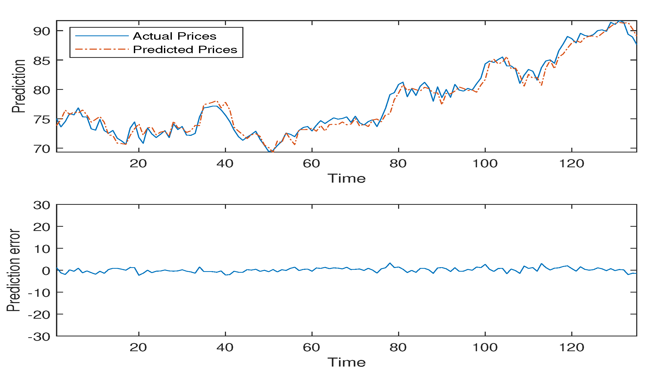
Table 3, Table 4, Table 5 and Table 6 list the results of the four models. Figure 2, Figure 3, Figure 4, Figure 5 and Figure 6 detail the empirical results of the proposed model including: the actual oil prices, predicted values, and model residuals. These figures display the forecasting capabilities of the DMKL models and demonstrate that the proposed model can instantaneously track price fluctuations. As shown by the four tables, DMKL performed the best. FFNN was the second, ARIMA the third, and GRNN performed the worst. The DMKL model significantly outperformed the others and it substantially reduced the forecasting errors. The FFNN, ARIMA and GRNN are all shallow models. They cannot compete with DMKL.
Performance Comparison Using Theil’s U
Theil’s U coefficient indicates how well a forecasting model performs compared with naive no-change extrapolation. It is different from the MSE, RMSE, MAE, and MAPE indices that emphasize only the forecasting errors. As indicated in Theil [40], “Theil’s U will equal 1 if a forecasting technique is essentially no better than using a naive forecast. Theil’s U values less than 1 indicate that a technique is better than using a naive forecast. Hence, a value equal to zero indicates a perfect fit, and consequently, a better model gives a U value close to zero.” The Theil’s U value can be divided into three components including the bias, variance, and covariance. As the names suggest, the bias part accounts for the bias between actual and predicted values, the variance part represents the inequality accounted for by higher/lower variance in the simulated series, and the covariance part is the residual. Table 7 displays the model performance measured by Theil’s U index.
As shown in Table 7, DMKL was approximately one order better than FFNN, ARIMA, and GRNN based on the Theil’s U index. Figure 7 plots the results of Table 7. Table 8 provides the average error of each model. Figure 8, Figure 9, Figure 10, Figure 11 and Figure 12 displays the details of Table 8. As shown in Table 8, according to the performance ranking measured by average errors, DMKL was the best, followed by FFNN, then by ARIMA, and lastly the GRNN. The average RMSE, MAE, and MAPE errors of DMKL were approximately than those of the GRNN, and the reduction was even greater for the MSE.
5. Conclusions
This study focused on developing advanced techniques in oil price forecasting, which is one basis for implementing an effecting hedging or trading strategy. The success of the proposed forecasting model was derived from the combination of multiple kernel machines and deep kernel representation. Deep kernel representation provides a solid foundation for extracting the key features of oil price dynamics. The kernels embedded in a directed acyclic graph provides a deep model that is good at representing complex, compositional, and hierarchical data features. This study used a deep multiple kernel learning for oil price forecasting that eliminated the drawbacks of traditional neural network and support vector machine models. DMKL is successful at high-dimensional data representation and performing non-linear variable selection. By using DMKL, we can both select which variables should enter and the corresponding degrees of interaction complexity. This study applied five major crude oil prices for testing. Empirical results showed that our model was robust, and it systematically outperformed traditional neural networks and regression models. The new model significantly reduced the forecasting errors.
This study developed a highly effective framework for energy commodity price forecasting. The proposed model combines the strengths of kernel methods and deep learning. It can achieve better performance easily. The strength of kernel methods is that they can learn a complex decision boundary with only a few parameters by projecting the data onto a potentially infinite-dimensional reproducing kernel Hilbert space. On the basis of kernel methods and deep learning, the proposed model works by combining multiple kernels within each layer to increase the richness of representations, and by stacking many layers to process a signal in an increasingly abstract manner. Oil price dynamics are complex, nonlinear, and non-stationary. Traditional models tends to be linear, parametric, and shallow, which are not suitable for oil price forecasting. Extracting data features in an abstract manner using a directed acyclic graph (as in our study) is a good strategy to handle complex oil price dynamics.
In summary, the effective framework of this study is also suitable for applications in other forecasting problems. With the leverage of cloud computing, or multiple GPUs on the CUDA (Compute Unified Device Architecture) platform, the system can be applied to online forecasting. Energy commodity investors can also apply the proposed system to effectively hedge their risk in global investments.
Implications and Limitations of This Study, and Suggestions for Future Research
Oil is an important energy commodity, and its price is influenced by many factors, which makes capturing its dynamics quite challenging and leads to difficulties in forecasting. However, with the advances in electronic transactions, vast amounts of financial market data can been collected in real time. Owing to the real time information flow, global markets are closely correlated with instant interactions, especially in the oil and financial markets. This study used information from oil, gold, and currency markets to serve as multiple inputs for our forecasting system. Considering more real time information from global markets is not difficult for future research. However, the computational loading is heavy. Implementing the algorithm in an IC (Interrgrated Circuit) chip is a good solution to achieve the real time response.
There are certain limitations in the study, which may in turn provide fruitful avenues for future studies. First, the DMKL model working in time domains may be not very effective at capturing oil price dynamics. Transforming to a good feature space, such as wavelet domain, could enhance the prediction. However, this would have required more computations, and the loading would be heavier for our algorithm. Second, for simplicity and reducing computation loading, this study employed a global model. The weakness of global models is that they cannot fit each dynamic region very well. However, their strength is that they are easy to implement and are suitable for online applications. Third, this study used data sets of oil, gold, and currency markets only. There are other factors that are also influential in oil prices, such as the supply, demand, GDP, consumer price levels, and commodities markets, and future studies may consider these variables. Fourth, trading is also an important issue for future research. There are many strategies to trading, which poses several issues in finance, for example, price trading, volatility trading, paired trading, and hedge trading, which were beyond the scope of this study. Further investigation is required to determine how to effectively use the forecasting power of this study for trading requirements. Finally, market data that can be collected becomes very large. Complex high-dimensional data tends to obscure the essential feature of data. Identifying intrinsic characteristics and structure of high-dimensional data is important for various fields of research, not limited to the oil price forecasting. Due to the curse of dimensionality, considering sparse modeling (coding) or dimensionality reductions (such as manifold learning) for high-dimensional data will be very important in performance improvements.
Author Contributions
S.-C.H. designed the research and performed the experiments; C.-F.W. collected the data and analyzed the results; S.-C.H. wrote the paper; C.-F.W. edited the paper.
Funding
This research was funded by the Ministry of Science and Technology, Taiwan (MOST 107-2410-H-018-004).
Acknowledgments
The authors would like to thank the anonymous reviewers for their valuable comments and suggestions which contributed to the improvement of this study.
Conflicts of Interest
The authors declare no conflict of interest.
References
- Abosedra, S.; Baghestani, H. On the predictive accuracy of crude oil future prices. Energy Policy 2004, 32, 1389–1393. [Google Scholar] [CrossRef]
- Atsalakis, G.; Valavanis, K. Surveying stock market forecasting techniques—Part II: Soft computing methods. Expert Syst. Appl. 2009, 36, 5932–5941. [Google Scholar] [CrossRef]
- Atsalakis, G.; Valavanis, K. Surveying Stock Market Forecasting Techniques—Part I: Conventional Methods. J. Comput. Optim. Econ. Financ. 2010, 2, 4. [Google Scholar]
- Fan, L.; Li, H. Volatility analysis and forecasting models of crude oil prices: A review. Int. J. Glob. Energy Issues 2015, 38, 5–17. [Google Scholar] [CrossRef]
- Bahrammirzaee, A. A comparative survey of artificial intelligence applications in finance: Artificial neural networks, expert system and hybrid intelligent systems. Neural Comput. Appl. 2010, 19, 1165–1195. [Google Scholar] [CrossRef]
- Krollner, B.; Vanstone, B.; Finnie, G. Financial time series forecasting with machine learning techniques: A survey. In Proceedings of the 8th European Symposium on Artificial Neural Networks, Bruges, Belgium, 28–30 April 2010. [Google Scholar]
- Gupta, R.; Wohar, M. Forecasting oil and stock returns with a Qual VAR using over 150 years off data. Energy Econ. 2017, 62, 181–186. [Google Scholar] [CrossRef] [Green Version]
- Gavriilidis, K.; Kambouroudis, D.S.; Tsakou, K.; Tsouknidis, D.A. Volatility forecasting across tanker freight rates: The role of oil price shocks. Transp. Res. Part E Logist. Transp. Rev. 2018, 118, 376–391. [Google Scholar] [CrossRef]
- Herrera, A.M.; Hu, L.; Pastor, D. Forecasting crude oil price volatility. Int. J. Forecast. 2018, 34, 622–635. [Google Scholar] [CrossRef]
- Morana, C. A semiparametric approach to short–term oil price forecasting. Energy Econ. 2010, 23, 325–338. [Google Scholar] [CrossRef]
- Ding, Y. A novel decompose-ensemble methodology with AIC-ANN approach for crude oil forecasting. Energy 2018, 154, 328–336. [Google Scholar] [CrossRef]
- Yu, L.; Wang, S.; Lai, K.K. Forecasting crude oil price with an EMD-based neural network ensemble learning paradigm. Energy Econ. 2008, 30, 2623–2635. [Google Scholar] [CrossRef]
- Naderi, M.; Khamehchi, E.; Karimi, B. Novel statistical forecasting models for crude oil price, gas price, and interest rate based on meta–heuristic bat algorithm. J. Pet. Sci. Eng. 2019, 172, 13–22. [Google Scholar] [CrossRef]
- Safari, A.; Davallou, M. Oil price forecasting using a hybrid model. Energy 2018, 148, 49–58. [Google Scholar] [CrossRef]
- Li, T.; Zhou, M.; Guo, C.; Luo, M.; Wu, J.; Pan, F.; Tao, Q.; He, T. Forecasting Crude Oil Price Using EEMD and RVM with Adaptive PSO–Based Kernels. Energies 2016, 9, 1014. [Google Scholar] [CrossRef]
- Wang, Q.; Li, S.; Li, R. China’s dependency on foreign oil will exceed 80% by 2030: Developing a novel NMGM-ARIMA to forecast China’s foreign oil dependence from two dimensions. Energy 2018, 163, 151–167. [Google Scholar] [CrossRef]
- Xiao, J.; Li, Y.; Xie, L.; Liu, D.; Huang, J. A hybrid model based on selective ensemble for energy consumption forecasting in China. Energy 2018, 159, 534–546. [Google Scholar] [CrossRef]
- Drachal, K. Determining Time-Varying Drivers of Spot Oil Price in a Dynamic Model Averaging Framework. Energies 2018, 11, 1207. [Google Scholar] [CrossRef]
- Iranmanesh, H.; Abdollahzade, M.; Miranian, A. Mid-Term Energy Demand Forecasting by Hybrid Neuro-Fuzzy Models. Energies 2012, 5, 1–21. [Google Scholar] [CrossRef]
- Vapnik, V. The Nature of Statistical Learning Theory; Springer Science & Business Media: Berlin, Germany, 2013. [Google Scholar]
- Schoelkopf, B.; Burges, C.J.C.; Smola, A.J. Advances in kernel Methods—Support Vector Learning; MIT Press: Cambridge, MA, USA, 1999. [Google Scholar]
- Ding, Z.J.; Min, Q.; Lin, Y. Application of ARIMA model in forecasting prude oil price. Logist. Technol. 2008, 27, 156–159. [Google Scholar]
- Khashman, A.; Nwulu, N.I. Support vector machines versus back propagation algorithm for oil price prediction. In Proceedings of the 8th International Conference on Advances in Neural Networks, Guilin, China, 29 May–1 June 2011. [Google Scholar]
- Liu, J.P.; Lin, S.; Guo, T.; Chen, H.Y. Nonlinear time series forecasting model and its application for oil price forecasting. J. Manag. Sci. 2011, 24, 104–112. [Google Scholar]
- Wang, Q.; Li, S.; Li, R. Forecasting energy demand in China and India: Using single-linear, hybrid-linear, and non-linear time series forecast techniques. Energy 2018, 161, 821–831. [Google Scholar] [CrossRef]
- Xie, W.; Yu, L.; Xu, S.; Wang, S. A new method for crude oil price forecasting based on support vector machines. Lect. Notes Comput. Sci. 2006, 3994, 444–451. [Google Scholar]
- Lanckriet, G.R.G.; Cristianini, N.; Ghaoui, L.E.; Bartlett, P.; Jordan, M.I. Learning the kernel matrix with semidefinite programming. J. Mach. Learn. Res. 2004, 5, 27–72. [Google Scholar]
- Bach, F. Exploring Large Feature Spaces with Hierarchical Multiple Kernel Learning. In Advances in Neural Information Processing Systems (NIPS); Curran Associates: New York, NY, USA, 2008. [Google Scholar]
- Bach, F. High–Dimensional Non–Linear Variable Selection through Hierarchical Kernel Learning. arXiv, 2009; arXiv:0909.0844. [Google Scholar]
- Bengio, Y.; LeCun, Y.; Hinton, G. Deep Learning. Nature 2015, 521, 436–444. [Google Scholar]
- Schmidhuber, J. Deep Learning in Neural Networks: An Overview. Neural Netw. 2015, 61, 85–117. [Google Scholar] [CrossRef] [PubMed]
- He, K.; Zhang, X.; Ren, S.; Sun, J. Deep residual learning for image recognition. arXiv, 2016; arXiv:1512.03385. [Google Scholar]
- Ioffe, S.; Szegedy, C. Batch normalization: Accelerating deep network training by reducing internal covariate shift. arXiv, 2015; arXiv:1502.03167. [Google Scholar]
- Krizhevsky, A.; Sutskever, I.; Hinton, G.E. Imagenet classification with deep convolutional neural networks. In Proceedings of the 25th International Conference on Neural Information Processing Systems, Lake Tahoe, NV, USA, 3–6 December 2012. [Google Scholar]
- Simonyan, K.; Zisserman, A. Very deep convolutional networks for large-scale image recognition. In Proceedings of the International Conference on Learning Representations 2015, San Diego, CA, USA, 7–9 May 2015. [Google Scholar]
- Huang, C.L.; Wang, C.J. A GA-based feature selection and parameters optimization for support vector machines. Expert Syst. Appl. 2006, 31, 231–240. [Google Scholar] [CrossRef]
- Ren, Y.; Bai, G. Determination of Optimal SVM Parameters by Using GA/PSO. J. Comput. 2010, 5, 1160–1168. [Google Scholar] [CrossRef]
- Bellman, R.E. Adaptive Control Processes: A Guided Tour; Princeton University Press: Princeton, NJ, USA, 2015; Volume 2045. [Google Scholar]
- Drezet, P.M.L.; Harrison, R.F. Support vector machines for system identification. In Proceedings of the UKACC International Conference on Control 1998, Swansea, UK, 1–4 September 1998; pp. 688–692. [Google Scholar]
- Theil, H. Applied Economic Forecasting; North Holland: Amsterdam, The Netherlands, 1966. [Google Scholar]
Figure 1.
Flow diagram of the proposed system.

Figure 2.
The proposed model forecasts on WTI crude oil prices.

Figure 3.
The proposed model forecasts on Brent crude oil prices.

Figure 4.
The proposed model forecasts on Forties crude oil prices.

Figure 5.
The proposed model forecasts on Dubai crude oil prices.

Figure 6.
The proposed model forecasts on Oman crude oil prices.

Figure 7.
Performance comparison of the Theil’s U index.

Figure 8.
Performance comparison of the average RMSE index.

Figure 9.
Performance comparison of the average MSE index.

Figure 10.
Performance comparison of the average MAE index.

Figure 11.
Performance comparison of the average MAPE index.

Figure 12.
Performance comparison of the average Theil’s U index.


Table 1.
Descriptive statistics of each variable.
| Brent | WTI | Dubai | Oman | Forties | Gold | US/TWD | |
|---|---|---|---|---|---|---|---|
| mean | 74.07 | 74.00 | 72.58 | 72.88 | 73.63 | 937.56 | 32.59 |
| min | 45.97 | 45.82 | 44.19 | 46.34 | 45.32 | 704.90 | 31.04 |
| max | 94.55 | 91.48 | 91.28 | 91.71 | 93.72 | 1217.40 | 35.17 |
| standard deviation | 9.78 | 9.35 | 9.44 | 9.13 | 9.71 | 109.15 | 0.80 |
| median | 75.67 | 75.20 | 74.17 | 73.62 | 75.10 | 926.90 | 32.35 |
| skewness | −0.71 | −0.94 | −0.97 | −0.92 | −0.73 | 0.29 | 1.01 |
| kurtosis | 3.57 | 3.80 | 4.13 | 4.14 | 3.57 | 2.66 | 3.77 |
Table 2.
The p-values of unit root tests.
| 0 | 1 | 2 | |
|---|---|---|---|
| Brent | 0.1527 | 0.1426 | 0.1248 |
| WTI | 0.1980 | 0.1385 | 0.1490 |
| Dubai | 0.1496 | 0.1644 | 0.1595 |
| Oman | 0.1707 | 0.2160 | 0.1832 |
| Forties | 0.1406 | 0.1389 | 0.1219 |
| Gold | 0.2835 | 0.1887 | 0.2114 |
| US/TWD | 0.4931 | 0.4318 | 0.5146 |
Table 3.
Performance of the DMKL model on major oil prices.
| WTI | Brent | Forties | Dubai | Oman | |
|---|---|---|---|---|---|
| RMSE | 1.4934 | 1.4021 | 1.4677 | 1.5039 | 1.0440 |
| MSE | 2.2303 | 1.9658 | 2.1541 | 2.2616 | 1.0899 |
| MAE | 1.1966 | 1.1261 | 1.1840 | 1.2151 | 0.8391 |
| MAPE | 0.0150 | 0.0139 | 0.0148 | 0.0155 | 0.0107 |
Table 4.
Performance of the ARIMA model on major oil prices.
| WTI | Brent | Forties | Dubai | Oman | |
|---|---|---|---|---|---|
| RMSE | 4.1014 | 4.147 | 4.9432 | 3.9687 | 3.9804 |
| MSE | 16.8219 | 17.1979 | 24.4353 | 15.7504 | 15.8436 |
| MAE | 3.464 | 3.1505 | 3.8171 | 3.4091 | 3.3208 |
| MAPE | 0.0425 | 0.0373 | 0.0453 | 0.0445 | 0.0431 |
Table 5.
Performance of the GRNN model on major oil prices.
| WTI | Brent | Forties | Dubai | Oman | |
|---|---|---|---|---|---|
| RMSE | 4.7763 | 5.1177 | 5.0444 | 5.1320 | 5.6525 |
| MSE | 22.8131 | 26.1906 | 25.4463 | 26.3375 | 31.9504 |
| MAE | 3.9415 | 4.1265 | 4.0792 | 4.2214 | 4.6962 |
| MAPE | 0.0479 | 0.0487 | 0.0487 | 0.0519 | 0.0582 |
Table 6.
Performance of the FFNN model on major oil prices.
| WTI | Brent | Forties | Dubai | Oman | |
|---|---|---|---|---|---|
| RMSE | 2.2592 | 1.7016 | 2.1841 | 2.0506 | 2.2834 |
| MSE | 5.1041 | 2.8953 | 4.7703 | 4.2050 | 5.2140 |
| MAE | 1.8509 | 1.4178 | 1.7825 | 1.5793 | 1.9936 |
| MAPE | 0.0229 | 0.0175 | 0.0216 | 0.0195 | 0.0262 |
Table 7.
Performance comparison of the Theil’s U index.
| WTI | Brent | Forties | Dubai | Oman | |
|---|---|---|---|---|---|
| DMKL | 0.0093 | 0.0086 | 0.0091 | 0.0095 | 0.0067 |
| FFNN | 0.0141 | 0.0104 | 0.0136 | 0.0130 | 0.0144 |
| GRNN | 0.0302 | 0.0319 | 0.0317 | 0.0330 | 0.0366 |
| ARIMA | 0.0259 | 0.0257 | 0.0311 | 0.0248 | 0.0252 |
Table 8.
Average error of each model.
| DMKL | FFNN | GRNN | ARIMA | |
|---|---|---|---|---|
| RMSE | 1.38222 | 2.09578 | 5.14458 | 4.22814 |
| MSE | 1.94034 | 4.43774 | 26.54758 | 18.00982 |
| MAE | 1.11218 | 1.72482 | 4.21296 | 3.43230 |
| MAPE | 0.01398 | 0.02154 | 0.05108 | 0.04254 |
| Theil’s U | 0.00864 | 0.01310 | 0.03268 | 0.02654 |
© 2018 by the authors. Licensee MDPI, Basel, Switzerland. This article is an open access article distributed under the terms and conditions of the Creative Commons Attribution (CC BY) license (http://creativecommons.org/licenses/by/4.0/).
Share and Cite
MDPI and ACS Style
Huang, S.-C.; Wu, C.-F. Energy Commodity Price Forecasting with Deep Multiple Kernel Learning. Energies 2018, 11, 3029. https://doi.org/10.3390/en11113029
AMA Style
Huang S-C, Wu C-F. Energy Commodity Price Forecasting with Deep Multiple Kernel Learning. Energies. 2018; 11(11):3029. https://doi.org/10.3390/en11113029
Chicago/Turabian StyleHuang, Shian-Chang, and Cheng-Feng Wu. 2018. "Energy Commodity Price Forecasting with Deep Multiple Kernel Learning" Energies 11, no. 11: 3029. https://doi.org/10.3390/en11113029
Note that from the first issue of 2016, this journal uses article numbers instead of page numbers. See further details here.