Abstract
The smart building concept aims to use smart technology to reduce energy consumption, as well as to improve comfort conditions and users’ satisfaction. It is based on the use of smart sensors and software to follow both outdoor and indoor conditions for the control of comfort, and security devices for the optimization of energy consumption. This paper presents a data-based model for indoor temperature forecasting, which could be used for the optimization of energy device use. The model is based on an artificial neural network (ANN), which is validated on data recorded in an old building. The novelty of this work consists of the methodology proposed for the development of a simplified model for indoor temperature forecasting. This methodology is based on the selection of pertinent input parameters after a relevance analysis of a large set of input parameters, including solar radiation outdoor temperature history, outdoor humidity, indoor facade temperature, and humidity. It shows that an ANN-based model using outdoor and facade temperature sensors provides good forecasting of indoor temperatures. This model can be easily used in the optimal regulation of buildings’ energy devices.
1. Introduction
The smart building concept aims to use smart technology to reduce energy consumption, as well as to improve comfort and users’ satisfaction. Forecasting of the indoor temperature is necessary for the regulation of energy devices to ensure occupant comfort, as well as for energy optimization [1,2]. This forecasting constitutes a complex task, because it is governed by complex physical and behavioral phenomena. It is affected by a multitude of parameters, which could be classified into three groups: outdoor conditions, building characteristics, and occupants’ behavior [3,4,5]. In addition, investigations showed that the indoor temperature does not have uniform distribution [6].
Indoor temperature forecasting could be carried out using physical or data-driven approaches [7]. The physical approach is based on the use of numerical modelling [8,9], which requires detailed information about a building’s characteristics, appliances, and occupant behavior.
The data-driven approach is based on the use of collected data for developing relationships (models) between ‘input’ parameters and ‘output’ parameters. These relationships could be established by learning from collected data. The artificial neural network (ANN) approach was used to build data-driven models [10,11,12]. Soleimani-Mohseni et al. [13] showed that the operative temperature could be well estimated by the ANN approach using the indoor air temperature, electrical power, outdoor temperature, time of day, wall temperature, and ventilation flow rate. Lu and Viljanen [14] used the ANN approach to predict air temperature and relative humidity in a test room using indoor and outdoor temperature and humidity. Recently, Zabada and Shahrour [15] used the ANN approach for the analysis of the heating expenses in social housing. In these works, the ANN model was used as a prediction tool for specific cases. This paper proposes a methodology, which could be followed for the use of the ANN approach for the indoor temperature forecasting in any type of building. This methodology is based on the use of a relevance analysis for the determination of pertinent input parameters and the optimal ANN architecture. The methodology is presented through its application on data recorded in an old building.
2. Data Collection
Data were collected using a smart monitoring of an old building of Polytech’Lille Engineering School in the north of France. Monitoring concerned indoor and outdoor temperature and humidity, as well as solar radiation [16,17]. Parameters were recorded at five-minute intervals and then sent to a local server. Figure 1 illustrates an example of recorded data on a summer day. Data concerns the outdoor temperature, as well as the indoor temperature at three locations in the office: facade, center of the lateral wall, and office center. The external temperature varied between 17.5 °C and 34 °C, while the facade indoor temperature varied between 21 °C and 25.5 °C. The temperatures at the center of the office and the center of the lateral wall varied between 22 °C and 24.2 °C.
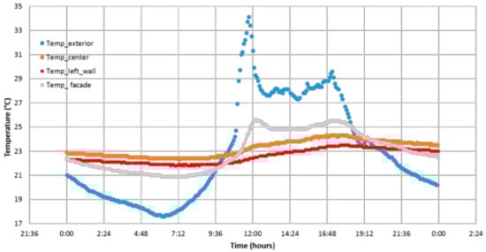
Figure 1.
Temperature variation on a summer day.
Data were collected for two summer months (June and July) in different offices of the building.
3. Artificial Neural Network Approach
The ANN approach is inspired from the ability of the human brain to predict patterns based on learning and recalling processes. It allows the construction of relationships between input parameters and output parameters using artificial neurons, which are arranged in an input layer, an output layer and one or more hidden layers [18]. Analyses were conducted using the multilayer back-propagation neural network. We used a three-layer ANN with n, m, and k as the number of input, hidden, and output nodes, respectively, based on the equation:
where stands for the output values and denotes the input values; gives the weights of connection between the input layer and the hidden layer.
The ANN performances could be evaluated using the mean square error (MSE) and the coefficient of correlation (R)
where ei is the error between the ANN output (Yi) and the experimental input (Xi), represents the mean of the input target.
Different ANN architectures exist. The multilayer perception (MLP) structure is the most popular [19,20,21,22,23,24]. Its use with a single hidden layer and a sufficient number of neurons provided good accuracy for the approximated function [25,26]. This architecture is used in this work.
The use of ANN for temperature forecasting aims to predict the building indoor temperature for the optimal regulation of energy devices as well as for ensuring occupants’ comfort. Indoor conditions of a building are highly affected by its age and thermal performance, which depends on its envelope and construction material. The input parameters concern the outdoor conditions, indoor conditions, as well as the occupants’ behavior. The forecasting time depends on the building thermal inertia and energy regulation system. Each building is characterized by its time lag and the time of heat transmission delay [27,28,29,30]. The prediction time for ANN models ranged from 0.5 to 4 h to cover the phase of heating exchange through the facade and to investigate the effectiveness of this approach.
This paper proposes a methodology composed of two steps for the use of the ANN approach for indoor temperature forecasting. The first step concerns the indoor facade temperature forecasting considering outdoor and indoor conditions, while the second step concerns the prediction of the temperature at the room center considering the indoor facade temperature.
Analyses were conducted using MATLAB (Mathworks Inc., Natick, MA, USA—Group License) for ANN modeling and IBM SPSS statistics for input parameter ranking.
4. Facade Indoor Temperature Forecasting
4.1. Analysis of the Input Parameters’ Relevance
The input parameters used in the global analysis are summarized in Table 1. They concern the outdoor conditions (temperature, humidity, and solar radiation), outdoor temperature history (input matrix for the last 3-h values having 30 min lag between its different columns: if the actual outdoor temperature was recorded at time t, the history matrix corresponds to t—0.5 h, t—1 h, t—1.5 h, t—2 h, t—2.5 h, and t—3 h, the indoor facade temperature history (similar matrix history as the outdoor temperature), and time (cumulative minutes of the day). The time range of history inputs was chosen with respect to the prediction time to cover the phase shift that will occur at the facade level. The impact of a larger range (t—5 h, t—6 h, etc.) for the history inputs did not affect the results. A 30 min lag was chosen to detect any sudden variation at the facade level.

Table 1.
Input parameters for the facade temperature forecasting.
The ANN optimal architecture (Figure 2) was fixed after several comparative analyses. It includes one hidden layer with four neurons. Table 2 provides the weights of neurons’ connections obtained from MATLAB software. We can observe that the weight could be negative or positive providing excitatory or inhibitory influence on each input.
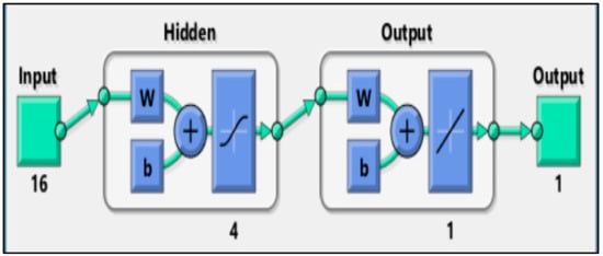
Figure 2.
Artificial Neural Network (ANN) optimal architecture.
Table 2.
Weight of neurons’ connections.
Figure 3 shows comparison of ‘predicted’ and ‘recorded’ facade temperatures. We observe a good agreement between these values with R = 0.9967 and MSE = 0.0277. This result shows that the ANN model predicts well the facade indoor temperature. The determination of input parameters requires two temperature sensors (outdoor and indoor), an external humidity sensor, and a solar radiation sensor.
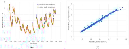
Figure 3.
Predicted and recorded facade temperatures: (a) variation of both temperatures in time domain; and (b) the predicted facade temperature with the recorded facade temperature.
In order to determine the most important input parameters in the ANN model, IBM SPSS statistical software was used to analyze the ‘importance’ of these parameters. This software is based on inferential statistics. It uses recorded data to perform a sensitivity analysis for the determination of the importance of each input parameter. Table 3 summarizes the obtained results. It shows that the solar radiation, time and humidity have a low role in the forecasting model, with an importance factor lower than 5.1%. The outdoor temperature has the highest importance (Importance Factor = 42%), followed by the historical facade temperature (Importance Factor = 31.9%). The historical outdoor temperature has an intermediate influence with an Importance Factor = 12.8%.
Table 3.
Analysis of the relevance of input parameters.
Since the role of some input parameters in the ANN model is very weak (with reference to the SPSS classification), analyses were conducted by neglecting these parameters. Table 4 summarizes the results of these analyses. It shows clearly that the neglect of solar radiation, humidity, and historical outdoor temperature (Model 5) does not significantly deteriorate the quality of the ANN model: the mean square error (MSE) increases from 0.0277 to 0.0365, while the coefficient of correlation (R) decreases from 0.9967 to 0.9959. The additional neglect of the historical data of the facade temperature (Model 6) has a higher influence: MSE increases from 0.0277 to 0.4922, while R decreases from 0.9967 to 0.946. Figure 4 illustrates the results of Models 1, 5, and 6. As expected and according to the physics of the heat transfer in transient conditions, this result shows that the facade temperature could be effectively predicted in considering only the outdoor temperature and the historical data of the facade indoor temperature.
Table 4.
Degraded model results.
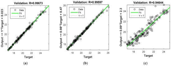
Figure 4.
R results for different models: (a) Model 1; (b) Model 5; and (c) Model 6.
4.2. Facade Temperature Forecasting Model
4.2.1. Use of the Outdoor Temperature as Input Parameter
Considering the results of the previous section, the outdoor temperature is first used as the input parameter for forecasting the facade indoor temperature. The forecasting model provides the temperature at 0.5, 1, 2, and 4 h.
Figure 5 and Figure 6 show the forecasting results at 0.5 and 1.0 h. We observe that the ANN model reproduces well the recorded temperature. For 0.5-h forecasting, R is equal to 0.956 and MSE is equal to 0.4369; while for one-hour forecasting, R = 0.928 and MSE = 0.48454. Figure 7 shows the forecasting error distribution for 0.5 and one hour. It shows that about 90% of the forecasting error are less than 1 °C.
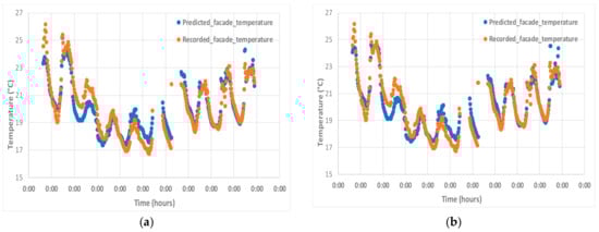
Figure 5.
Recorded and predicted facade temperature variation in the time domain: (a) prediction for 0.5 h; and (b) prediction for 1 h.
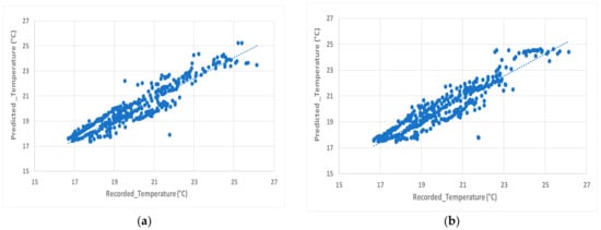
Figure 6.
Predicted facade temperature with the recorded facade temperature (input parameter = outdoor temperature): (a) prediction for 0.5 h; and (b) prediction for 1 h.
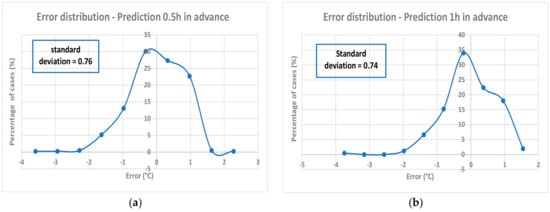
Figure 7.
Distribution of the error forecasting (input parameter = outdoor temperature): (a) prediction for 0.5 h; and (b) prediction for 1 h.
Figure 8 and Figure 9 shows the forecasting results at two and four hours. We observe a deterioration in the quality of forecasting regarding those obtained at 0.5 and one hour. For two-hour forecasting, R = 0.9109 and MSE = 0.89078, while for four-hour forecasting, R = 0.8370 and MSE = 1.23783. Figure 10 shows the forecasting error distribution for two and four hours. It shows that for the former, about 70% of the forecasting error are less than 1 °C, while for the latter about 64% of the forecasting error are less than 1 °C. Table 5 summarizes the forecasting results.
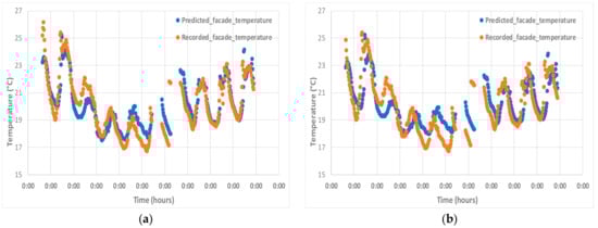
Figure 8.
Recorded and predicted facade temperature variation in the time domain: (a) prediction for 2 h; (b) prediction for 4 h.
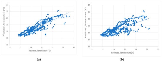
Figure 9.
Predicted facade temperature with the recorded facade temperature (input parameter = outdoor temperature): (a) prediction for 2 h; and (b) prediction for 4 h.
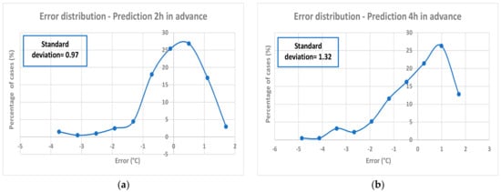
Figure 10.
Distribution of error forecasting (input parameter = outdoor temperature): (a) prediction for 2 h; and (b) prediction for 4 h.
Table 5.
Performances of the forecasting models (input parameter = outdoor temperature)
4.2.2. Use of the Outdoor Temperature and the History of the Facade Temperature as Input Parameters
In this section, both outdoor temperature and three-hour facade temperature history are used as input parameters in the forecasting model. The forecasting model provides the temperature at 0.5, 1, 2, and 4 h. Table 6 summarizes the obtained results. The temperature forecasting is improved regarding the forecasting model using the outdoor temperature as input. This result is particularly interesting for the temperature foresting at two hours: R = 0.957 and MSE = 0.3299 to be compared with R = 0.9109 and MSE = 0.89078 obtained with the outdoor temperature as input parameter. Figure 11 shows the forecasting error distribution for two hours. It shows that about 88% of the forecasting error are less than 1 °C to be compared with 70% obtained with the previous model.
Table 6.
Performances of the forecasting models (input parameters = outdoor temperature and three-hour facade temperature)
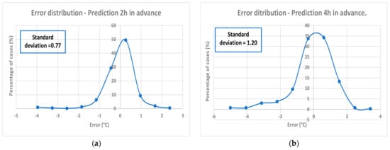
Figure 11.
Distribution of error forecasting (input parameter = outdoor temperature and 3-h facade temperature): (a) prediction for 2 h; and (b) prediction for 4 h.
The four-hour foresting is still weak with R = 0.852; MSE = 1.0533. About 68% of the forecasting error are less than 1 °C (Figure 11).
4.3. Indoor Temperature Forecasting (Room Center)
The ANN approach is used for forecasting the temperature at the room center considering only the facade temperature as input parameter. Figure 12 shows a comparison of ‘predicted’ and ‘recorded’ indoor temperatures. A good agreement is observed between recorded temperature and ANN prediction with R = 0.951; MSE = 0.1679. Only 1% of data has an error greater than 1 °C (Figure 13).
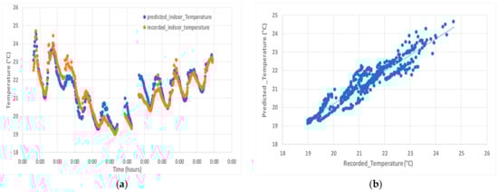
Figure 12.
Predicted and recorded indoor temperatures: (a) the variation of both temperatures in time domain; and (b) the predicted indoor temperature with the recorded indoor temperature.
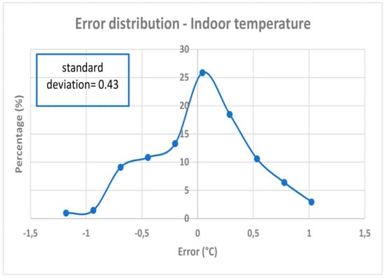
Figure 13.
Distribution of error forecasting for indoor temperature (input parameters = facade temperature).
5. Discussion of Results
Relevance analysis and ANN modeling using different sets of input parameters showed that the indoor temperature forecasting could be conducted with good precision considering only outdoor temperature and indoor facade temperature history. Indeed, the influence of solar radiation, humidity, and outdoor temperature history in the forecasting model could be neglected. The prediction of the facade temperature was conducted with different inputs parameters and for different forecasting times. In the example presented in this paper, predictions were good up to two hours. The four-hour prediction gave unsatisfactory results with R = 0.852; MSE = 1.0533.
Indoor temperature forecasting was successfully conducted using the facade temperature. Available data did not include indoor activities. The presence of significant indoor activities—such as meetings, use of energy consuming devices, as well as opening doors and windows—could significantly affect the energy balance in the room. If these activities are significant, they should be monitored and included in the forecasting model.
6. Conclusions
This paper proposed a methodology for the development of a simplified ANN-based model for forecasting indoor temperature. The methodology includes two steps. The first step concerns the forecasting of the indoor facade temperature considering outdoor and indoor conditions, while the second step concerns the prediction of the temperature at the room center considering only the indoor facade temperature.
This paper shows that both relevance analysis and the use of different sets of input parameters could lead to a simplified forecasting model with restricted input parameters. This methodology was illustrated through its application to data collected in an old building. Data included outdoor and indoor temperature and humidity, as well as solar radiation. Analyses showed that two-hour facade temperature forecasting could be conducted with good precision using only the outdoor temperature and three-hour facade temperature history. This result could not be generalized. However, the proposed methodology could be used for other situations by using first only temperature sensors for measuring the outdoor and the indoor facade temperatures. Concerning the second step, the ANN model gave good forecasting of the temperature at the room center in considering only the facade temperature. Available data did not include indoor activities. The presence of significant indoor activities should be considered in the forecasting model.
Acknowledgments
This research received funding by the University of Lille, the French University Agency (AUF) and the Lebanese National Council for Scientific Research CNRS-L.
Author Contributions
Nivine Attoue and Isam Shahrour conceived and designed the experiments; Nivine Attoue performed the experiments; Nivine Attoue, Isam Shahrour and Rafic Younes analyzed the data; Nivine Attoue and Isam Shahrour wrote the paper.
Conflicts of Interest
The authors declare no conflict of interest.
References
- Holz, R.; Hourigan, A.; Sloop, R.; Monkman, P.; Krarti, M. Effects of standard energy conserving measures on thermal comfort. Build. Environ. 1997, 32, 31–43. [Google Scholar] [CrossRef]
- Tham, K.W.; Ullah, M.B. Building energy performance and thermal comfort in Singapore. ASHRAE Trans. 1993, 99, 308–321. [Google Scholar]
- Huebner, G.M.; McMichael, M.; Shipworth, D.; Shipworth, M.; Durand-Daubin, M.; Summerfield, A. The reality of English living rooms, a comparison of internal temperatures against common model assumptions. Energy Build. 2013, 66, 688–696. [Google Scholar] [CrossRef]
- Nguyen, J.L.; Schwartz, J.; Dockery, D.W. The relationship between indoor and outdoor temperature, apparent temperature, relative humidity and absolute humidity. Indoor Air 2014, 24, 103–112. [Google Scholar] [CrossRef] [PubMed]
- Hens, H.; Parijs, W.; Deurinck, M. Energy consumption for heating and rebound effects. Energy Build. 2010, 42, 105–110. [Google Scholar] [CrossRef]
- Shao, X.; Ma, X.; Li, X.; Liang, C. Fast prediction of non-uniform temperature distribution: A concise expression and reliability analysis. Energy Build. 2017, 141, 295–307. [Google Scholar] [CrossRef]
- Ruano, A.E.; Crispim, E.M.; Conceição, E.Z.E.; Lucio, M.M.J.R. Prediction of building’s temperature using neural networks models. Energy Build. 2006, 38, 682–694. [Google Scholar] [CrossRef]
- Fang, P.; Liu, T.; Liu, K.; Zhang, Y.; Zhao, J. A Simulation model to calculate temperature distribution of an air-conditioned room. In Proceedings of the 2016 8th International Conference on Intelligent Human-Machine Systems and Cybernetics, Hangzhou, China, 27–28 August 2006. [Google Scholar]
- Jigang, Z. Study on the Airflow & Temperature Field Characteristics in the Room with Wall Air Conditioner and on the Human Thermal Comfort; Shandong University: Jinan, China, 2007. [Google Scholar]
- Funahashi, K. On the approximate realization of continuous mappings by neural networks. Neural Netw. 1989, 2, 183–192. [Google Scholar] [CrossRef]
- Hornik, K.; Stinchcombe, M.; White, H. Multilayer feed forward networks are universal approximators. Neural Netw. 1989, 2, 359–366. [Google Scholar] [CrossRef]
- Girosi, F.; Poggio, T. Networks and the Best Approximation Property. Biol. Cybern. 1990, 63, 169–176. [Google Scholar] [CrossRef]
- Soleimani-Mohseni, M.; Thomas, B.; Fahlén, P. Estimation of operative temperature in buildings using artificial neural network. Energy Build. 2006, 38, 635–640. [Google Scholar] [CrossRef]
- Lu, T.; Viljanen, M. Prediction of indoor temperature and relative humidity using neural network models: Model comparison. Neural Comput. Appl. 2009, 18, 345–357. [Google Scholar] [CrossRef]
- Zabada, S.; Shahrour, I. Analysis of Heating Expenses in a Large Social Housing Stock Using Artificial Neural Networks. Energies 2017, 10, 2086. [Google Scholar] [CrossRef]
- Aljer, A.; Loriot, M.; Shahrour, I.; Benyahya, A. Smart system for social housing monitoring. In Proceedings of the 2017 Sensors Networks Smart and Emerging Technologies (SENSET), Beirut, Lebanon, 12–14 September 2017; IEEE: Piscataway, NJ, USA, 2017. [Google Scholar] [CrossRef]
- Attoue, N.; Shahrour, I.; Younes, R.; Aljer, A.; Loriot, M. Analysis of Buildings Energy Losses Using Smart Monitoring. In Proceedings of the International Work-Conference on Time Series (ITISE 2017), Granada, Spain, 18–20 September 2017; ISBN 978-84-17293-01-7. [Google Scholar]
- Khayatian, F.; Sarto, L.; Dall’O, G. Application of neural networks for evaluating energy performance certificates of residential buildings. Energy Build. 2016, 125, 45–54. [Google Scholar] [CrossRef]
- Mba, L. Modélisation du Comportement Thermique du Bâtiment: Application d’une Méthode Neuronale; Université de Douala-Cameroun: Douala, Cameroon, 2009. [Google Scholar]
- Mba, L.; Kemajou, A.; Meukam, P. Application of artificial neural network for modeling the thermal behavior of building in humid region. Presented at the Actes des 3ème Rencontres EG@, Yaoundé, Cameroun, 14–16 Septembre 2010. [Google Scholar]
- Brano, V.L.; Ciulla, G.; Falco, M.D. Artificial neural networks to predict the power output of PV panel. Int. J. Photoenergy 2014, 2014, 193083. [Google Scholar] [CrossRef]
- Kemajou, A.; Mba, L.; Meukam, P. Application of artificial neural network for predicting the indoor air temperature in modern building in humid region. Br. J. Appl. Sci. Technol. 2012, 2, 23–34. [Google Scholar] [CrossRef]
- Manssouri, T.; Sahbi, H.; Manssouri, I.; Boudad, B. Utilisation d’un modèle hybride base sur la rlms et les rna-pmc pour la prédiction des paramètres indicateurs de la qualité des eaux souterraines cas de la nappe de Souss-Massa-Maroc. Eur. Sci. J. 2015, 11, 35–46. [Google Scholar]
- Paudel, S.; Elmtiri, M.; Kling, W.L.; Le Corre, O.; Lacarrière, B. Pseudo dynamic transitional modeling of building heating energy demand using artificial neural network. Energy Build. 2014, 70, 81–93. [Google Scholar] [CrossRef]
- Tasadduq, I.; Rehman, S.; Bubshait, K. Application of neural networks for the prediction of hourly mean surface temperatures in Saudi Arabia. Renew. Energy 2002, 25, 545–554. [Google Scholar] [CrossRef]
- Said, S.M. Degree-day base temperature for residential building energy prediction in Saudia Arabia. ASHRAE Trans. 1992, 98, 346–353. [Google Scholar]
- Ding, Y.; Zhang, Q.; Yuan, T.; Yang, K. Model input selection for building heating load prediction: A case study for an office building in Tianjin. Energy Build. 2018, 159, 254–270. [Google Scholar] [CrossRef]
- Ferrari, S. Building envelope and heat capacity: Re-discovering the thermal mass of winter energy savings. In Proceedings of the 28th AIVC Conference, Crete, Greece, 27–29 September 2007. [Google Scholar]
- Gagliano, A.; Patania, F.; Nocera, F.; Signorello, C. Assessment of the dynamic thermal performance of massive buildings. Energy Build. 2014, 72, 361–370. [Google Scholar] [CrossRef]
- Ulgen, K. Experimental and theoretical investigation of effects of walls’ thermos-physical properties on time lag and decrement factor. Energy Build. 2002, 34, 273–278. [Google Scholar] [CrossRef]
© 2018 by the authors. Licensee MDPI, Basel, Switzerland. This article is an open access article distributed under the terms and conditions of the Creative Commons Attribution (CC BY) license (http://creativecommons.org/licenses/by/4.0/).