Modelling the Effect of Driving Events on Electrical Vehicle Energy Consumption Using Inertial Sensors in Smartphones

Abstract

Air pollution and climate change are some of the main problems that humankind is currently facing. The electrification of the transport sector will help to reduce these problems, but one of the major barriers for the massive adoption of electric vehicles is their limited range. The energy consumption in these vehicles is affected, among other variables, by the driving behavior, making range a value that must be personalized to each driver and each type of electric vehicle. In this paper we offer a way to estimate a personalized energy consumption model by the use of the vehicle dynamics and the driving events detected by the use of the smartphone inertial sensors, allowing an easy and non-intrusive manner to predict the correct range for each user. This paper proposes, for the classification of events, a deep neural network (Long-Short Time Memory) which has been trained with more than 22,000 car trips, and the application to improve the consumption model taking into account the driver behavior captured across different trips, allowing a personalized prediction. Results and validation in real cases show that errors in the predicted consumption values are halved when abrupt events are considered in the model.

1. Introduction

The technology behind the design of electric vehicles is continuously improving and the European Union (E.U.) predicts that these vehicles could be in mass production by 2020 [1,2]. By developing a completely new way of using information from location and smartphone sensors, refined models of energy consumption can be simulated enabling further studies on the impact of user behavior on mobility and, subsequently, on other main topics related to electrical mobility and electricity distribution networks.

The aim of this paper was the characterization of the behavior of drivers using only the sensors in a smartphone, avoiding the installation of additional hardware and allowing the prediction of the energy consumption of the user considering the captured driving style. Although most driver monitoring methods make use of extra in-vehicle hardware, connected to the vehicle Electronic Control Unit, typically known as On-Board Diagnostics (OBD) devices, systems that replace this capture on-board approach with a simple smartphone are becoming ever more frequent. Since smartphones are easily accessible, widely available and low cost, these devices can be used to collect, process and analyze driving data as well as detect maneuvers and classify aggressive driving behaviors.

In this work, users’ driving habits are characterized on the basis of the Drivies application (Figure 1) from PhoneDrive S.L. [3] a successful spin-off of Telefonica, the main telecommunications provider in Spain. This app, which can be freely installed in devices with Android and IOS operating systems, allows the capture of this sensor data (in particular, accelerometer and gyroscopes) and provides information about how and where you drive. Exploiting this sensor data to model driving behavior requires some sophisticated algorithmic processing and machine learning techniques to cope with phone orientation changes, different type of phone sensor characteristics, road type, and more. A deep learning framework (neural networks) is used in this work, due to the good performance that it has demonstrated in this kind of activities and for this kind of signals [4]. This approach has also two main advantages. Firstly, it avoids the time-intensive process of designing handcrafted features, as convolution filters are trained during supervised training of the model. The second advantage is its higher accuracy compared to the common approach of inputting engineered features into a discriminative classifier (i.e., Support Vector Machines). Another key benefit of using this kind of algorithm is related to the signals that are generated by the sensors on mobile devices. These measurements are very noisy, being hard to find a distribution able to model, in practice, with high accuracy that noise. Neural networks have proven to be extremely effective to accommodate diverse sensor noise patterns [5].

For modelling the energy consumption, a model was developed, considering the prediction of energy consumption with different variables intervening in the vehicle dynamics, and adding the effect of the driving behavior derived from smartphone sensors, captured using the Drivies app. In particular, it takes into account the type of driving maneuver (turns, accelerations and braking) and whether they are abrupt or not. The model has developed a completely new, and highly detailed, time-space approach based on the use of vast quantities of data from the location and smartphone sensors.

Global Navigation Satellite Systems (GNSS) and Inertial Measurements Units (IMU) are two key features of smartphones that have been increasing in use in the last years. These are two essential innovations for Location-Based Services (LBS) and user activity monitoring applications. The most developed domain is the analysis of driving behavior for insurance telematics, obtaining data from smartphone sensors [6,7].

However, these systems still show performance problems, specially related to the battery consumption. The high battery cost of activating geopositional systems such as Global Positioning System (GPS) is the main challenge identified in [6]. The authors in [8] proposed an intelligent procedure to reduce battery cost of geolocation systems based on triggering the location with regard to specific activities, by using tridimensional accelerometer data.

One of the existing solutions, proposed in [9], suggests enabling smartphone accelerometer signals in order to manage the activation of geolocation depending on the activity of the user. Another solution, following the same direction, is proposed in [10], taking into account the motion/rest condition of the device to activate (or not) the geolocation system.

To improve the accuracy of the model, as a smartphone can be freely installed inside a vehicle, not only in a random position but in a non-fixed position, an orientation correction is compulsory. Thus, the device could be placed anywhere inside the vehicle, and the position can even change during the recordings without interfering with the result. Basir et al. [11] proposed a method to correct the orientation of a freely installed device with accelerometers in a vehicle in two steps. Firstly, obtaining a gravity vector with the vehicle stopped and, secondly, obtaining a driving directional vector and correcting it by a Principal Component Analysis (PCA) approach. Other authors try to use a fixed Inertial Measurement Unit on the vehicle [12] or they use a smartphone in a fixed and calculated position in [13,14].

A solution to possible changes of position of the device during the records is presented in [15], where manipulation events are detected in order to restart the procedure. In addition, an algorithm to detect and classify acceleration and turn driving events based on smartphone accelerometer and gyroscope signals is described. In our experiments, the model will be based on this patent.

Other works have tried to characterize the behavior of drivers using smartphones [16], correlating driving style with fuel consumption. In [17] its authors developed an algorithm to characterize driver aggressiveness and calculate the consumption and environmental impact in diesel vehicles using a set of specific features obtained from the vehicle Electronic Control Unit (ECU). Nevertheless, smartphones are used to provide real-time information, but needing additional hardware such as the OBD to provide information regarding speed, acceleration, revolutions per minute or intake air temperature, among others.

Several models of battery consumption for electric vehicles have been published in the literature, considering the longitudinal dynamic model (LDM) of the car [18,19,20,21]. A sensitivity analysis for this dynamic model is presented in [21], providing a parameter prioritization that allows quantifying their impact on the accuracy of the energy demand estimation. The two most critical parameters that affect this energy estimation are the uncertainty in the rolling friction coefficient and the uncertainty of vehicle efficiency. A combined dynamic generic model with some high-level technical specifications of the main components of the electric vehicle has been used in [22] to estimate the vehicle’s energy demand. The authors proposed a variable speed-dependent regeneration factor. Unfortunately, the proposed model is only validated comparing its results with the results obtained from a more complex simulation model (called Future Automotive Systems Technology Simulator-FASTSim, which is a high-level vehicle powertrain model developed by National Renewable Energy Laboratory [23] over different driving cycles (no over real data provided by a GPS).

A similar LDM is presented in [24], where a variable speed-dependent regeneration factor and constant load-efficiency curve are used. The variable regenerative factor is assumed to be an exponential function of the negative acceleration and, again, the validation is done using different types of driving cycles.

Calibration using real world data instead of standard driving cycles have been also proposed in the literature. In [25] a LDMs of three different electric quadricycles, which are calibrated using real world data (speed, acceleration and slope), sampled at 1 Hz rate is proposed. In this case, authors evaluate the vehicle specific power (an estimation of the power per mass unit), assuming constant rolling resistance and no regeneration factor. Zhang and Yao [26] also proposed a second-by-second LDM model, calibrated with real data, but they included a variable-speed regeneration factor.

Big Data modeling has been used to estimate the driving range of an electric vehicle (EV) more accurately, based on battery pack data and EV operating data. With this information it was possible to estimate the long-term battery performance and degradation and the estimated range and driving behavior [27].

The reminder of this paper is organized as follows: Section 2 presents the electric vehicle model used for the consumption calculations. In Section 3 we present the data validation procedure to extract the needed measures. In Section 4, results are described with conclusions presented in Section 5.

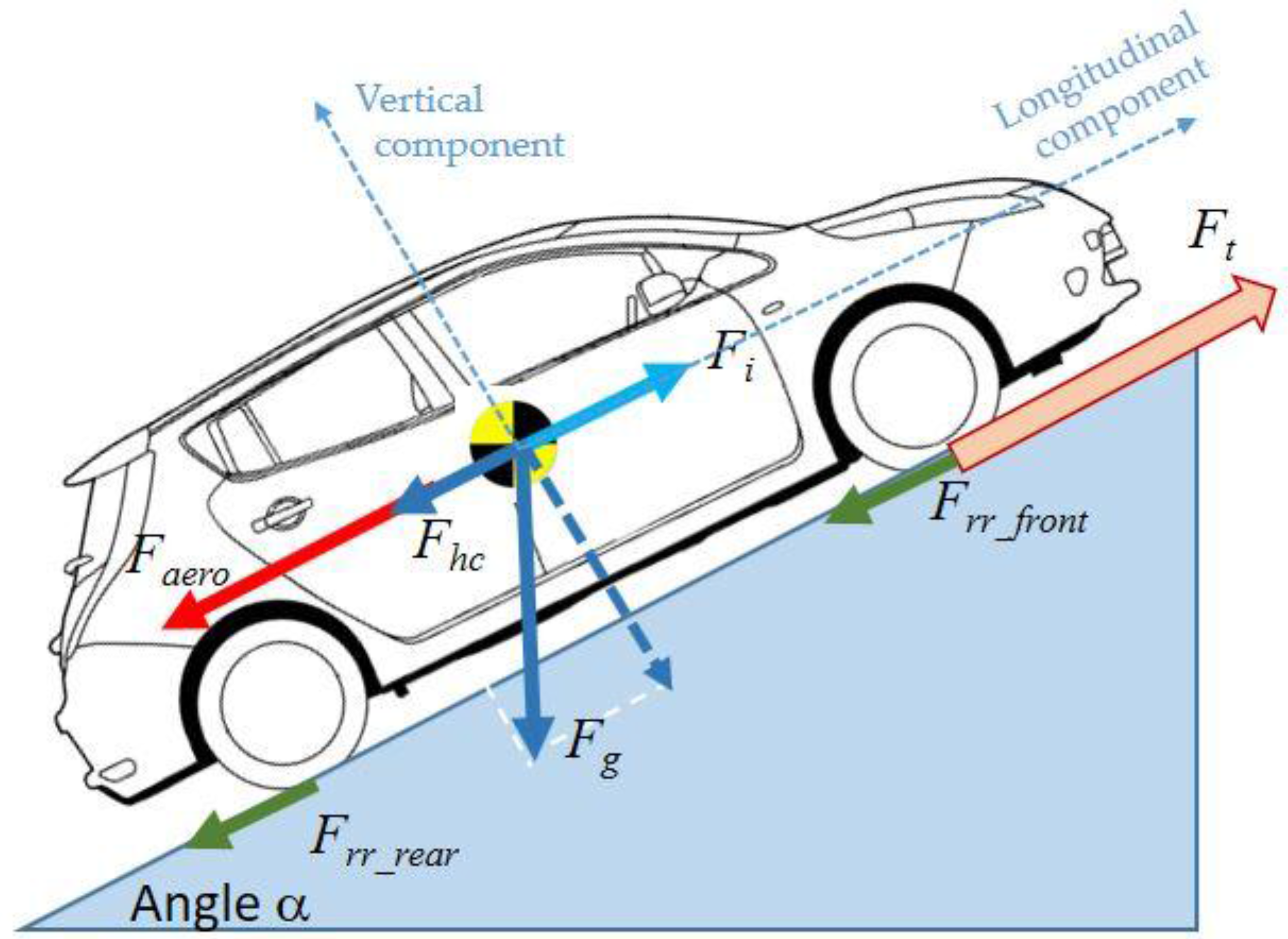
2. Electric Vehicle Consumption Model

This section describes the modeling of the electric vehicle (EV) developed to estimate its energy consumption. The model is based on the direct application of the Newton’s second law for the longitudinal dynamics of the vehicle, as it is shown in Figure 2.

According to the principle of force balance presented in Equation (1), the traction force, F_t, generated by the electric motor, must overcome the sum of all resistive forces acting on the vehicle: the rolling resistance force of the wheels, F_rr; the hill climbing force, F_hc (which is the component of the vehicle weight, F_g, that acts along the slope); the aerodynamic drag, F_aero and the inertial force, F_i:

$$F_t=F_i+F_{\mathrm{hc}}+F_{\mathrm{rr}}+F_{\mathrm{aero}}$$

(1)

The aerodynamic drag is given by Equation (2):

$$F_{\mathrm{aero}}=\mathrm{sign}\left(v+v_{\mathrm{wind}}\right)\frac{1}{2}\rho {AC}_d{(v+v_{\mathrm{wind}})}^2$$

(2)

where A is the front area of the vehicle (in m²), C_d is the aerodynamic drag coefficient, ρ is the air density of dry air (in kg/m³) and v and v_wind are the velocity of the vehicle and the headwind speed respectively [20]. In this work, it is assumed that wind speed is negligible compared to the vehicle’s speed, therefore, v_wind = 0 as it was also proposed in other previous works [21,22,23,24,25].

The rolling resistance forces are acting in all tires, as it is shown on the left side of Figure 2. The resultant rolling resistance force, F_rr = F_{rr_front} + F_{rr_rear}, is given in Equation (3):

$$F_{\mathrm{rr}}=\mathrm{sign}\left(v\right)\left(M_{\mathrm{car}}+M_p\right)g\cos \left(\alpha \right)c_{\mathrm{rr}}$$

(3)

where c_rr defined the tire rolling resistance coefficient, M_car is the mass of the vehicle, M_p is the mass of the people in the vehicle (driver plus passengers), g is the gravity acceleration (9.81 m/s²) and α is the angle of the driving surface (in rad). The rolling resistance coefficient depends on the tire pressure, the road surface type, the road conditions, the vehicle tire type and the linear velocity. In this work, this coefficient is approximated by Equation (4) according to [24]:

$$c_{\mathrm{rr}}=0.01\left(1+\frac{v}{100}\right)$$

(4)

Equation (5) defines the hill climbing force which represents the force required to drive the vehicle up the slope:

$$F_{\mathrm{hc}}=\left(M_{\mathrm{car}}+M_p\right)g\sin \left(\alpha \right)$$

(5)

Finally, Equation (6) represents the inertial force of the vehicle, representing the force required to accelerate the vehicle, where a is its linear acceleration. An additional correction factor, C_i0, must be included in this equation to consider the force needed to provide angular acceleration to the rotating parts. In this work, this value is 0.05 as it is suggested in other similar references [18,19,20]:

$$F_i=C_{i0}\left(M_{\mathrm{car}}+M_p\right)a$$

(6)

The mechanical tractive power at the wheels, P_t, required to drive the vehicle at speed v is given by Equation (7):

$$P_t=F_{t}v$$

(7)

The output power of the battery is computed as:

$$P_{\mathrm{bat}}=\frac{P_t}{{\eta }_{\mathrm{gear}}·{\eta }_{\mathrm{motor}}}+P_{\mathrm{aux}}$$

(8)

where P_aux represents the variable auxiliary loads (heating, air conditioning, radio, lights, etc.), η_gear is the driveline efficiency and η_motor is the electric controller-motor efficiency [18,19,27].

This output power of the battery is evaluated at each time step. During normal forward driving (traction mode), P_t > 0 and P_bat > 0 during a time interval ∆t and the energy (defined by P_bat·∆t) is extracted from the battery, flowing to the wheels.

During the breaking process, EVs recover a significant fraction of the breaking energy, recharging the battery. The input power injected in the battery, P_bat < 0, during this period will depend on the regenerative braking factor, k, as follows:

$$P_{\mathrm{bat}}=k{\eta }_{\mathrm{gear}}·{\eta }_{\mathrm{motor}}{P}_t+P_{\mathrm{aux}}$$

(9)

Note that, in this braking mode, P_t < 0 and:

$$\left|k{\eta }_{\mathrm{gear}}·{\eta }_{\mathrm{motor}}{P}_t\right|>\left|P_{\mathrm{aux}}\right|\to P_{\mathrm{bat}}<0$$

(10)

The regeneration factor, k, which determines the percentage of the total braking power which can be practically recovered is speed-dependent function as it is shown in the following equation [22,24]:

$$k=\{\begin{array}{cc}0.5·v& v<5\mathrm{m}/\mathrm{s}\\ 0.5+0.015\left(v-5\right)& v\ge 5\mathrm{m}/\mathrm{s}\end{array}$$

(11)

The total energy demand of a trip can by computed by:

$$E_{\mathrm{trip}}=\frac{1}{{\eta }_{\mathrm{bat}}}{\int }_{t_0}^{t_{\mathrm{end}}}{P}_{\mathrm{bat}}·\mathrm{dt}$$

(12)

where η_bat is the battery efficiency and t₀–t_end are the initial and final times of the trip. In this work, the input data for the model are vehicle trajectories (second-by-second vehicle speed and position that were recorded by the GPS receiver installed in the smartphone), therefore Equation (12) is discretized as follows:

$$E_{\mathrm{trip}}=\frac{1}{{\eta }_{\mathrm{bat}}}{\displaystyle \sum }_{k=1}^N{P}_{\mathrm{bat}}\left[k\right]·\Delta t$$

(13)

where ∆t is the time span between two consecutive position samples and N is the number of recorded position samples.

The model under study is a Nissan Leaf (2016 version). This vehicle is powered by an 80 kW synchronous motor with a nominal 30 kWh lithium ion battery pack. The values of the main parameters of this model are summarized in

Table 1. Vehicle characteristics.

Description	Symbol	Value
Cross sectional area (m2)	A	2.3316
Curb weight (kg)	Mcar	1521
Driver and passengers’ weight (kg)	Mp	160 (1 driv. + 1 pass.)–230 (1 drv. + 2 pass.)
Nominal battery capacity (kWh)	Cnom	30
Driveline efficiency (%)	ηgear	0.95
Controller and motor efficiency (%)	ηmotor	0.98
Battery efficiency (%)	ηvat	0.98
Auxiliary power load (kW)	Paux	0.2

.

Model Extension to Include Significant Driving Events

In order to derive a more accurate consumption model, small variations in the previous longitudinal dynamics model (defined by Equations (1)–(13)) are proposed. Two available inertial sensors in the smartphones are used in this work: accelerometers and gyroscopes. The first type of sensor measures linear acceleration of movements along the x, y and z axes (including gravity), while the gyroscope measures the rotational velocity (the rate of rotation) around the x, y and z axes.

The linear acceleration is directly used in the longitudinal dynamics model through Equation (6), but the information provided by the gyroscopes is not directly included in the previous model. This information is critical to evaluate different driving behaviors and it will have a direct influence in the energy demanded by the EV. For that reason, in this work the modification of Equations (4) and (6) to include this effect is proposed.

When the vehicle is subjected to abrupt turns, the friction between the tire and the road increases, therefore, it is proposed to modify the weight of the rolling resistance coefficient defined in Equation (4), weighting it by the energy content included in the rotation signal, named E[event] and a constant coefficient K₁ which it is calibrated using Least Squares Method (LSM). The more energetic the turn is, the more friction will occur, increasing the losses:

$$c_{\mathrm{rr}\_\mathrm{mod}}=\left[0.01\left(1+\frac{v}{100}\right)\right]K_{1}E\left[\mathrm{event}\right]$$

(14)

Similarly, when making abrupt movements with the vehicle, the effective moment of inertia of the vehicle will change, increasing the effort to be rotated and increasing the inertial force. This effect will be included by the modification of the additional correction factor, C_i0 in Equation (6), weighting it by the energy content of the rotational signal and a constant coefficient K₂:

$$C_i=K_2{C}_{i0}E\left[\mathrm{event}\right]$$

(15)

3. Data Acquisition, Detection, Classification and Validation

3.1. Data Acquisition and Preprocessing

This method relies on inertial sensors signals, such as accelerometer signals or gyroscope signals. These sensors are obtained from a smartphone, which can be placed anywhere inside the vehicle and may change its position during the recordings with no impact on the accuracy of the results as it will be explained later.

As the hardware for each device is different, we will follow the recommendations given in [15] in order to sample inertial signals at 5 Hz. The devices installed in smartphones are very heterogeneous, therefore, signals could have empty samples. To overcome this limitation, signals are linearly interpolated. These signals are low-passed filtered by using a third order Butterworth filter, in order to erase spurious samples or high-frequency samples not related to driving maneuvers. In this filtering, accelerometer signals are filtered using a cutoff frequency of 1 Hz, whereas gyroscope signals are filtered using a cutoff frequency of 0.25 Hz since with gyroscopes we are less interested in fast variations.

Accelerometer data is affected by Earth’s gravity force. This effect is estimated and removed from the signals, as explained in [15], by applying a decomposition of the 3-dimensional signal into a vertical projection, where the effect of the gravity is estimated, and another projection onto the horizontal plane, where signals must be affected only by driving events. These two projections are presented in Figure 3 for a given segment. In the upper plot, the vertical projection is shown, where the signal represents the vertical force as, for instance, the gravity force. It is remarkable that the signal has an offset at 9.8 m/s² because gravity force is constant, variations around this offset represent the incidence of other vertical forces (potholes, bumps, etc.). In the bottom plot, the horizontal plane projection is represented, where all forces related to driving events are present. On this horizontal plane projection there in no offset because no constant force affects the device measurement.

3.2. Events Detection

As smartphone devices are not in a fixed position, manipulations of the devices are possible. These manipulations could mask the signals referring to simple driving events. In order to clean these from the signal, manipulations are detected when the gyroscope signal is too strong to be a driving maneuver. These uncontrolled movements are removed from the signal and, then, the system is recalibrated since the position of the device has changed, and the projections depicted in previous section are obtained again.

For gyroscopes, once the manipulation events have been removed, and after verifying that there are no stationary signals affecting them, the sum of the filtered energy is obtained as representative of driving behavior.

Once the signal is clean, it is assumable that all high energy events are related to driving events so a threshold over the driving noise level, being this noise level the signal when the car is moving straight without accelerating nor braking, is set up. The calculation of noise threshold has been made by means of the median. This threshold is selected in both horizontal plane projections of accelerometers and total energy of gyroscopes, as explained in [15]. Once the horizontal plane projection signal of accelerometer or the total energy of gyroscopes exceed the threshold, an event has been detected.

3.3. Events Classification

To categorize the driving style, we discover the existence of maneuvers, then we establish what kind of maneuvers are performed and, finally, if these maneuvers are abrupt or not. Every event detected is classified according four main categories: left turns, right turns, accelerations and braking; although the types of maneuvers could be divided into more subcategories.

Other classification techniques could be used, but neural networks have proved to be one of the most useful tools to classify activities with sensors. One of the important decisions for the training of the network is to decide which input signals are to be used, selecting those ones coming from the smartphone sensors, with the exception of GPS signal because it could increase considerably the battery consumption of the device. To translate one driving event into one of the four maneuvers mentioned above, we decided to simplify the model and use only six input signals; the components [X, Y, Z] of the accelerometers and the components [X, Y, Z] of the gyroscope.

In Figure 4 an example of a driving maneuver is presented. The upper plot depicts the accelerometer signals and the lower plot the gyroscope signals. The Z axis on accelerometer signals represents the vertical component, besides integrating the offset from the gravity force. The X and Y axes define the horizontal plane, thus variations of the signal on this place imply that there is a driving event to be taken into account. The lower plot shows a variation on the Z axis of the gyroscope, meaning that the car is turning around the vertical axis: a turn event is taking place.

First of all, we will begin with a database of signals previously labeled as left and right turns, accelerations and braking. This database will be used as training input for a neural network of some dense layers, with a fully connected layer and a softmax regression layer to the output to return probabilities of the four previously mentioned categories.

For the training of the network, as “ground truth”, we use data from a set of car trips with additional information from an OBD device installed in the car. This tool accurately recreates a vehicle trip and analyzes user’s driving incidents measuring precisely accelerations to notify of drivers’ harsh braking, acceleration and turn events. With this event information coming from the OBD, we have been able to correctly classify and synchronize the maneuvers detected by means of the analysis of signals from the smartphone, determining events of different length and type, according to the aforementioned categories.

Between the different neural network options, we have decided to use a recurrent neural network (RNN), in particular a Long-Short Time Memory (LSTM). These types of networks are appropriate for time series modeling as is the case of accelerometer signals.

One of the main differences between a LSTM networks and a standard RNN, is that the nodes of the LSTM networks are memory cells. The memory cells have self-recurrent connections and three control gates: input gate (to write), output gate (to read) and forget gate (to reset). These gates are the ones that will allow updating cell states in each step of time, storing possible temporal relationships along time.

Therefore, detected maneuvers, from the analysis of smartphone sensor data (see example Figure 5), will be introduced into the LSTM network as inputs in raw data, without any type of preprocessing. In every time step t, a new input will be received to the network, a_t, and the memory will be updated, s_t. Each input, a_t, will be captured at the same time instant, t, along six channels, three coming from the accelerometers and three from the gyroscope. The memory will be updated through the cell state, by aggregating the old memory (forget gate) and the new memory (input gate): i.e., the forget gate will control what information will be kept (remembered) and what information will be skipped (forgotten), whereas the input gate will control what information of the input signal (in this time t) will be added. Finally, the output gate will decide what information will pass to the next time step (t + 1). In summary, in each time t, an output of the network will be provided, calculated upon the current input and previously processed information.

We have chosen an LSTM network of two stacked layers, with the output sequence of one layer forming the input sequence for the next. Each LSTM layer has 64 neurons. When a large amount of data is available, the results can be greatly improved when the number of stacked layers is increased. However, this significantly increases the number of parameters and consequently the memory and processing capacity required. Therefore, although we have performed the processing on a computer equipped with a Nvidia Tesla K80 graphic card (instead of the smartphone), for practical reasons the layers have been limited to two and the neurons by layer to 64, offering good results with reasonable resource requirements. At the output of the recurrent network, there will be a fully connected feed forward-layer to classify the input maneuvers into our four classes (left turns, right turns, accelerations and braking) and a softmax layer, providing the probability in each time instant. To build the neural network we have used the open source software library TensorFlow^TM with Python.

To validate the results, cross-validation tests have been performed to ensure that the results are independent of the partition between training and testing. In particular, a k-fold cross-validation was performed, with a k = 3. Data in each iteration are divided into three subsets, using each subset as testing and others as training successively; and the final error will be the average of the errors obtained. The number of drivers, routes and maneuvers used for such training is shown below (

Table 2. Training database.

Description	Value
Drivers	68
Routes	22,194
Total maneuvers	16,029
Total left turn maneuvers	4649
Total right turn maneuvers	4907
Total braking maneuvers	3498
Total acceleration maneuvers	2975

).

With a total of 68 different drivers and an average of 326 routes by driver, we have considered that it is a heterogeneous database for the tests. The final model uses an Adam optimizer for minimizing the cross-entropy loss function, backpropagating the gradients from the softmax layer through to the input layers. Finally, the validation accuracy has been around 79%.

Therefore, the raw signals coming from the sensors of mobile device will be captured, by means of the process of detection of events suggested in the previous section we will capture events susceptible of being turns (left or right) or accelerations or braking, being braking an acceleration event but with an opposite sign. With the trained database we will evaluate what kind a maneuver is. However, not all maneuvers are equally useful when mapping them in the model of energy consumption. Therefore, we are going to focus on the abruptness of the events without making any difference between left and right turns, and between accelerating or braking events. To categorize the maneuvers according to their abruptness a value of abruptness is given obtained from the maximum of accelerometer energy inside the event.

3.4. Events Validation

In order to adjust the proposed mathematical model, several trips during 3 weeks where recorded using a 2016 Nissan Leaf. In Figure 6 it is shown the installation of a Bluetooth On-Board Diagnosis II (OBDII) scanner which was plugged into the Leaf’s OBD port to register several pieces of information available from the CAR-CAN bus. A special software named LeafSpy Pro was used to analyze the data read from the vehicle and store it in a .CSV file. The main registered variables were the following:

• “Date/Time”
• “Latitude and Longitude” in the following format: dd mm.yyyy
• “Elv” Elevation in meters.
• “Speed” in the km/h.
• “Gids”, which indicates the energy in the Nissan Leaf battery (current capacity = 80 Wh.Gids)
• “SoC” State of Charge (SoC) of the Traction Battery.
• AHr” Capacity of the Traction Battery.
• “Pack Volts” Traction Battery voltage
• “Pack Amps” Traction Battery amperage, which is positive when the current is extracted from battery (during driving), or negative when Regen or charging.
• “Odo (km)” Odometer reading in kilometers.
• “SOH” The State of Health of the Battery in percent.
• “epoch time”, where one sample represents the time in seconds from 1 January 1970.
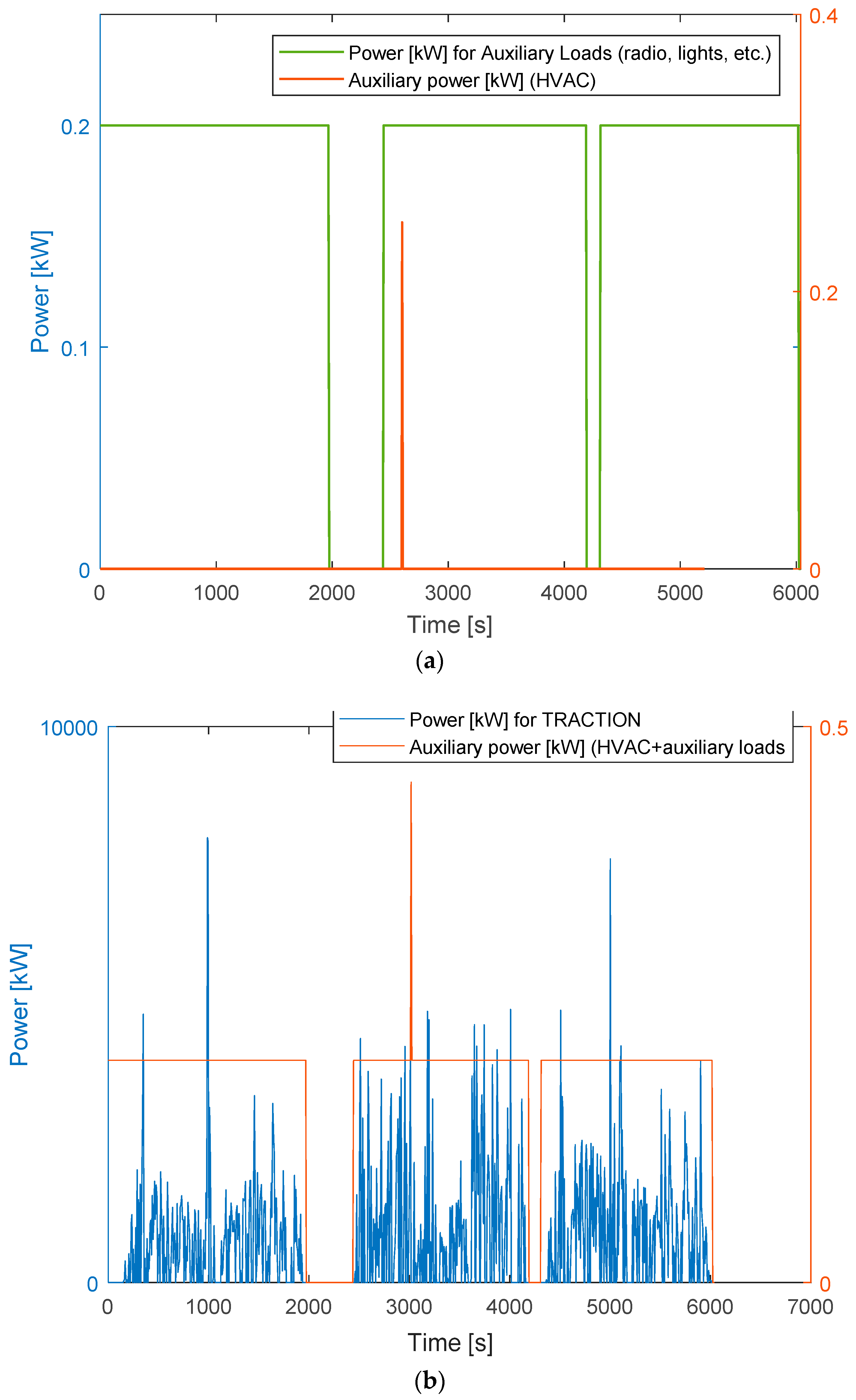
• “Motor Pwr (100 w)” Drive motor power.
• “Aux Pwr (100 w)” Power used by the auxiliary equipment (Lights, Radio, Navigation system, rear defroster…).
• ”A/C Pwr (250 w)” Power used by the Air Conditioning System power.
• “Gear” “7” Gear position (0 = not read yet; 1 = Park; 2 = Reverse; 3 = Neutral; 4 = Drive; 7 = B/Eco)

4. Results

The main results of this work are included in this section. Initially, a model validation based on one specific driving cycles: the EPA Urban Dynamometer Driving Schedule (UDDS) is presented.

Then, all registered trips were classified using a k-means scheme, splitting them in three different categories representing: (1) smooth driving, (2) aggressive driving and (3) mild driving styles. The consumption results of three representative trips (one for each cluster) are also shown (selected as the closest trip to the cluster centroid).

4.1. Initial Model Validation

According to the official data [28], the nominal range of this vehicle is up to 107 miles (172.2 km) under the 2017 LA4 driving cycle. The estimated range by the proposed model under the same driving cycle is 170 km. The driving profile of the first two cycles and the initial evolution of the State of Charge (SoC) are presented in Figure 7.

4.2. Real Trip Validation

To validate the results with real conditions, we performed a total of 50 trips, and classified them using a simple clustering scheme (k-means clustering) which can lead to three different categories: smooth driving, including a reduced number of events (cluster 1); aggressive driving including a high number of events (cluster 2); and mild driving, including an average number of events (cluster 3).

All trips were done using the same driving setup in the car to avoid driving biases. These trips were made on the same circuit of 24 km (mix of city and roadways), varying the conditions of the vehicle (increasing the weight) and the driving style.

After the clustering, we selected representative candidates of the clusters by selecting the ones with closest distance to the centroid cluster, and comparing the model with real results. Then, we selected three different representative trips of the clusters. These three trips were made consecutively, on the same 24 km circuit, varying the conditions of the vehicle (increasing the weight) and the driving style.

In order to evaluate only the influence of the driving behavior on the proposed model, the total consumption and the consumption of all auxiliary loads have been recorded. Then the power used to propel the vehicle has been obtained (subtracting the consumption of all auxiliary loads to the total consumption).

Figure 8a shows the total auxiliary loads during these three consecutive trips. This consumption has two different components, the first one is due to the conventional auxiliary loads (navigation systems, radio, etc.) and it remained almost constant at around 0.2 kW. The second component is due to the HVAC System. This system was disconnected during the experiment at it is observed in the figure, but the air conditioning was suddenly connected/disconnected during the second trip to register this event, which is observed as a 0.25 kW peak at 3018 s.

Figure 8b shows the traction power and the total auxiliary loads. It is observed that the traction power is variable depending on the driving conditions.

Figure 9 presents the different events detected by the app. Blue stems represents acceleration/braking events, orange-brown stems indicate turn events (to the left or to the right) and finally, green stairs shows the stop periods. All stems signals are weighted by their total energy, therefore, the longer the stem, the greater the contained energy and the higher their abruptness.

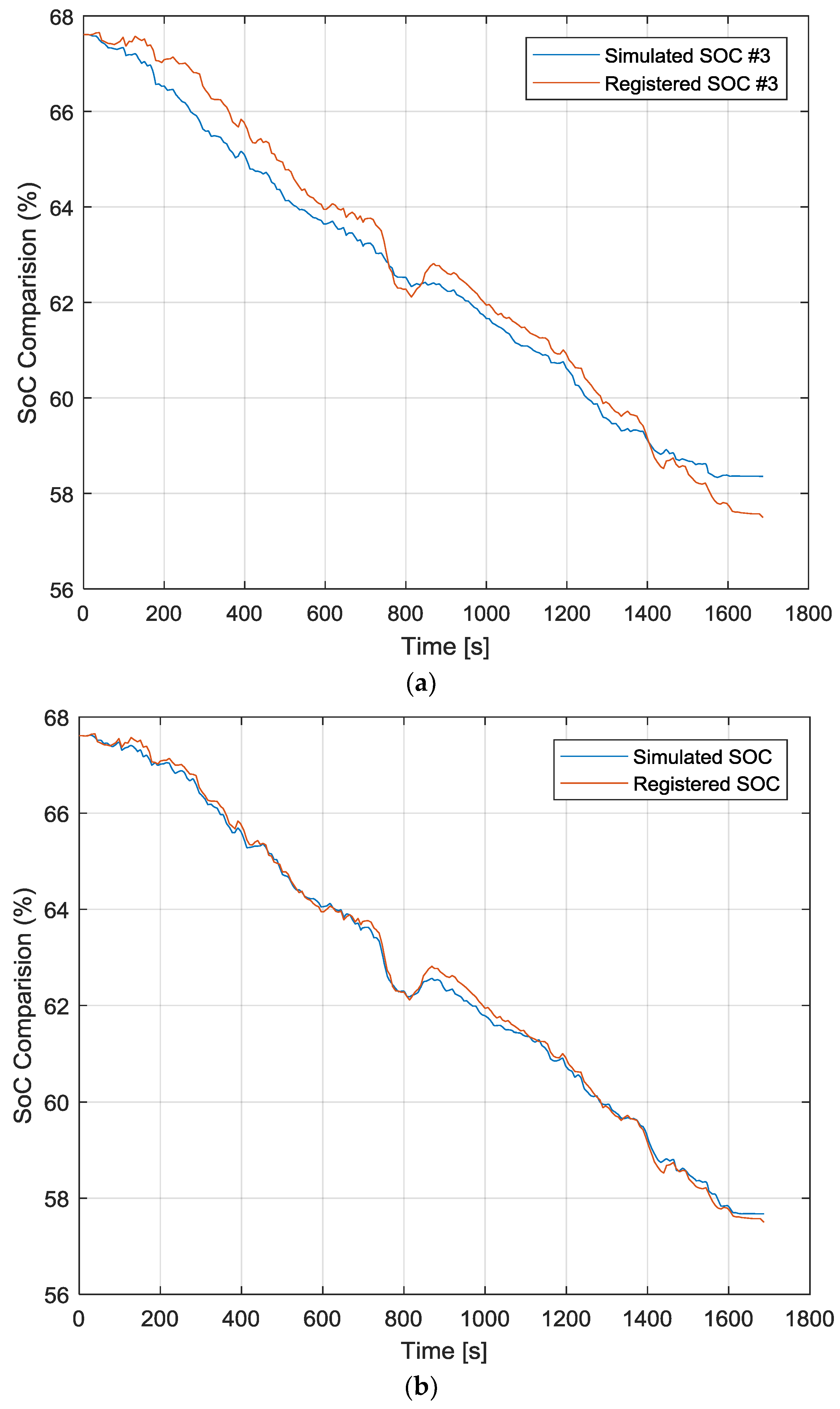
4.2.1. Cluster 1 (Smooth Ride) Representative Trip

This initial trip was performed with a driver and a single passenger (M_p = 160 kg). Figure 10 shows the detected events (Figure 10a) and the speed and elevation profile (Figure 10b) for this first trip.

The results are presented in Figure 11, where the elevation profile is considered in both simulations. Figure 11a presents the result of the first simulation scenario, where the driving events were not initially considered in the model. It is observed that the energy consumed by the simulation model is 2.497 kWh while the real energy consumption registered was 2.5575 kWh. The average consumption simulated was 102.9539 Wh/km, while the average consumption registered was 105.4008 Wh/km. The mean square error was 0.4182.

Figure 11b presents the result of the simulation considers both driving events (acceleration and turning events). It is observed that the energy consumed by the simulation model is 2.588 kWh while the real energy consumption registered was 2.5575 kWh. The average consumption simulated was 106.6572 Wh/km, while the average consumption registered was 105.4008 Wh/km. The mean square error was 0.191.

4.2.2. Cluster 2 (Aggressive Driving) Representative Trip

This trip included an additional passenger (incrementing the total weight of the car compared to the former trip, M_p = 230 kg). Figure 12 shows the detected events (Figure 12a) and the speed and elevation profile (Figure 12b) for this second trip).

The results are presented in Figure 13, where again, the elevation profile has been considered in both simulations. Figure 13a presents the results of the first simulation scenario, which does not include the driving events, and it is observed that the energy consumed by the simulation model is 3.0054 kWh while the real energy consumption registered was 3.565 kWh. The average consumption simulated was 123.389 Wh/km, while the average consumption registered was 146.3635 Wh/km. The mean square error was 0.44229.

Figure 13b shown the response of the proposed consumption model during the second simulation scenario (including all detected driving events, shown in Figure 12a). It is observed that the energy consumed by the simulation model is 3.391 kWh while the real energy consumption registered was 3.565 kWh. The average consumption simulated was 139.22 Wh/km, while the average consumption registered was 146.3635 Wh/km. The mean square error was 0.4422.

4.2.3. Cluster 3 (Mild Driving) Representative Trip

The initial condition of this trip is equal to the previous one, with the same number of passengers (one driver and two passengers, M_p = 230 kg). Figure 14 shows the detected events (Figure 14a) and the speed and elevation profile (Figure 14b) for this third trip).

The final results are presented in Figure 15, where both simulation scenarios include the elevation profile. In Figure 15a the driving events have not been considered, while in Figure 15b all driving events for the third trip are included in the model. It is observed, in the first scenario (without driving events), the energy consumed by the simulation model is 2.7758 kWh while the real energy consumption registered was 3.1775 kWh. The average consumption simulated was 113.0258 Wh/km, while the average consumption registered was 129.3805 Wh/km. The mean square error was 0.4731.

During the second scenario (considering all driving events shown in Figure 14a), the energy consumed by the simulation model is 2.9812 kWh while the real energy consumption registered was 3.1775 kWh. The average consumption simulated was 121.3863 Wh/km, while the average consumption registered was 129.3805 Wh/km. The mean square error was 0.12482.

5. Conclusions

Climate change is currently one of the main challenges facing the international community. It is a phenomenon whose environmental, economic and social causes and consequences, intimately linked with the current model of economic development, require new solutions that allow a better management of energy. The progressive introduction of electric vehicles is one of the key factors in the change of the energy model, and accurate information on consumption and use models, is essential to correctly assess its impact. Moreover, the application of Big Data techniques to this field leads to a better comprehension of the context, so the acquisition of the greatest amount of information is a key process and smartphones are a perfect fit for this purpose.

The use of smartphones sensors has resulted in a simple way to obtain info from the vehicle, including abrupt driver behavior events which are useful to improve the consumption model of electrical vehicles, and allow a personalized estimation of range without involving intrusive systems. They allow the solution to be universalized without being linked to specific hardware that represents a barrier to entry.

Thus, an accurate, and efficient energy consumption model has been implemented providing information for real-time eco-driving systems that can enhance the energy efficiency of EVs. The proposed model can be easily integrated into richer modeling frameworks including different levels of transport electrification and traffic simulation.

With the presented application and the training of the neural networks with more than 22,000 trips it was demonstrated that it is possible to classify abrupt events into left-right turn events, acceleration events and braking events. A value of abruptness can be also assigned to each event, which is useful for such personalized energy consumption models. In any case, it opens the field for future research regarding the impact of these kind of events and driving behaviors on the traffic flow. Concerning the validation with the real consumption, representative trips were chosen to be simulated by the proposed model.

The results show that including the driving behavior in this model can improve the accuracy by up to 50%. Three different scenarios were simulated, corresponding to three driving behaviors. In the first scenario (smooth ride), the total error between the simulated consumption and the real registered was reduced from 2.36% (if the abrupt events were not considered) to 1% (if the events were considered). In the second scenario (aggressive ride), the total error was reduced from 15.7% to 4.8%. Finally, in the last scenario (mild ride), the total error was reduced from 12.6% to 6.17%. The accuracy of the model is reduced when the driving style become more aggressive. Even in this more aggressive condition, the simulation that includes the events modeling provides a better response than the model that does not include such events.

References

1. International Energy Agency. Global EV Outlook: Understanding the Electric Vehicle Landscape to 2020; International Energy Agency: Paris, France, 2013. [Google Scholar]
2. International Energy Agency. Global EV Outlook 2017; International Energy Agency: Paris, France, 2017; Available online: https://www.iea.org/publications/freepublications/publication/GlobalEVOutlook2017.pdf (accessed on 8 February 2018).
3. Drivesapp. Available online: www.driviesapp.com (accessed on 8 February 2018).
4. Plötz, T.; Hammerla, N.Y.; Olivier, P. Feature learning for activity recognition in ubiquitous computing. In Proceedings of the IJCAI, International Joint Conference on Artificial Intelligence, Barcelona, Spain, 16–22 July 2011; Volume 22, pp. 1729–1734. [Google Scholar]
5. Yao, S.; Hu, S.; Zhao, Y.; Zhang, A.; Abdelzaher, T. Deepsense: A unified deep learning framework for time-series mobile sensing data processing. In Proceedings of the 26th International Conference on World Wide Web, Perth, Australia, 3–7 April 2017; International World Wide Web Conferences Steering Committee: Geneva, Switzerland, 2017; pp. 351–360. [Google Scholar]
6. Giannotti, F.; Nanni, M.; Pedreschi, D.; Pinelli, F.; Renso, C.; Rinzivillo, S.; Trasarti, R. Unveiling the complexity of human mobility by querying and mining massive trajectory data. VLDB J. Int. J. Very Large Data Bases 2011, 20, 695–719. [Google Scholar] [CrossRef]
7. Wahlström, J.; Skog, I.; Händel, P. Driving Behavior Analysis for Smartphone-based Insurance Telematics. In Proceedings of the 2nd Workshop on Physical Analytics, Florence, Italy, 22 May 2015; ACM: New York, NY, USA, 2015; pp. 19–24. [Google Scholar]
8. Phan, T. Intelligent Energy-Efficient Triggering of Geolocation Fix Acquisitions Based on Transitions between Activity Recognition States. In Mobile Computing, Applications and Services; Springer International Publishing: Basel, Switzerland, 2013; pp. 104–121. [Google Scholar]
9. Oshin, T.O.; Poslad, A.; Ma, A. A method to evaluate the energy-efficiency of wide-area location determination techniques used by smartphones. In Proceedings of the IEEE 15th International Conference on Computational Science and Engineering, Nicosia, Cyprus, 5–7 December 2012; pp. 326–333. [Google Scholar]
10. Dunlap, S. Persistent Location Tracking on Mobile Devices and Location Profiling. Patent US 20130085861 A1, 4 April 2013. [Google Scholar]
11. Basir, O.A.; Jamali, S.H.; Miners, W.B.; Toonstra, J. Method of Correcting the Orientation of a Freely Installed Accelerometer in a Vehicle. Patent US 20130081442 A1, 4 April 2013. [Google Scholar]
12. Van Ly, M.; Martin, S.; Trivedi, M.M. Driver Classification and Driving Style Recognition using Inertial Sensors. In Proceedings of the IEEE Intelligent Vehicles Symposium (IV), Gold Coast, Australia, 23–26 June 2013. [Google Scholar]
13. Johnson, D.A.; Trivedi, M.M. Driving Style Recognition Using a Smartphone as a Sensor Platform. In Proceedings of the 14th International IEEE Conference on Intelligent Transportation Systems (ITSC), Washington, DC, USA, 5–7 October 2011; pp. 1609–1615. [Google Scholar]
14. Fazeen, M.; Gozick, B.; Dantu, R.; Bhukhiya, M.; González, M.C. Safe Driving Using Mobile Phones. IEEE Trans. Intell. Transp. Syst. 2012, 13, 1462–1468. [Google Scholar] [CrossRef]
15. Pozo, R.F.; Gomez, L.A.H.; Meco, D.L.; Vercher, J.B.; Muñoz, V.M.G. Method for Detecting Driving Events of a Vehicle Based on a Smartphone. Patent US 20160016590 A1, 21 January 2016. [Google Scholar]
16. Alvarez, A.D.; Garcia, F.S.; Naranjo, J.E.; Anaya, J.J.; Jimenez, F. Modeling the driving behavior of electric vehicles using smartphones and neural networks. IEEE Intell. Transp. Syst. Mag. 2014, 6, 44–53. [Google Scholar] [CrossRef]
17. Meseguer, J.E.; Toh, C.K.; Calafate, C.T.; Cano, J.C.; Manzoni, P. Driving styles: A mobile platform for driving styles and fuel consumption characterization. J. Commun. Netw. 2017, 19, 162–168. [Google Scholar] [CrossRef]
18. Larminie, J.; Lowry, J. Electric Vehicle Technology Explained, 2nd ed.; John Wiley & Sons: Chichester, UK, 2012; ISBN 978-1-119-94273-3. [Google Scholar]
19. Ehsani, M.; Gao, Y.; Gay, S.E.; Emadi, A. Modern Electric, Hybrid Electric, and Fuel Cell Vehicles: Fundamentals, Theory, and Design, 2nd ed.; CRC Press LLC: Boca Raton, FL, USA, 2016. [Google Scholar]
20. Schaltz, E. Electric Vehicles—Modelling and Simulations. In Electric Vehicles-Modelling and Simulations; Soylu, S., Ed.; InTech: London, UK, 2011; p. 487. ISBN 978-953-307-477-1. [Google Scholar] [CrossRef]
21. Asamer, J.; Graser, A.; Heilmann, B.; Ruthmair, M. Sensitivity analysis for energy demand estimation of electric vehicles. Transp. Res. Part D Transp. Environ. 2016, 46, 182–199. [Google Scholar] [CrossRef]
22. Genikomsakis, K.N.; Mitrentsis, G. A computationally efficient simulation model for estimating energy consumption of electric vehicles in the context of route planning applications. Transp. Res. Part D Transp. Environ. 2017, 50, 98–118. [Google Scholar] [CrossRef]
23. NREL (National Renewable Energy Laboratory). FASTSim: Future Automotive Systems Technology Simulator. 2014. Available online: https://www.nrel.gov/transportation/fastsim.html (accessed on 8 February 2018).
24. Fiori, C.; Ahn, K.; Rakha, H.A. Power-based electric vehicle energy consumption model: Model development and validation. Appl. Energy 2016, 168, 257–268. [Google Scholar] [CrossRef]
25. Alves, J.; Baptista, P.C.; Gonçalves, G.A.; Duarte, G.O. Indirect methodologies to estimate energy use in vehicles: Application to battery electric vehicles. Energy Convers. Manag. 2016, 124, 116–129. [Google Scholar] [CrossRef]
26. Zhang, R.; Yao, E. Electric vehicles’ energy consumption estimation with real driving condition data. Transp. Res. Part D Transp. Environ. 2015, 41, 177–187. [Google Scholar] [CrossRef]
27. Lee, C.-H.; Wu, C.-H. A Novel Big Data Modeling Method for Improving Driving Range Estimation of EVs. IEEE Access 2015, 3, 1980–1993. [Google Scholar] [CrossRef]
28. Available online: https://www.nissanusa.com/electric-cars/leaf/versions-specs/ (accessed on 8 February 2018).
Figure 1. Drivies app.
Energies 11 00412 g001
Figure 2. Free body diagram of the different longitudinal forces acting on the vehicle.
Energies 11 00412 g002
Figure 3. Decomposition of 3-dimensional accelerometer signal: (a) vertical projection. (b) horizontal projection.
Energies 11 00412 g003
Figure 4. (a) Example of a turn maneuver in a real driving detention. (b) Top plot represents signals from accelerometer sensor. (c) Bottom plot represents signals from gyroscope sensor.
Energies 11 00412 g004
Figure 5. Smartphone sensor signals will be input of a neural network with a fully connected layer and a softmax layer like outputs to provide probabilities associated to each maneuver.
Energies 11 00412 g005
Figure 6. (a) 2016 Nissan Leaf. (b) Location of the OBD port (c) Installation of the Bluetooth OBDII scanner (d) Smartphone location inside the vehicle during the trips.
Energies 11 00412 g006
Figure 7. EPA LA4 driving cycle consumption estimation.
Energies 11 00412 g007
Figure 8. (a) Total auxiliary loads (b) Traction power and Auxiliary power (in [kW]) for the three consecutive trips.
Energies 11 00412 g008
Figure 9. (a) Detected events of the three representative trips. (b) Zoom over an area with events.
Energies 11 00412 g009
Figure 10. (a) Detected events during Trip #1 (b) Speed and elevation profiles during Trip #1.
Energies 11 00412 g010
Figure 11. Trip #1 (a) Driving events, shown in Figure 9, are not considered in this simulation (b) Driving events are considered.
Energies 11 00412 g011
Figure 12. (a) Detected events during Trip #2 (b) Speed and elevation profiles during Trip #2.
Energies 11 00412 g012
Figure 13. Trip #2 (a) Driving events, shown in Figure 11, are not considered in this simulation (b) Driving events are considered.
Energies 11 00412 g013
Figure 14. (a) Detected events during Trip #3 (b) Speed and elevation profiles during Trip #3.
Energies 11 00412 g014
Figure 15. Trip #3 (a) Driving events, shown in Figure 13, are not considered in this scenario (b) Driving events are considered in this scenario.
Energies 11 00412 g015