Aircraft Noise Assessment—From Single Components to Large Scenarios
by
 , , and
Jan Delfs
1, 
Lothar Bertsch
1,
Christoph Zellmann
2,
Lennart Rossian
1,
Ehsan Kian Far
3,
Tobias Ring
3 and
Sabine C. Langer
3,* 1
DLR, Institute of Aerodynamics and Flow Technology, 38108 Braunschweig, Germany
2
Laboratory for Acoustics/Noise Control, Empa - Swiss Federal Laboratories for Material Science and Technology, 8600 Dübendorf, Switzerland
3
TU Braunschweig, Institute for Engineering Design, 38106 Braunschweig, Germany
*
Author to whom correspondence should be addressed.
Energies 2018, 11(2), 429; https://doi.org/10.3390/en11020429
Submission received: 14 December 2017
/
Revised: 30 January 2018
/
Accepted: 30 January 2018
/
Published: 13 February 2018
(This article belongs to the Special Issue Towards a Transformation to Sustainable Aviation Systems)
Abstract
:The strategic European paper “Flightpath 2050” claims dramatic reductions of noise for aviation transport scenarios in 2050: “...The perceived noise emission of flying aircraft is reduced by 65%. These are relative to the capabilities of typical new aircraft in 2000...”. There is a consensus among experts that these far reaching objectives cannot be accomplished by application of noise reduction technologies at the level of aircraft components only. Comparably drastic claims simultaneously expressed in Flightpath 2050 for carbon dioxide and NOX reduction underline the need for step changes in aircraft technologies and aircraft configurations. New aircraft concepts with entirely different propulsion concepts will emerge, including unconventional power supplies from renewable energy sources, ranging from electric over hybrid to synthetic fuels. Given this foreseen revolution in aircraft technology the question arises, how the noise impact of these new aircraft may be assessed. Within the present contribution, a multi-level, multi-fidelity approach is proposed which enables aircraft noise assessment. It is composed by coupling noise prediction methods at three different levels of detail. On the first level, high fidelity methods for predicting the aeroacoustic behavior of aircraft components (and installations) are required since in the early stages of the development of innovative noise reduction technology test data is not available. The results are transferred to the second level, where radiation patterns of entire conventional and future aircraft concepts are assembled and noise emissions for single aircraft are computed. In the third level, large scale scenarios with many aircraft are considered to accurately predict the noise exposure for receivers on the ground. It is shown that reasonable predictions of the ground noise exposure level may be obtained. Furthermore, even though simplifications and omissions are introduced, it is shown that the method is capable of transferring all relevant physical aspects through the levels.
1. Introduction
Global mobility is greatly supported by transport aircraft and their capability of long range operation and high traveling speeds. Nevertheless, the acceptance for airborne transport is strongly affected by the noise exposure of the residents, especially in the surrounding of the airport [1,2,3]. This is accounted for by “Flightpath 2050”, a report of the European Commission providing a roadmap and goals for future civil aircraft development. In this context, one major aim of “Flightpath 2050” is the reduction of the perceived noise by 65% for flying aircraft [4]. Hence, it is necessary to assess the noise emission of new aircraft designs in combination with effective low noise technologies from the viewpoint of the receiver, i.e., a resident in the vicinity of an airport. Within this contribution, a multi-level, multi-fidelty approach is presented that aims to assess aircraft designs on the basis of noise exposure levels on the ground and thereby favors a perception-focused approach rather than a technologically driven one. With this method available, two main goals become achievable: Firstly, new aircraft may be designed and optimized regarding not only their direct noise emission but also in view of their contribution to the overall ground noise exposure levels. Secondly, new aircraft and airport operation procedures may be designed and optimized in order to cope with concurring goals, such as economic and ecologic efficiency. Furthermore, the multi-level, multi-fidelity approach can be extended to incorporate other sound sources, e.g., road and rail noise.
An appropriate aircraft noise assessment requires precise data on several levels, as it should account for the sources directly at the aircraft itself (level one) as well as flight paths (level two) and operation procedures (level three) [5]. This knowledge can be gathered for existing aircraft, but is hardly available during the design phase. Furthermore, aircraft design, operation procedures and other aspects might influence each other, as new aircraft designs might require new operation procedures or flight paths [6,7].
On the first level, the sound emission from aircraft components is computed based on flow computations around these components using computational fluid dynamics (CFD) methods [8]. Typically, the results serve as input to codes which compute the aeroacoustics using computational aeroacoustic (CAA) methods [9]. This procedure leads to high levels of prediction accuracy, but is restricted to small computation domains in comparison to a complete aircraft or even large scale scenarios with many aircraft on different flight paths. The next level is of greater scale but otherwise less detailed and aims for the prediction of the sound exposure on the ground for single aircraft. For this purpose, the sound emission of the dominant sound sources at the aircraft is being superimposed in order to form an overall aircraft radiation pattern. As the aircraft exhibits different flight configurations during a complete take-off-cruise-landing cycle, the radiation pattern is computed for all relevant configurations. On the last and coarsest level, radiation patterns are propagated to the ground for distinct flight paths and thus form a long-term noise footprint describing an entire scenario. Finally, noise footprints of such scenarios with many aircraft and other traffic types are superimposed in order to predict the overall noise exposure of residents on large time scales, for example a year of operation.
Within this contribution, a multi-level, multi-fidelity approach is presented that inherently couples domain-specific numerical tools of all three aforementioned levels of detail and thereby composes a chain, which enables the prediction of noise exposure on the ground due to present and future aircraft including sound propagation from the source to the receiver. With this method available, new low noise aircraft design technologies become assessable at the receiver location using perception-focused quantities. This possibility provides a great benefit for aircraft design regarding the goals of “Flightpath 2050”. The objective of this contribution is to demonstrate this seamless prediction/assessment concept on the application of some noise reduction technology vs. a low noise aircraft configuration.
On the first level, this chain is composed of the CFD code TAU, developed at DLR (DLR—German Aerospace Center (Deutsches Zentrum für Luft- und Raumfahrt)), and CAA code PIANO (Perturbation Investigation of Aerodynamic NOise), developed at DLR, for computing the noise emission on component level. The tool PANAM (Parametric Aircraft Noise Analysis Module), developed at DLR, computes the noise emission of entire aircraft for different flight configurations in level two. In level three, the aircraft noise simulation tool sonAIR, developed at Empa, is used to perform the calculation of sound propagation as well as to superimpose the noise of many single aircraft in entire scenarios. This chain as well as the coarsening of the modeling through the different levels is depicted in Figure 1. The tools are described in more detail in Section 2.
The following working hypotheses form the basis for the proposed procedure and shall be verified using preliminary numerical studies:
- Existing tools for noise prediction of different levels of complexity (i.e., component level, single aircraft level, system scenario level) can be coupled in order to aim for a resource efficient description of the noise exposure on the ground due to aircraft traffic.
- The coupling of the different levels forms an integral description of the entire problem that preserves the relevant physical relations even though the model is coarsened considerably from component to scenario noise assessment.
- The direct connection of the single models on each level enables the correlation of changes in the aircraft design and noise exposure levels on the ground. This gives the opportunity to assess and optimize aircraft design with a perception-focused approach, as required for Flightpath 2050.
Noise exposure prediction due to aircraft noise usually works on the second or third level of the proposed procedure with, depending on the tool to be used, information from previous levels typically insufficiently incorporated in subsequent levels. Therefore, the presented work aims on coupling all levels from aircraft design to noise exposure prediction. In total, an automated assessment of low-noise technology over all three levels is achieved. As each of these levels incorporates different orders of detail and very different methods, the first hypothesis to be verified is concerned with the possibility of coupling these levels in order to form a description of the entire problem that can be evaluated efficiently.
The second hypothesis relates to the problem of information loss. The aim of predicting noise exposure on the ground requires an adequate setup of the whole model. The presented method provides a model that is made up of different levels of complexity that are being coupled. Thereby, information is propagated through the levels of the entire model. As the levels are being coarsened from each level to the subsequent ones, information is lost or omitted. This information loss will result in erroneous results. Thus, the second hypothesis claims that the information transferred through the levels is sufficient in order to generate reasonable results that account for the main effects properly.
Changes in aircraft design which alter the aircraft noise emission result in measurable effects for the ground noise level. Therefore, hypothesis number three assumes that these effects can be computed using the proposed method of coupling different prediction tools with different levels of detail.
2. Prediction Concept—Approach and Methods
In the following section a detailed description of the different tools that are being used for the multi-level tool chain depicted in Figure 1 is given. Thus, in Section 2.1 the CFD and CAA methods of level one are described that enable the noise emission computation on component level. The results of dominant noise sources are used in level two in order to assemble the overall source noise radiation patterns of entire aircraft as described in Section 2.2. Within the third level, as described in Section 2.3, these patterns are used to predict noise footprints for single operating aircraft. Finally, these footprints are superimposed for large scale scenarios and noise exposure levels on the ground for distinct receiver locations are computed.
2.1. Noise Assessment of an Aircraft Component (Level 1)
Noise assessment of aircraft components can be accomplished using numerical and experimental investigations. Typically, for new technologies no measured aeroacoustic data is available on aircraft components. Furthermore, the effort to set up e.g., comprehensive aeroacoustic wind tunnel tests usually is very high, slow and costly. Semi-empirical source models, as used for system noise prediction tools (e.g., PANAM tool, used in level two, see Section 2.2), are typically based on some theoretical concept and a calibration with measured data. For the lack of such data and in view of a seamless numerical assessment of new technologies, it is mandatory to provide the relevant aeroacoustic database for a technology on the basis of efficient, high fidelity CAA simulations.
For the work presented, a CAA concept is pursued, which is non-empiric because it does not assume any preset geometry or component, thus general enough on the one hand and very efficient due to modeling on the other hand, to provide fast enough response times. This concept is hybrid in the sense that initially a RANS (Reynolds-averaged Navier-Stokes) flow field simulation is done with DLR’s CFD Code TAU [10]. The second step consists of two parts, (a) the stochastic unsteady 3D modeling of the turbulence by DLR’s stochastic turbulence generator fRPM (fast Random Particle Mesh Method) [11,12] and (b) the actual CAA computation of the (acoustic) perturbation field about the given RANS flow field by means of DLR’s CAA code PIANO [13], see Figure 2.
The approach requires an appropriate modeling of the unsteadiness of turbulence, which means that it has to cover those features of the turbulence which are relevant for the sound generation, see [14,15]. The respective turbulence representation is realized with the stochastic turbulence generator “fRPM” which takes the flow field and one point turbulence statistics from a pre-cursor RANS mean flow simulation as an input. The convection characteristics are met correctly, while the given distribution of the turbulence kinetic energy k, and a local correlation length is satisfied. A typical computational setup is shown in Figure 3. Turbulence is only realized in the relevant source domain (called “fRPM source patch”, see [14,15]) as shown in Figure 3a. A snapshot of the resulting sound pressure field is plotted in Figure 3b for illustration. The source region is discretized by a Cartesian mesh with an appropriate resolution of to resolve the turbulent structures which determine the number of mesh points, typically ranging around numbers of for 2D simulations. As discussed in [14,15], the dynamic of the synthesized turbulence is represented by an ensemble of particles, moving along in the (given) mean flow provided by the RANS CFD solution. The number of particles required to represent the turbulent eddies typically is slightly larger than the number of mesh points in 2D. The mesh for the acoustic propagation (solution of the APE—“Acoustic Perturbation Equations”, ref [16]) is set to resolve acoustic wavelengths of the desired maximum frequencies with 7 points per wavelength.
Although the turbulence is stochastically realized in 3D, for 2D geometries like a slat the CAA computations may be carried out in a wing section in 2D since spanwise velocity fluctuations do not contribute to the generation of slat noise. This approach enables very fast computation and thus short turn around times (a few hours on a work station) to determine spectral differences of systematically varied slat configurations. In general one may state that this approach is valid for any flow whose time average can be described appropriately based on the RANS flow model.
2.1.1. Level 1 Interface to Level 2 (Full Aircraft Prediction)
The predicted sound pressure spectra of design variants are related to the spectrum of the respective (standard) reference aircraft component. The resulting spectral difference is transferred to the level two prediction. This “delta” information is used to accordingly modify the level two prediction model of that component as a function of observer orientation and flight condition, implemented as a look-up table. In case that a low noise technology affects the aerodynamics of the aircraft, respective corrections are to be extracted from the level one simulations and transferred to level two as well.
2.1.2. Validity of Level 1 Prediction for Slat Noise Reduction Technology
The above mentioned component noise prediction concept is demonstrated on the example of the noise generated at the leading edge of a transport aircraft’s wing in high lift configuration, i.e., when the leading edge slats and the trailing edge flaps are deployed for landing. During this phase of flight, the high lift system of a modern, say Airbus A320 type, transport aircraft is a very important source of community noise. In fact, together with the deployed landing gear, the slat can dominate the aircraft overall noise at the certification location “approach”. This is particularly true for aircraft equipped with high bypass ratio turbofan engines (e.g., A320 NEO).
Slat noise is a very difficult problem to simulate numerically, since its origin is the presence of turbulence in the strongly accelerated flow through the slot between slat and main element. Low noise targeted design modifications are practically impossible to carry out with scale resolving approaches such as “Large Eddy Simulation” (LES) since the number of required simulations would lead to unrealistic computation times.
In the following, the validity of the CAA approach described in Section 2.1 for slat noise is demonstrated by comparison to acoustic data, measured in DLR’s Acoustic Wind tunnel Braunschweig (AWB), see Figure 4. In Figure 5, the results of a systematic slat gap and overlap variation (definitions see Figure 4b) are shown. The low noise slat setting was found by simulation of a large set of gap and overlap positions. The reference and the variant exhibiting least noise were implemented into DLR’s research high lift airfoil model F16 with a chord length of and a span of in AWB (see Figure 4). The prediction of the one-third octave band spectra corresponds well with the measured result and the difference in spectra between reference and the low noise setting are predicted very accurately. Only in the very low frequency domain the results differ due to parasitic noise originating from the wind tunnel background noise. The data shows that the computation concept for slat noise is valid and may be used for different slat designs. In Section 3.1.1 this method will be used to predict the noise reduction achieved by re-designing the slat to a so called “very long chord slat” (VLCS) [17].
A second noise reduction technology for high lift noise, which will be implemented in the overall assessment is the concept of a so called “slat cove liner”, described in more detail in Section 3.1.2. In this case the noise reduction is not accomplished by manipulating the local flow and therefore the sound generation. Instead, present slat sound is absorbed by a liner, placed in the nearfield of the slat source, namely in the cove area. For this reason, this technology will be further referred to as “slat cove liner”.
Although this noise reduction technology was found experimentally on the F16 slat, its application to different high lift leading edge devices is of high interest. In other words, not only the source noise reduction by the shaping of the slat is to be covered by the numerical prediction approach, but simultaneously the effect of a cove liner. A respective prediction capability was developed within the German Corporate Research Center CRC880, funded by the German research council DFG. For this purpose, the equations solved within the prediction chain shown in Figure 2, are extended by extra terms which model the presence of porous volumes. DLR’s RANS solver TAU [18] and perturbation solver PIANO [19,20,21] were re-formulated in volume-averaged form to describe the presence of porous material in a homogenized way. This results in the occurrence of extra modeling terms in the momentum equations, so called Darcy and Forchheimer terms, involving the permeability (inverse flow resistance) and porosity (volume fraction of air of connected pores) of the material. For a validation of the approach to be used in Section 3.1.2, see [21].
2.2. Noise Assessment of a Single Aircraft (Level 2)
In the context of the evaluation of acoustic properties of novel aircraft technology, the term aircraft system noise is used. According to Burley [22] aircraft system noise is defined as the “source noise emitted by an aircraft in flight, propagated through the atmosphere, and received by observers or sensors on the ground”. Consequently, the aircraft noise emission has to be simulated in a first step. As the noise emission of separated sources is covered by the numerical investigations in level one as described in Section 2.1, level two provides the overall noise radiation patterns of single aircraft for every necessary flight configuration by combining the single sources of level one. Within this contribution, this is done using the DLR-tool PANAM [23].
When simulating the noise emission, it is assumed that the overall aircraft noise emission can adequately be approximated as the sum of the most relevant individual noise sources/components on-board, thus a component approach is pursued. Thereby, individual relevant noise sources are modeled separately and certain interaction effects are accounted for to finally assemble the overall aircraft noise emission.
The selected noise source models are parametric with respect to the aircraft/engine design parameters and the aircraft operation. This is a prerequisite if different vehicle concepts along various flight procedures are to be investigated. The quantity and complexity of the required input data is still manageable and available in the early conceptual design phase.
The overall aircraft noise is separated into airframe and engine noise contribution. Selected airframe noise source models have been developed by DLR as described in previous literature [24,25]. These DLR in-house models describe the major noise sources and some dominating interaction effects. Explicit models for the simulation of major turbofan engine noise sources are available from literature. PANAM predicts turbofan engine noise as a combination of the two dominating noise sources jet and fan, respectively. Stone’s model [26] is employed for the jet noise originating from the core and bypass jet. For the fan noise simulation the Heidmann model [27] is applied. The empirical database of the original Heidmann model has been modified in order to reflect more recent developments in the field of engine fan design. Possible shielding effects of the engine fan noise are considered using the DLR ray-tracing tool SHADOW [28]. The application of SHADOW allows to study promising low noise aircraft concepts with significantly reduced fan noise contribution.
PANAM usually is applied to perform the aircraft system noise prediction for all selected aircraft design concepts along their individual flight trajectories (an example can be seen in Figure 6a). Within the presented simulation process, PANAM is applied to predict emission levels of single aircraft as input for level three. Furthermore, the ground noise predictions of PANAM are used to optimize the flight trajectory of each aircraft which is also a required input to level three. Furthermore, PANAM can be included as a module within the PrADO (Preliminary Aircraft Design and Optimisation Program) [29] simulation process so that all the required input data for a noise prediction can be generated as described by Bertsch [23]. At this point, the process can readily be applied towards medium-range, conventional transport aircraft with turbofan or propeller engines.
2.3. Noise Assessment of System Scenarios (Level 3)
In this step, the authors study the effect of new technologies within entire airport scenarios with the scope to minimize the noise distribution on ground. For this purpose, the aircraft noise simulation tool sonAIR [31] is applied. The tool comprises of a sound source database and a sound propagation model, which are formulated for one-third octave bands within a frequency range of 25 Hz to 5 kHz.
The sound source database was developed for fast calculations using the sound emission model described in [32], which predicts the sound emission of turbofan powered aircraft as a function of the flight configuration (power setting, Mach number and aeroplane configuration, i.e., flaps, slats and landing gear). The database consists of two look-up tables for airframe and engine noise sources, where the sound emission levels are stored as a function of frequency, directivity and flight parameters. This interface is used to implement PANAM outputs from the second level to sonAIR. Thus, the description of the sound source is still very detailed and the loss of information is small.
For the calculation of the sound propagation, a hybrid modeling approach is implemented in sonAIR. In case of simple situations, where direct sound is dominant, only geometric divergence and atmospheric absorption and a mean ground effect are accounted for. In other cases, where the sound incidence angles are low, the sound propagation model sonX can be applied to account for effects as shielding (due to e.g., buildings, topography), ground reflections or foliage attenuation. However, for the proof of concept in this paper, the sound propagation is simplified to direct sound as the topography is simplified, too.
For the task of noise mapping, calculations are performed for a receiver grid with a constant height above the ground. In aircraft noise simulations, typically numerous single flights are processed together resulting in a footprint, i.e., the sound exposure averaged over a bundle of flights, on all receiver points arranged in a grid. In Figure 6b an example of a noise footprint during take-off is given, indicated by the . However, the quantity to be considered within this contribution is the , meaning the A-weighted exposure level. As a last step, these footprints are weighted with the number of movements per aircraft and route and the contributions from all aircraft and route combinations are energetically summed up.
The sonAIR-software is embedded into a geographic information system (Esri ArcGIS), in which the input data as well as the results are stored and visualized. Such environment also facilitates comparisons of noise contours or statistics on the number of affected people (e.g., high annoyance, sleep disturbance).
3. Application
In the following section, an overview of the application of the proposed coupling concept for aircraft noise assessment is given. First, the low noise airframe technologies, “VLCS” and “slat cove liner”, as investigated in level one are presented. In the following, three aircraft concepts and their corresponding flight paths are being described. The aircraft concepts cover the state of the art as well as a specifically designed low noise concept. Furthermore, the investigated scenario, which is a derivative of the standardized SANC-TE scenario, is discussed.
3.1. Low Noise Airframe Technologies
In this section two airframe noise reduction technologies on slat noise (very long chord slat and slat cove liner) will be predicted by means of the computation chain presented in Section 2.1. In order to be manageable, only difference spectra between the reference (standard) high lift system and the two new technologies are provided to level two as described in Section 2.1.1. In this way, the level two prediction (PANAM) may still use its standard (semi-empirical) prediction models for the various aircraft components and only applies level differences. In this case the DLR slat noise model available for standard slats will be modified. When studying the source noise reduction potentials of modifications to a high lift system component it is important to consider the effects on the aerodynamic performance simultaneously. For instance, the slat position variation (see validation Section 2.1.2) usually reduces the maximum achievable lift coefficient with the section lift force, the freestream air density, the freestream flow speed, and c the airfoil chord. Although primarily represents an aerodynamic performance indicator, the noise source is affected indirectly as well. The maximum lift coefficient determines the stall speed of the aircraft and due to regulations the actual minimum allowable landing speed is a set proportional to this stall speed . Therefore, any reduction in the performance of the high lift system leads to the necessity that the aircraft flies faster upon approach. Taking into account that the slat sound intensity scales with shows that the aerodynamic high lift performance indeed affects the sound actually radiated from the high lift system. This example shows that the aerodynamic characteristics of any considered low noise modification of a high lift system additionally influences the overall noise characteristics of the aircraft. Consequently, not only the acoustic data, but aerodynamic data determined in the level one analysis as well need to be transferred to the level two computations in order to enable a correct overall noise prediction and a fair comparison among variants.
While in future applications, the method for overall noise prediction as proposed in this work will deal with entirely unknown, new technologies, here two technologies are applied, which are known to reduce source noise. Respective source noise reductions have been measured in acoustic wind tunnel tests. The point here is to show that an entirely predictive computation chain has been successfully established, that is capable of assessing aircraft component technologies down to the noise environment at the airport. The low noise technologies considered within this contribution were chosen deliberately in order to avoid negative effects regarding the aerodynamic performance of the high lift system.
3.1.1. Very Long Chord Slat (VLCS)
By elongating the slat chord considerably, the overlap of the slat trailing edge and the main wing front part is increased. This has two potentially positive consequences on the noise radiation. Assuming most sound to originate from the slat trailing edge, the positioning of this edge over the main airfoil will provoke acoustic shielding, so that less sound is radiated towards the ground. This is mostly an acoustic installation effect. Since slat sound is not only generated by eddies passing by the slat trailing edge, but to a considerable part by the acceleration of turbulent eddies in the mean flow as fluid gets pushed through the slat slot (see [33]), the VLCS reduces this acceleration. One reason is, that the acceleration from stagnation to maximum speed takes place over a longer path compared to the standard slat. As mentioned, one important feature of the VLCS is, that it features about the same aero-performance as the reference F16 airfoil. Figure 7 shows the noise reduction result of using this VLCS, as measured on an aircraft half model in the NWB acoustic wind tunnel of DNW (Deutsch-Niederländische Windkanäle) at DLR in Braunschweig, Germany. It should be noted that the noise reduction is on the order of 5–7 dB in a broadband sense. This already indicates that in this case it is reasonable to apply a constant modification of the standard slat noise model spectra used in the level two prediction code PANAM (see Section 3.2).
The CAA simulation of the reference F16 and the VLCS airfoils is based on the CAA Code PIANO involving the turbulence generator fRPM as described in Section 2.1. In this particular case, the source region (“source patch”) is discretized by a Cartesian mesh with a resolution of (with c the chord length of the airfoil with retracted leading and trailing edge devices). In order to represent the relevant turbulent structures, 90,000 mesh points were used along with a total of 100,000 single particles that represent the turbulent eddies convecting inside of the source patch. The CAA mesh for the acoustic propagation is set to resolve frequencies up to with 7 points per wavelength, resulting in approximately 720,000 points. The resolutions are very similar for the reference airfoil F16 and the one with the VLCS.
The results obtained from the computation chain support the experimental findings. Figure 8a illustrates the overall noise reduction obtained by the VLCS configuration when compared to the F16 reference airfoil. A substantial decrease in the sound pressure level can be observed for the entire computational domain. The directivity of the radiated sound is only slightly changed due to a different slat angle and angle of attack ( for F16 and for VLCS) as may be observed in Figure 8b. Therefore one may assume that the noise reduction is practically omnidirectional. Figure 9 shows the spectral noise reduction evaluated below the airfoil. It shows, that a significant reduction of around 8 dB is achieved on average mainly on low to mid frequencies. Deviations to the experimental reduction result shown in Figure 7 are attributed to the fact that measurement results were determined from microphone array based source localization data integrated over a section of a 3D tapered aircraft wing, while the simulations represent a 2D ideal situation. Nevertheless, the assumption of a broadband noise reduction of for the level two predictions appears reasonable.
3.1.2. Slat Cove Liner
The slat cove liner concept has been developed within a research activity called “Move-On”, funded by the German Ministry of Economics (BMWI) within the national German research programme “Lufo”. According to various material combinations, an open foam type insert into the slat cove structural volume was found to give best results. This material was covered with a so called “duo-layer mesh”, which is a fine woven metal mesh of the producer “Spoerl” [35]. The cove side of the slat of the F16 high lift airfoil of DLR was equipped with this foam insert and the duo-layer mesh face sheet and tested in the AWB and later on validated for a large 4:1 scale model in DNW’s Large scale Low speed Facility LLF. The configuration used for the computational approach is sketched in Figure 10.
Figure 11 shows the result of the noise reduction obtained in the experiments. Here, a broadband noise reduction of about 3 dB is observed. In comparison, Figure 9 illustrates the noise reduction predicted by the computational approach. Therewith, an almost constant reduction of about 2 dB is found. This deviation from the experimental results can be related to differences in the geometry on the one hand and uncertainties of the flow resistance through the actual liner on the other. It is particularly interesting to note that the noise reduction by the slat cove liner may be expected to act in addition to any noise reduction obtained on the source by re-designing the shape or setting of the slat. The reason is, that the reduction principle is just to absorb the sound of the slat, no matter whether or not it originates from a high or a low noise slat design.
3.2. Aircraft Concepts
Specific existing aircraft concepts have been selected for an initial application of the simulation process. The vehicles under consideration are based on previous research findings toward low noise aircraft. These vehicle concepts are (1) a reference aircraft similar to a conventional A319 aircraft, in the following referred to as “V-R” and (2) a low-noise design. The two aircraft configurations are depicted in Figure 12a,b, respectively. As it can be seen, both configurations mainly differ in the assembling topology of the wings and engines. Both vehicles have been subject to a dedicated noise assessment in previous research activities, for example in [23]. For the V-R, fan noise has been identified as the dominating noise source along departure and as a relevant source along most of the approach. Based on this outcome, the low noise design has been specifically designed to shield the fan noise and thereby enable a significant noise reduction along both departure and approach [23].
Yet, significant reduction of the fan noise leaves a prominent role for the airframe noise contribution, especially along the approach flight path. Consequently, the basic versions have been further modified in order to reduce the increasing importance of airframe noise contribution by adding low noise airframe technology as described in Section 3.1.1 and Section 3.1.2 and furthermore with modifications to the landing gear [36]. Thus, three aircraft types, the reference aircraft V-R, the modified reference aircraft, in the following referred to as "retrofit" and the modified low noise configuration, in the following referred to as "gamechanger" are to be investigated within this study. The following technologies have been applied to the modified configurations:
- Landing gear mesh fairing.
- Porous flap side edge.
- Low noise slat technologies.
For this preliminary study it is assumed, that these technologies do not influence take-off weight or induce aerodynamic penalties. The predicted emission spectra for landing gear, flap, and slat noise have then been modified according to previous findings or the high-fidelity computational results from Section 3.1. The predicted one-third octave emission spectra for each noise source, i.e., landing gear, flap and slat have been reduced by constant delta levels. The predicted landing gear noise is reduced by , the flap noise emission spectra is reduced by . Based on high-fidelity computations, the VLCS (see Section 3.1.1) technology is accounted for by a conservative level reduction of compared to the reference design.
Using these assumptions the noise emission spectra can be predicted for various operating conditions for a predefined reference distance. The emission data contain one-third octave spectra for discrete emission angles all around the aircraft. Exemplary emission plots are depicted for the reference aircraft (V-R) and the “gamechanger” under identical operating conditions. For an approach configuration see Figure 13a and for a departure configuration see Figure 13b. The corresponding operation parameters are provided in the figure. In the diagrams, the sound pressure level depending on the different angles and on an enveloping surface is shown, where the flight direction is denoted by and the direction of the wings is denoted by , respectively (see Figure 14). Moving source effects, e.g., the convective amplification, are included in the emission data. The departure case clearly demonstrates the effect of fan noise shielding for the “gamechanger”. Significant noise level reductions can be achieved in forward direction due to the selected engine installation. By the approach emission data the effect of the low-noise airframe technology is demonstrated. Obviously, airframe noise is dominating the overall aircraft noise for the selected approach condition.
Specific interfaces allow the translation of this emission data into the input format of sonAIR, which is comprised of a separate description of airframe and engine noise emission spectra for each operating condition and emission angle. Multiple PANAM runs are then executed in order to fill up the defined emission database as required by sonAIR to describe each aircraft in a simulation run. The sonAIR input data are comprised of PANAM emission results for 7 different flight altitudes, 5 flight Mach numbers, 6 high-lift configurations and 7 engine settings.
3.3. Trajectories
Finally, all three aircraft, i.e., V-R, “retrofit” and “gamechanger”, are simulated along tailored flight paths accounting for their individual flight performance [11]. Figure A1 and Figure A2 in the Appendix A show the simulated flight trajectories. It can be seen that all vehicles are forced to fly on nearly identical altitude profiles. Since no aerodynamic or weight penalties are accounted for, the V-R and “retrofit” yield identical flight trajectories. The “gamechanger” results in a slightly different flight path regarding thrust setting and airspeed due to different aerodynamics and weights compared to the reference vehicle. These approach and departure flight paths are then again translated into a corresponding sonAIR input format in order to enable the flight simulation. Finally, each vehicle can now directly be modelled in sonAIR according to its individual emission database and along its individual flight procedure. The three vehicles along their defined approach and departure flights can now be integrated into a larger airport scenario as simulated with sonAIR. Thus, the gap between level two and level three is closed. The scenario used within this work is described in the following section.
3.4. Scenario
The considered airport scenario for a first application example is adopted from the Swiss Aircraft Noise Calculation Test Environment (SANC-TE) [37]. The test environment allows comparing different aircraft noise prediction software on a standardized basis in Switzerland. For this reason, it provides input data such as idealized flight trajectories including dispersion tracks, the number of movements and sound emission data for a given set of aircraft types. All aircraft that are accounted for in the SANC-TE scenario are given in Table 1. It also contains the considered movements along the flight routes for departure (TD00-TD05) and approach (TA01, TA02) for all aircraft in the scenario (see Figure 15b). The calculated scenario corresponds to the airport scenario AP001S01, which is adequate to integrate the three aircraft concepts of the previous section.
An overview of the given airport scenario including runway, flight paths and topography is shown in Figure 15a. The input data including the flight path names (see Table 1) used in this work are shown in Figure 15b. The runway is defined by SANC-TE with a length of and the sound exposure is calculated on an area of across with a receiver mesh size of . Each of the six departure and two approach flight paths is divided into one backbone track and six sub-tracks. The spacing of the subtracks and the percentage of movements are based on a normal distribution function following Doc. 29 [38]. The topography includes an artificial hill in the south and a mountain ridge in the north. The sound propagation is based on a homogeneous atmosphere (ambient temperature , atmospheric pressure , relative humidity = 70%) and simplified to geometric divergence and atmospheric absorption. This simplification is applied to demonstrate the proof of concept. With sonX, effects as shielding (i.e., from buildings, topography) and ground effect can be considered in the future, but on the costs of larger calculation times.
Based on the SANC-TE scenario AP001S01, three variants are taken into account. As the reference case, the sound emission model of the A320 is replaced by the V-R vehicle, which represents the current technology level in use. Consequently, in a second variant the A320 is substituted by the “retrofit” and a third variant uses the “gamechanger”. The number of movements (i.e., the number of flights) is identical for all variants. It should be noted that while the A320 is replaced by the investigated low noise aircraft, all other aircraft that are given in Table 1 remain non-modified in the scenario.
The contingent of each aircraft type of the SANC-TE scenario in Table 1 shows, that the A320 (which is substituted e.g., by the V-R) and MD81 are with 53% the most prevalent aircraft types (92208 out of 175198 movements). Both aircraft exhibit the same number of movements, but the A320 only departs straight or turns to the north whereas the MD81 departs straight or turns to the south. While the sound exposure of V-R and MD81 is similar for approach, the MD81 shows about higher sound exposure levels () below the flight track.
As the new aircraft designs exhibit different flight performances, their individual flight paths differ among each other as well as compared to the flight path of the A320 as discussed before. This results in systematic deviations in the sound exposure levels due to different distances between source and receiver position. Hence, these differences between the various aircraft could not be attributed to the aircraft design itself. In order to work around this issue, for the presented study the predefined flight trajectories of the A320 are used. This modification especially becomes important for the approaches, as the height profiles show large differences, because the simplified SANC-TE flight tracks are not similar to the simulated and physical flight tracks. Thus, identical height profiles are used for all aircraft in order to enable a fair and appropriate comparison of all aircraft designs in this scenario. However, the aircraft airspeed, rotational speed of the low pressure compressor (N1), and the aeroplane configuration are adopted from Section 3.2 and convoluted with the flight trajectories of the A320. This assumption is supposed to be reasonable as all three vehicles are equipped with an engine similar to the one used by A320. With this procedure, the flight parameters are preserved, as they have significant influence on the sound power level.
4. Results
The results presented are based on the predicted -values for all investigated aircraft types. The is the total sound exposure level based on the yearly movements given in Table 1 and averaged over 16 hours of the day (6 to 22 o’clock). Therefore, this comparison reveals the influence of the modified airframe sources of “retrofit” and “gamechanger” vs. V-R in a yearly scenario. In Figure 16, the of the three variants (i.e., V-R, “retrofit” and “gamechanger” substituting the A320) are shown.
The areas with the highest exposure levels are located in the vicinity of the runway, along the approach lines and along the departure routes. The departure route TD04 shows the largest affected area. This seems reasonable, as this route has the most departures of all considered routes. The main differences between the contours for the three investigated aircraft designs are found along the straight approach and departure routes. East and west of the runway, the isolines for V-R (black) show larger levels with increasing distance to the runway in comparison to both, “retrofit” (yellow) and “gamechanger” (green). Thus, an exposure level reduction is obtained. Along the departure routes, only the “gamechanger” provides a reasonable reduction of the exposure levels. This may be explained by the fact that the “gamechanger” is designed to shield the engine noise, which is dominant during departure. As the “retrofit” design aims only on reducing the airframe noise, benefits can only be expected during approach. For the departure routes to the south, no movements of the investigated aircraft types are considered, consequently, no differences are observed among the three variants.
In the northern and southern vicinity of the runway relatively large sound exposure levels can be found. This unusual effect is due to the lack of lateral attenuation within the simplified sound propagation. In future calculations, the lateral attenuation should be accounted for.
In Figure 17, the difference of the ground noise exposure levels () between the variants of the SANC-TE scenario with “retrofit” vs. V-R are shown. The level differences under the flight tracks in distance to the landing threshold are below (area within the black solid line), which represents the local benefit of the “retrofit” aircraft in this scenario. The maximum value is while the benefit is restricted to a distance of (border of the calculation area). Beyond this distance landing gear, slats and flaps are retracted. Therefore, no noise reduction mechanisms are active anymore in these areas. This plot clearly shows, as stated before, that the benefits of the “retrofit” design are limited to the approach as during this period airframe noise is a relevant source. During departure, where engine noise is the dominant source, the “retrofit” design is not beneficial or at least, no benefit can be computed.
The noise exposure level differences between “gamechanger” and V-R are shown in Figure 18. The maximum reduction is as both, benefits from departures and approach contribute to the noise reduction below the approach tracks (east and west of runway). The departures to the north show the isolated effect of the generally quieter aircraft concept “gamechanger”. The benefits below the flight tracks are always below and in two areas below with a maximum at with some distance to the runway.
5. Discussion
Hypothesis number one (see Section 1) focuses on the possibility of coupling methods on different levels of complexity and order of detail (i.e., aircraft components, noise radiation of single aircraft, scenarios with many aircraft). The results presented in Figure 16 show the beneficial properties of low noise aircraft technologies. The quantity of interest is the total noise exposure level on the ground with a scenario of many aircraft movements averaged over a year of operation. The expectation, that low noise aircraft technologies result in a measurable reduction of the ground noise exposure levels, is confirmed with the results, i.e., hypothesis number one is verified. The tool chain of coupled numerical methods with different levels of complexity works and provides reasonable results.
The coarsening of the level of detail from the aircraft component level to subsequent levels results in an information loss and thus in the negligence of physical aspects of the entire problem. Nonetheless, the results presented seem reasonable. This is furthermore substantiated, as the proposed method still uses a high level of detail. The radiation patterns formed in level two are based on semi-empirical source models and delta level spectra (see Section 2.2). Furthermore, the propagation of the results from level two to level three distinguishes between engine and airframe noise provided in one-third octave bands and accounting for main flight parameters, e.g., engine rotational speed and Mach number (see Section 2.3 and Section 3.2). Hence, still a detailed description of the overall aircraft noise emission is achieved. Thus, hypothesis number two can be verified as well, as this hypothesis states that the most relevant physical relations are preserved by the proposed method.
Hypothesis number three states that changes in the aircraft design can be correlated to the ground noise exposure levels. The noise exposure level differences between the reference V-R and the “retrofit” configuration are shown in Figure 17. Significant noise reductions are present in the direct extension of the runway center line, thus, these reductions can mainly be attributed to the approaches. This can be expected, as the aircraft design modifications of the “retrofit” alter the airframe noise only. During departure, engine noise is the dominating source, thus, airframe noise is a relevant source only during approach. This is clearly substantiated by the results presented in Figure 17.
In Figure 18, the noise exposure level differences between the V-R and the “gamechanger” are shown. Compared to the scenario with the “retrofit” configuration, larger areas with significant noise reduction levels can be seen. This is reasonable as the “gamechanger” is equipped with noise reduction technologies for both, airframe and engine noise. Whereas the noise exposure during approach is dominantly reduced by the airframe noise reductions as discussed before, engine noise is the dominant source during departure. The departure routes of the low noise aircraft lead straight on the center line of the runway and with turns to the north. Thus, noise level reductions can be expected along these routes and are provided by the results as shown in Figure 18.
Both, the results of the “retrofit” as well as the “gamechanger” show that the design’s aims are met. The “retrofit” aims on reducing the airframe noise and thus noise reduction only during approach is expected. This is provided by the results. The same holds for the “gamechanger”. This design aims for reducing both, airframe and engine noise. Accordingly, noise reductions during both, approach and departure are expected and substantiated by the results. Hence, hypothesis three is verified as the aircraft designs correlate with the predicted ground noise exposure levels. Furthermore, the results show that noise reduction levels can be computed for entire scenarios with input data generated on aircraft component level and thus give a further verification of the hypotheses one and two. Given these verifications, the method presented seems appropriate for assessing future aircraft designs with regard to the requirements of “Flightpath 2050”.
6. Conclusions and Outlook
The European vision “Flightpath 2050” provides a roadmap and goals for the future of airborne transport systems. Among others, one of the major objective is the reduction of the aircraft noise impact of 65%. The overall aim is the noise exposure reduction for the residents on the ground rather than the more technologically driven (unconditional) reduction of the noise emission only. In order to reduce ground noise efficiently, aircraft technology, aircraft configuration and aircraft operation have to be taken into account simultaneously. Moreover, unconventional aircraft, designed to make future use of renewable energy resources including alternative propulsion concepts need to be assessed in view of their noise impact long before any piece of hardware is manufactured. Any aircraft noise impact prediction tool therefore has to be general enough to cover the noise characteristics of such aircraft and their non-standard technologies. The presented three level approach, strictly based on numerical simulation was assembled to meet this requirement.
Aircraft noise assessment can be accomplished on different levels of complexity. For the aircraft design, the noise emission of separated components such as flaps, slats, landing gear can be computed using high fidelity CAA (computational aeroacoustics) methods. On the next level, aircraft noise emission for entire aircraft can be predicted by superimposing simplified models for all relevant sources including adaptation due to low noise technology. The coarsest level is the prediction of ground noise for entire scenarios with many aircraft. Currently, these levels work independently as the results of higher order levels (i.e., higher level of detail) are not or insufficiently propagated directly to subsequent levels.
The presented paper deals with the coupling of numerical methods on the aforementioned levels of detail in order to aim for an aircraft noise assessment that uses human-focused quantities as success measures. On level one, CAA computations using the DLR code PIANO are used to predict the noise emission of separate aircraft components. These results are used in level two within the DLR code PANAM to predict the noise emission of entire aircraft to form radiation patterns accounting for all relevant flight parameters, e.g., airspeed, power setting. The commercial tool sonAIR is used on level three to compute the noise exposure levels on the ground for the representative SANC-TE scenario using one reference and two low noise aircraft configurations. The reference configuration is a standard aircraft layout representing the current technology level in use. The first design (called “retrofit”) is identical to the reference, but equipped with low noise measures such as low noise flaps and slats. The second low noise aircraft (called “gamechanger”) furthermore additionally aims for the shielding of engine noise by mounting the engines above the wing.
Results are presented for both, the input data obtained from CAA computations on component level and the overall results of the proposed method, i.e., the ground noise exposure levels. It is shown, that the low noise aircraft designs yield a significant decrease of the noise level on the ground. Distinct differences may be observed between the “retrofit” and the “gamechanger”, as the “retrofit” reduces the ground noise during approach only, whereas the “gamechanger” provides noise reductions during both, approach and departure. These results are reasonable, as the “gamechanger” is designed to shield engine noise, i.e., the dominating source during departure. During approach, airframe noise is a relevant noise source that is reduced by both aircraft designs.
The proposed multi-level, multi-fidelity method is verified using this preliminary numerical study. Nevertheless, assumptions have been made that require further investigation. The motivation of the method is the optimization of aircraft designs regarding the noise on the ground. The method presented is capable of providing the forward part of the optimization loop necessary. Thus, closing the loop is a further goal. With the ground noise exposure levels, the presented method then delivers the cost function to be minimized. This furthermore could be coupled with aircraft design optimization strategies through aircraft design and optimization tools.
Aircraft noise is a major part of the overall noise exposure, but still one among others. Other noise sources, road traffic in the first place, play another major role and have to be accounted for when predicting the noise exposure of residents in the vicinity of airports. Thus, future work should incorporate other noise sources as road and rail noise as well.
The method presented aims on the prediction of the noise exposure of the community in relation to aircraft design. Another important receiver position is located in the interior of the aircraft cabin, i.e., the aircraft passengers. As new aircraft designs probably exhibit new aircraft layouts (e.g., the “gamechanger” used in this paper), the cabin noise will be influenced as well [8,39,40,41,42]. For example, in the “gamechanger” layout the engines are mounted directly to the fuselage. This probably is unfavorable, as the sound path for the structure borne sound from the engines to the cabin is shorter and has less joints then in the standard aircraft layout. Thus, the transmission loss for the structure borne sound can be expected to be lower for the “gamechanger” layout, resulting in higher noise levels within the cabin. In order to provide an integral aircraft noise assessment that accounts for the noise exposure of all relevant stakeholders, it is necessary to provide noise predictions for the receiver on the ground as well as the passenger in the cabin.
Acknowledgments
We would like to acknowledge the support of the Ministry for Science and Culture of Lower Saxony (Grant No. VWZN3177) for funding the research project “Energy System Transformation in Aviation” in the initiative “Niedersächsisches Vorab”. Moreover, the German Science Foundation (DFG) is acknowledged for its support of the Coorporate Research Centre CRC880, within which the simulation capability for porous materials was developed. Furthermore, we acknowledge support by the German Research Foundation and the Open Access Publication Funds of the Technische Universität Braunschweig covering the publication costs.
Author Contributions
Jan Delfs significantly contributed to the development of the overall prediction concept and the technology platform level 1 including the interface to level 2. Lennart Rossian conducted the CAA simulation for the proposed low noise technologies. Lothar Bertsch developed the underlying aircraft concepts and simulated the individual flight procedures for each vehicle. Furthermore, Lothar Bertsch developed the interface between SonAir (level 3) and PANAM (level 2) and ran all the PANAM computations to generated the SonAIR input, i.e. Aircraft emission data. He contributed to the development of the overall prediction concept. Christoph Zellmann set up and calculated the SANC-TE airport scenario by including the PANAM emission data and flight paths to sonAIR. In addition, Christoph Zellmann analyzed the results and level differences of the three variants. Ehsan Kian Far supported the development of the overall prediction concept. Tobias Ring carried out data visualization, data interpretation and major editorial works. Sabine C. Langer initiated and coordinated the work and contributed to the overall prediction concept.
Conflicts of Interest
The authors declare no conflict of interest.
Abbreviations
| AWB | Acoustic Wind Tunnel Braunschweig |
| BLI | Boundary Layer Ingestion |
| BWB | Blended Wing Body |
| CAA | Computational Aeroacoustics |
| CFD | Computational Fluid Dynamics |
| DLR | Deutsches Zentrum für Luft- und Raumfahrt (German Aerospace Center) |
| DNS | Direct Numerical Simulation |
| fRPM | fast Random Particle Mesh Method |
| LES | Large Eddy Simulation |
| PANAM | Parametric Aircraft Noise Analysis Module |
| PIANO | DLR CAA code (in-house) |
| PrADO | Preliminary Aircraft Design and Optimisation Program |
| RANS | Reynolds-Averaged Navier–Stokes |
| SANC-TE | Swiss Aircraft Noise Calculation Test Environment |
| SHADOW | DLR Ray-Tracing software (in-house) |
| VLCS | Very Long Chord Slat |
| c | chord length of airfoil in clean configuration (leading and trailing edge flaps retracted) |
| (maximum) lift coefficient of airfoil section | |
| airfoil section lift force (in N/m) | |
| L | Lamb vector |
| sound exposure level | |
| total sound exposure level, averaged over 16 hours (6:00 to 22:00hrs) | |
| overall sound pressure level | |
| sound pressure level | |
| third octave band sound pressure level | |
| third octave band sound pressure level difference | |
| freestream flow speed | |
| v | flow velocity vector |
| stall speed | |
| freestream density | |
| vorticity vector | |
| f | scalar function |
| f | vector function (bold face) |
| time averaged value of function f | |
| fluctuating part of function f about | |
| turbulent fluctuating part of function f |
Appendix A. Individual Flight Trajectories of Investigated Aircraft Designs
Figure A1.
Flight paths (altitude, true airspeed (TAS), thrust) of reference configuration (V-R) and “gamechanger” during approach. The airport is located at . From [23] with permission.
Figure A1.
Flight paths (altitude, true airspeed (TAS), thrust) of reference configuration (V-R) and “gamechanger” during approach. The airport is located at . From [23] with permission.

Figure A2.
Flight paths (altitude, true airspeed (TAS), thrust) of reference configuration (V-R) and “gamechanger” during departure. The airport is located at . From [23] with permission. Note the thrust reduction at the end of climb at
Figure A2.
Flight paths (altitude, true airspeed (TAS), thrust) of reference configuration (V-R) and “gamechanger” during departure. The airport is located at . From [23] with permission. Note the thrust reduction at the end of climb at

References
- Leylekian, L.; Lebrun, M.; Lempereur, P. An overview of aircraft noise reduction technologies. AerospaceLab 2014, 6, 1–15. [Google Scholar]
- Guo, Y.; Nickol, C.L.; Burley, C.L.; Thomas, R.H. Noise and fuel burn reduction potential of an innovative subsonic transport configuration. In Proceedings of the 52nd Aerospace Sciences Meeting, National Harbor, MD, USA, 13–17 January 2014. [Google Scholar]
- Graham, W.R.; Hall, C.A.; Morales, V. The potential of future aircraft technology for noise and pollutant emissions reduction. Transp. Policy 2014, 34, 36–51. [Google Scholar] [CrossRef]
- Darecki, M.; Edelstenne, C.; Enders, T.; Fernandez, E.; Hartman, P.; Herteman, J.-P.; Kerkloh, M.; King, I.; Ky, P.; Mathieu, M.; et al. Flightpath 2050—Europe’s Vision for Aviation - Report of the High Level Group on Aviation Research. Available online: https://publications.europa.eu/en/publication-detail/-/publication/296a9bd7-fef9-4ae8-82c4-a21ff48be673 (accessed on 28 November 2017).
- Arntzen, M.; Bertsch, L.; Simons, D.G. Auralization of Novel Aircraft Configurations. In Proceedings of the 5th CEAS Air and Space Conference, Delft, The Netherlands, 7–11 September 2015. [Google Scholar]
- Bertsch, L.; Looye, G.; Anton, E.; Schwanke, S. Flyover Noise Measurements of a Spiraling Noise Abatement Approach Procedure. J. Aircr. 2011, 48, 436–448. [Google Scholar] [CrossRef] [Green Version]
- Többen, H.; Mollwitz, V.; Bertsch, L.; Geister, R.; Korn, B.; Kügler, D. Flight testing of noise abating rnp procedures and steep approaches. J. Aerosp. Eng. 2013. [Google Scholar] [CrossRef]
- Beck, S.C.; Müller, L.; Langer, S.C. Numerical assessment of the vibration control effects of porous liners on an over-the-wing propeller configuration. CEAS Aeronaut. J. 2016, 7, 275–286. [Google Scholar] [CrossRef]
- Akkermans, R.A.D.; Stuermer, A.; Delfs, J.W. Active Flow Control for Interaction Noise Reduction of Contra-Rotating Open Rotors. AIAA J. 2016, 54, 1413–1423. [Google Scholar] [CrossRef]
- DLR TAU: Technical Documentation of the DLR TAU-Code; Technical Report; DLR (German Aerospace Center): Cologne, Germany, 2010.
- Ewert, R.; Dierke, J.; Siebert, J.; Neifeld, A.; Appel, C.; Siefert, M.; Kornow, O. CAA broadband noise prediction for aeroacoustic design. J. Sound Vib. 2011, 330, 4139–4160. [Google Scholar] [CrossRef]
- Ewert, R. Broadband slat noise prediction based on CAA and stochastic sound sources from a fast random particle-mesh (RPM) method. Comput. Fluids 2008, 37, 369–387. [Google Scholar] [CrossRef]
- Delfs, J.W.; Bauer, M.; Ewert, R.; Grogger, H.A.; Lummer, M.; Lauke, T.G.W. Numerical Simulation of Aerodynamic Noise with DLRs aeroacoustic code PIANO. User Manual. 2008. Available online: http://elib.dlr.de/118928/1/Piano_handbook_5.2_open.pdf (accessed on 14 December 2017).
- Ewert, R.; Dierke, J.; Neifeld, A.; Appel, C.; Siefert, M.; Kornow, O. CAA broadband noise prediction for aeroacoustic design. Procedia Eng. 2010, 6, 254–263. [Google Scholar] [CrossRef]
- Ewert, R.; Dierke, J.; Pott-Pollenske, M.; Appel, C.; Emunds, R.; Sutcliffe, M. CAA-RPM prediction and validation of slat setting influence on broadband high-lift noise generation. In Proceedings of the 16th AIAA/CEAS Aeroacoustics Conference, Stockholm, Sweden, 7–9 June 2010. [Google Scholar]
- Ewert, R. Acoustic perturbation equations based on flow decomposition via source filtering. J. Comput. Phys. 2003, 188, 365–398. [Google Scholar] [CrossRef]
- Wild, J.; Pott-Pollenske, M.; Nagel, B. An integrated design approach for low noise exposing high-lift devices. In Proceedings of the 3rd AIAA Flow Control Conference, San Francisco, CA, USA, 5–8 June 2006; p. 2843. [Google Scholar]
- Mößner, M.; Radespiel, R. Modelling of turbulent flow over porous media using a volume averaging approach and a Reynolds stress model. Comput. Fluids 2015, 108, 25–42. [Google Scholar] [CrossRef]
- Rossian, L.; Faßmann, B.; Ewert, R.; Delfs, J.W. Prediction of Porous Trailing Edge Noise Reduction Using Acoustic Jump-Conditions at Porous Interfaces. In Proceedings of the 22nd AIAA/CEAS Aeroacoustics Conference, Lyon, France, 30 May–1 June 2016. [Google Scholar]
- Rossian, L.; Ewert, R.; Delfs, J.W. Prediction of Airfoil Trailing Edge Noise Reduction by Application of Complex Porous Material. In New Results in Numerical and Experimental Fluid Mechanics XI; Springer: New York, NY, USA, 2018; pp. 647–657. [Google Scholar]
- Rossian, L.; Ewert, R.; Delfs, J. Evaluation of Acoustic Jump Conditions at Discontinuous Porous Interfaces. In Proceedings of the 23rd AIAA/CEAS Aeroacoustics Conference, Denver, CO, USA, 5–9 June 2017; p. 3505. [Google Scholar]
- Burley, C.; Rawls, J.; Berton, J.; Marcolini, M. Assessment of NASA’s Aircraft Noise Prediction Capability— Chapter 2: Aircraft System Noise Prediction; NASA Technical Report; NASA: Washington, DC, USA, 2012.
- Bertsch, L. Noise Prediction within Conceptual Aircraft Design. Ph.D. Thesis, Technische Universität Braunschweig, Braunschweig, Germany, 2013. [Google Scholar]
- Pott-Pollenske, M.; Dobrzynski, W.; Buchholz, H.; Guérin, S.; Saueressig, G.; Finke, U. Airframe Noise Characteristics from Flyover Measurements and Prediction. In Proceedings of the 12th AIAA/CEAS Aeroacoustics Conference (27th AIAA Aeroacoustics Conference), Cambridge, MA, USA, 8–10 May 2006. [Google Scholar]
- Dobrzynski, W.M.; Schöning, B.; Chow, L.C.; Wood, C.; Smith, M.; Seror, C. Design and Testing of Low Noise Landing Gears. In Proceedings of the 11th AIAA/CEAS Aeroacoustics Conference, Monterey, CA, USA, 23–25 May 2005. [Google Scholar]
- Stone, J.R.; Groesbeck, D.E.; Zola, C.L. Conventional profile coaxial jet noise prediction. AIAA J. 1983, 21, 336–342. [Google Scholar] [CrossRef]
- Heidmann, M. Interim Prediction Method for Fan and Compressor Source Noise; Technical Report NASA TMX-71763; NASA Lewis Research Center: Cleveland, OH, USA, 1979.
- Lummer, M. Maggi-Rubinowicz Diffraction Correction for Ray-Tracing Calculations of Engine Noise Shielding. In Proceedings of the 14th AIAA/CEAS Aeroacoustics Conference (29th AIAA Aeroacoustics Conference), Vancouver, BC, Canada, 5–7 May 2008. [Google Scholar]
- Osterheld, C.; Heinze, W.; Horst, P. Preliminary design of a blended wing body configuration using the design tool PrADO. DGLR Ber. 2001, 5, 119–128. [Google Scholar]
- Online Resource. Available online: https://www.empa.ch/documents/56129/103151/sonAIR_Footprint/fcb3f4d6-53ba-4df5-8194-d17a84051d1c?t=1501051797580 (accessed on 28 November 2017).
- Wunderli, J.M.; Zellmann, C.; Köpfli, M.; Schwab, O.; Schlatter, F.; Schäffer, B. The sonAIR aircraft noise simulation tool. In Proceedings of the 46th International Congress and Exposition on Noise Control Engineering, Hong Kong, China, 27–30 August 2017; pp. 3317–3326. [Google Scholar]
- Zellmann, C.; Schäffer, B.; Wunderli, J.M.; Isermann, U.; Paschereit, C. Aircraft Noise Emission Model Accounting for Aircraft Flight Parameters. J. Aircr. 2017, 1–15. [Google Scholar] [CrossRef]
- Delfs, J. Airframe Noise; Von Karman Institute for Fluid Mechanics: Brussels, Belgium, 2012; Volume 2012, pp. 1–54. [Google Scholar]
- Pott-Pollenske, M.; Wild, J.; Bertsch, L. Aerodynamic and acoustic design of silent leading edge devices. In Proceedings of the 20th AIAA/CEAS Aeroacoustics Conference, Atlanta, GA, USA, 16–20 June 2014. [Google Scholar]
- Pott-Pollenske, M.; Büscher, A.; Reichenberger, J. An Experimental Design Study on a Slat Cove Liner. In Proceedings of the Fifth Scientific Workshop of X-NOISE EV, La Rochelle, France, 23–25 September 2015. [Google Scholar]
- Pieren, R.; Bertsch, L.; Blinstrub, J.; Schäffer, B.; Wunderli, J.M. Simulation process for perception-based noise optimization of conventional and novel aircraft concepts. In Proceedings of the AIAA SCITECH Forum, Kissimmee, FL, USA, 8–12 January 2018. [Google Scholar]
- Krebs, W.; Balmer, M.; Lobsiger, E. A standardised test environment to compare aircraft noise calculation programs. Appl. Acoust. 2008, 69, 1096–1100. [Google Scholar] [CrossRef]
- European Civil Aviation Conference (ECAC). ECAC.CEAC Doc 29: Report on Standard Method of Computing Noise Contours around Civil Airports (4th edition). In Proceedings of the European Civil Aviation Conference (ECAC), Paris, France, 7 December 2016. [Google Scholar]
- Beck, S.C.; Langer, S. Modeling of flow-induced sound in porous materials. Int. J. Numer. Methods Eng. 2014, 98, 44–58. [Google Scholar] [CrossRef]
- Blech, C.; Appel, C.K.; Delfs, J.; Langer, S. Numerical prediction of cabin noise due to jet noise excitation of two different engine configurations. In Proceedings of the International Congress on Sound and Vibration (ICSV), London, UK, 23–27 July 2017. [Google Scholar]
- Zahid, M.; Beck, S.C.; Langer, S. Modeling of Flow-Induced Sound in Poroelastic Materials. In Poromechanics V; American Society of Civil Engineers: Reston, VA, USA, 2013; pp. 882–890. [Google Scholar]
- Griffin, J.R. The Control of Interior Cabin Noise Due to a Turbulent Boundary Layer Noise Excitation Using Smart Foam Elements. Master’s Thesis, Virginia Polytechnic Institute and State University, Blacksburg, VA, USA, 2006. [Google Scholar]
Figure 1.
The noise prediction chain made up of Computational Fluid Dynamics (CFD) code TAU, Computational Aeroacoustics (CAA) code PIANO, Parametric Aircraft Noise Analysis Module (PANAM) tool for noise emission and sonAIR for ground noise exposure level.
Figure 1.
The noise prediction chain made up of Computational Fluid Dynamics (CFD) code TAU, Computational Aeroacoustics (CAA) code PIANO, Parametric Aircraft Noise Analysis Module (PANAM) tool for noise emission and sonAIR for ground noise exposure level.

Figure 2.
CAA component noise prediction concept, (see [14]) on the example of slat noise.
Figure 2.
CAA component noise prediction concept, (see [14]) on the example of slat noise.

Figure 3.
Typical computation setup for CAA simulation of slat noise and results of the pressure distribution. (a) Arrangement of fRPM (fast Random Particle Mesh Method) source patch (red box); (b) Snapshot of acoustic pressure (red=positive fluctuation, blue=negative fluctuation).
Figure 3.
Typical computation setup for CAA simulation of slat noise and results of the pressure distribution. (a) Arrangement of fRPM (fast Random Particle Mesh Method) source patch (red box); (b) Snapshot of acoustic pressure (red=positive fluctuation, blue=negative fluctuation).

Figure 4.
AWB (Acoustic Wind Tunnel Braunschweig) test arrangement for high lift airfoil F16 and detailed view of installed F16 (slat in front). (a) F16 airfoil in AWB (side view); (b) F16 airfoil pressure side in AWB (view from upstream); defintion of overlap and gap.
Figure 4.
AWB (Acoustic Wind Tunnel Braunschweig) test arrangement for high lift airfoil F16 and detailed view of installed F16 (slat in front). (a) F16 airfoil in AWB (side view); (b) F16 airfoil pressure side in AWB (view from upstream); defintion of overlap and gap.

Figure 5.
Slat noise prediction and comparison with AWB experimental data including slat setting variation; dashed lines correspond to reference slat setting, solid lines refer to low noise slat setting. Right hand scale referring to spectral difference. Yellow shade area contaminated by wind tunnel background noise [15].

Figure 6.
Examples of computation results of PANAM (single aircraft noise footprint) and sonAIR (multi-aircraft scenario noise exposures). (a) Noise exposure footprint of an approaching aircraft, computed using PANAM (Parametric Aircraft Noise Analysis Module). The isolines refer to the A-weighted ground noise level; (b) Acoustic footprint () of an A330-300 take-off on runway 16 of Zurich airport. Specific source and propagation effects are labeled [30].

Figure 7.
Noise reduction of Very Long Chord Slat (VLCS) vs. standard slat F16 geometry as determined from measurements in the NWB wind tunnel of DNW [34]. Note that the angle of attacks are chosen differently in order to generate the same overall lift.
Figure 7.
Noise reduction of Very Long Chord Slat (VLCS) vs. standard slat F16 geometry as determined from measurements in the NWB wind tunnel of DNW [34]. Note that the angle of attacks are chosen differently in order to generate the same overall lift.

Figure 8.
Noise reduction of VLCS at freestream flow speed = 60 m/s. (a) Snapshot of fluctuating sound pressure field radiating from F16 reference airfoil (left) and VLCS (right), -maximum value of pressure fluctuation magnitude in field; (b) Directivity of overall sound pressure level for F16 (black) vs. VLCS (red).

Figure 9.
Predicted noise reduction spectra by the simulation approach for the VLCS configuration (red) and the porous slat cove liner (green) with respect to the F16 reference airfoil.
Figure 9.
Predicted noise reduction spectra by the simulation approach for the VLCS configuration (red) and the porous slat cove liner (green) with respect to the F16 reference airfoil.

Figure 10.
Position of the porous slat cove liner (green area) at F16 (reference airfoil) considered in the simulations with PIANO.
Figure 10.
Position of the porous slat cove liner (green area) at F16 (reference airfoil) considered in the simulations with PIANO.

Figure 11.
Slat noise reduction by slat cove liner at F16 (reference airfoil). Upper left: Photography of slat with cove liner (view upstream towards slat trailing edge), lower left: microphone array source localization with (left) and without (right) liner (only central part relevant), right: spectra taken from array data of the central part of airfoil, geometrical angle of attack of airfoil 16 deg.

Figure 12.
Investigated aircraft configurations—reference (a) and low noise (b) design. (a) Reference aircraft configuration (V-R, “retrofit”); (b) Low noise configuration (“gamechanger”).
Figure 12.
Investigated aircraft configurations—reference (a) and low noise (b) design. (a) Reference aircraft configuration (V-R, “retrofit”); (b) Low noise configuration (“gamechanger”).

Figure 13.
Emission diagrams of V-R and “gamechanger” for departure and approach configurations. (a) Emission diagrams—approach configuration. (b) Emission diagrams—departure configuration.
Figure 13.
Emission diagrams of V-R and “gamechanger” for departure and approach configurations. (a) Emission diagrams—approach configuration. (b) Emission diagrams—departure configuration.

Figure 14.
Definition of the emission angles and .

Figure 15.
SANC-TE topography and scenario applied in the presented work. (a) SANC-TE topography and flight paths, ISO view, from [37]; (b) Input data of the SANC-TE scenario. Topography, runway, five departure tracks (solid black lines, TD0X), 2 approach tracks (solid blue lines, TA0X) and their sub-tracks (dotted / dashed) are depicted.

Figure 16.
Influence of the three aircraft types V-R, “retrofit” and “gamechanger” on the total sound exposure level .
Figure 16.
Influence of the three aircraft types V-R, “retrofit” and “gamechanger” on the total sound exposure level .

Figure 17.
Level differences of between variant “retrofit” vs. V-R.

Figure 18.
Level differences of between variant “gamechanger” vs. V-R.


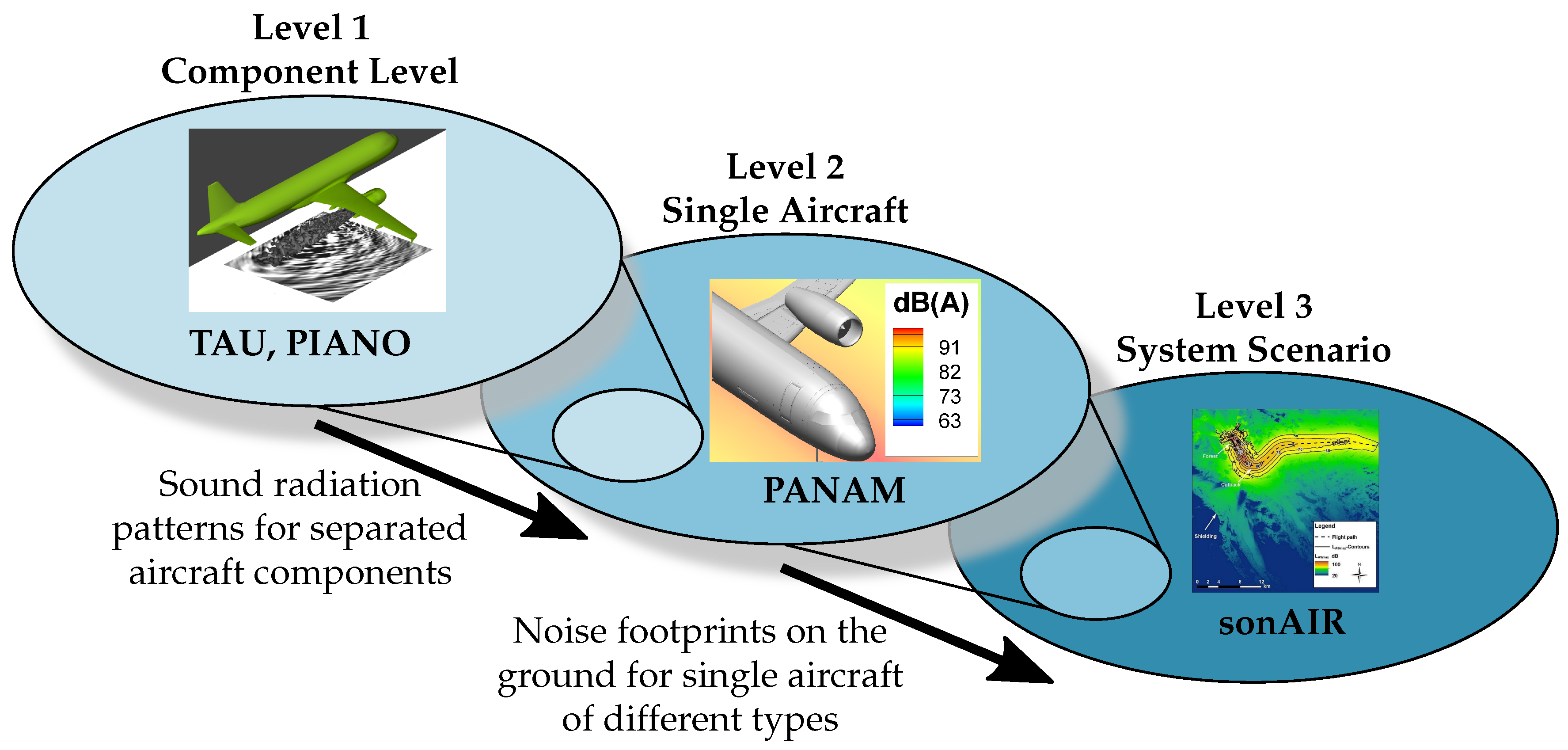
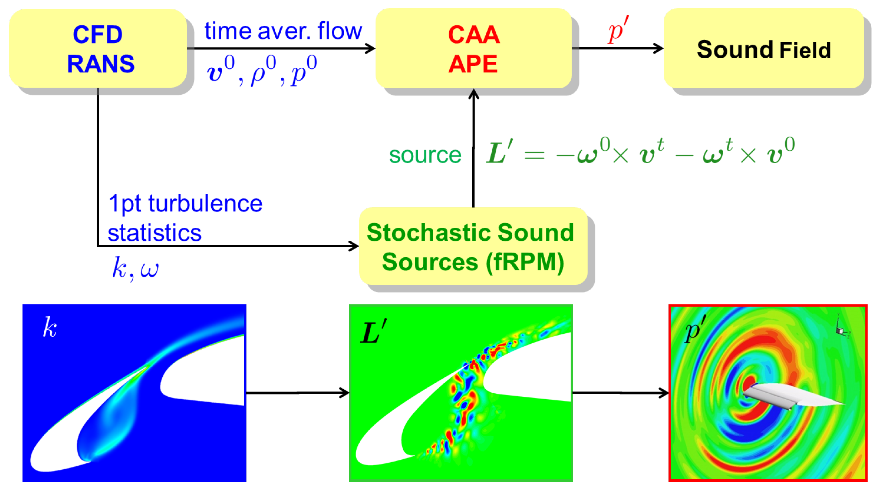
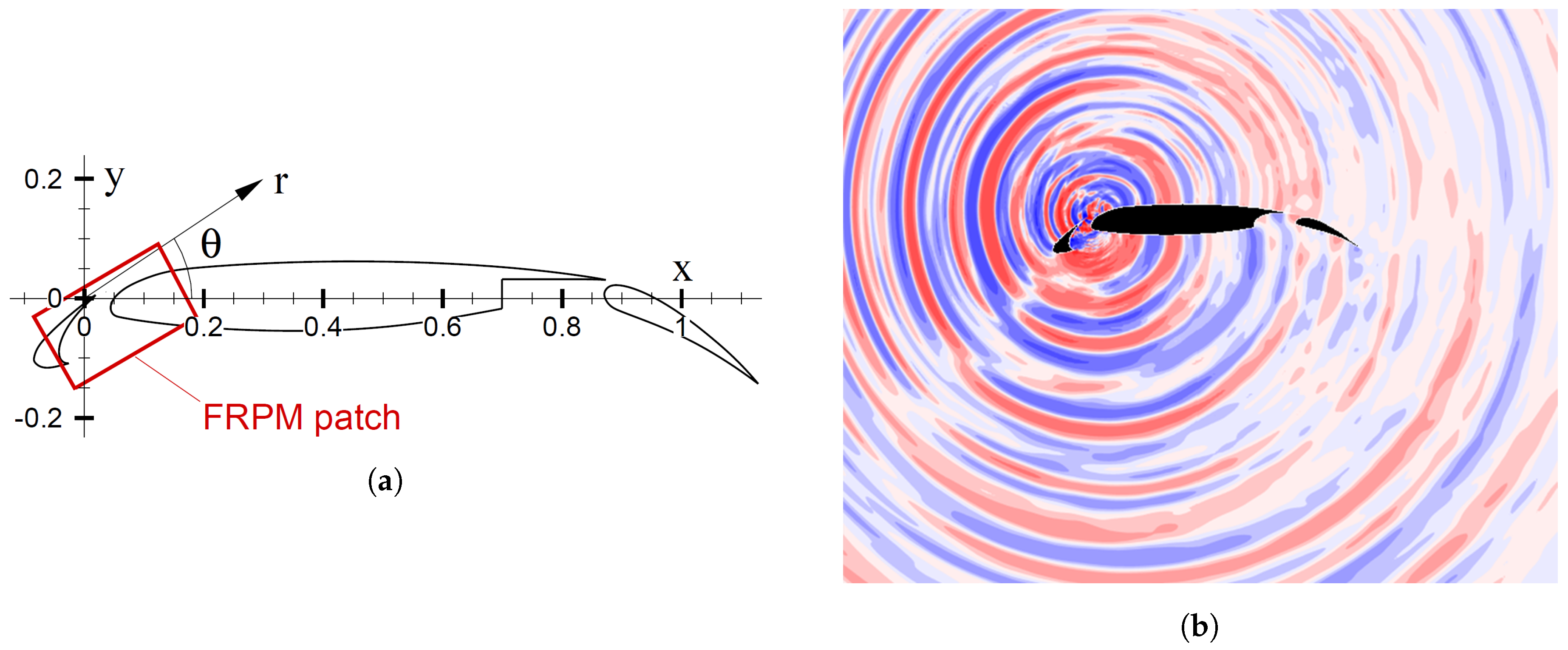
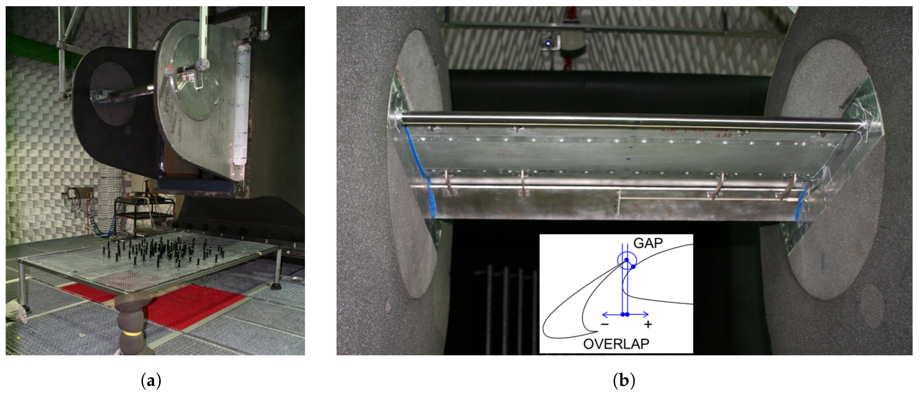
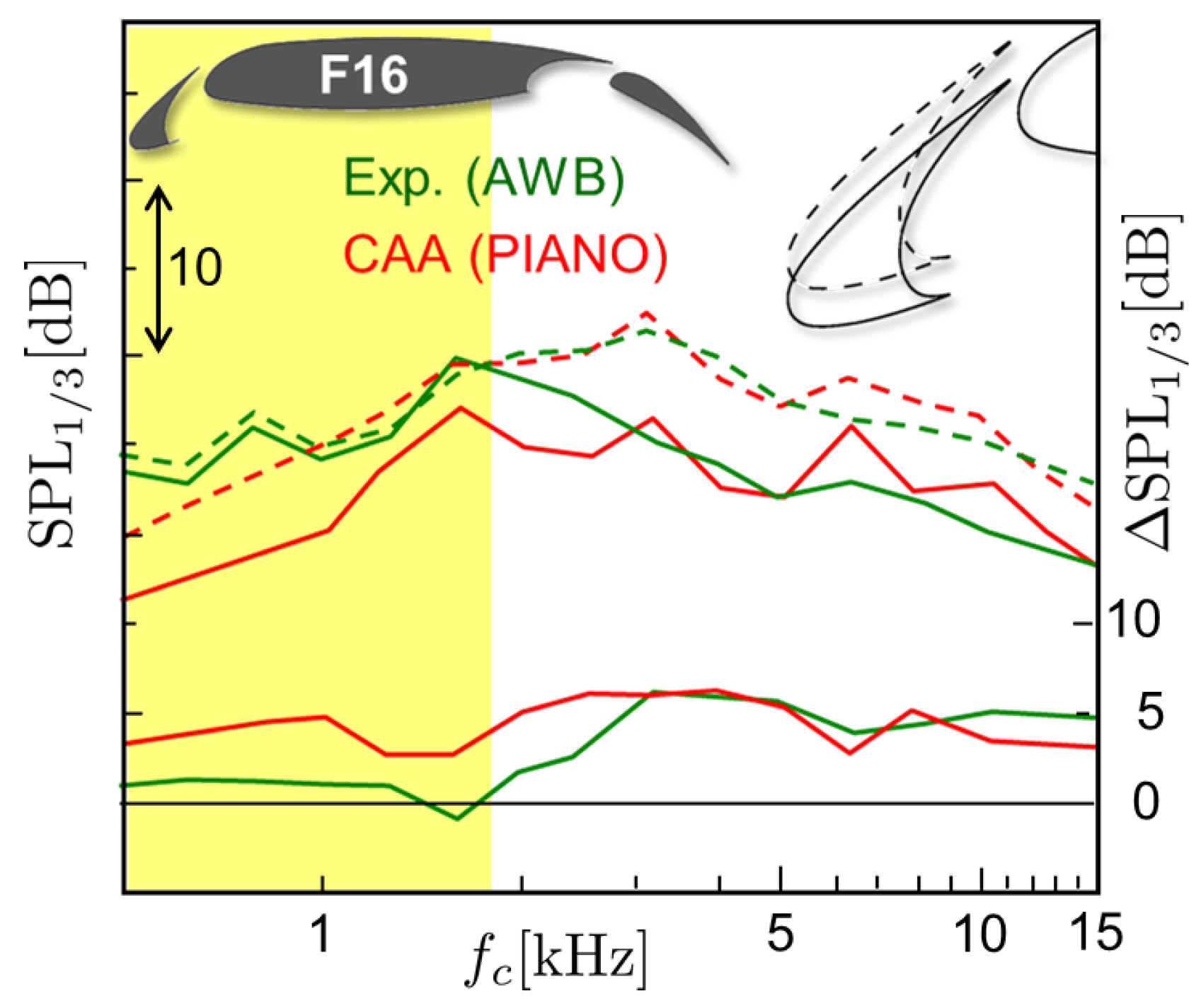
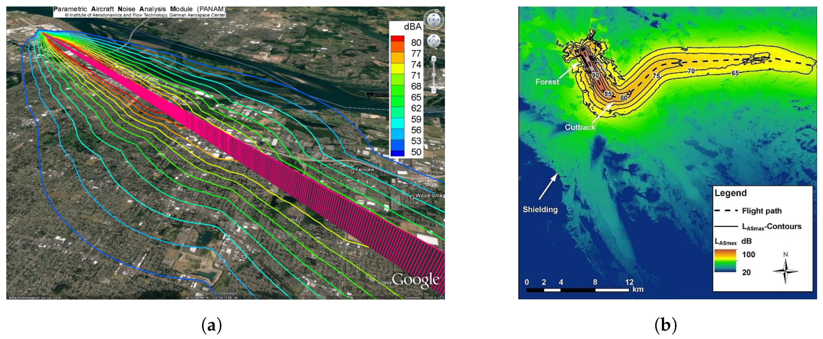
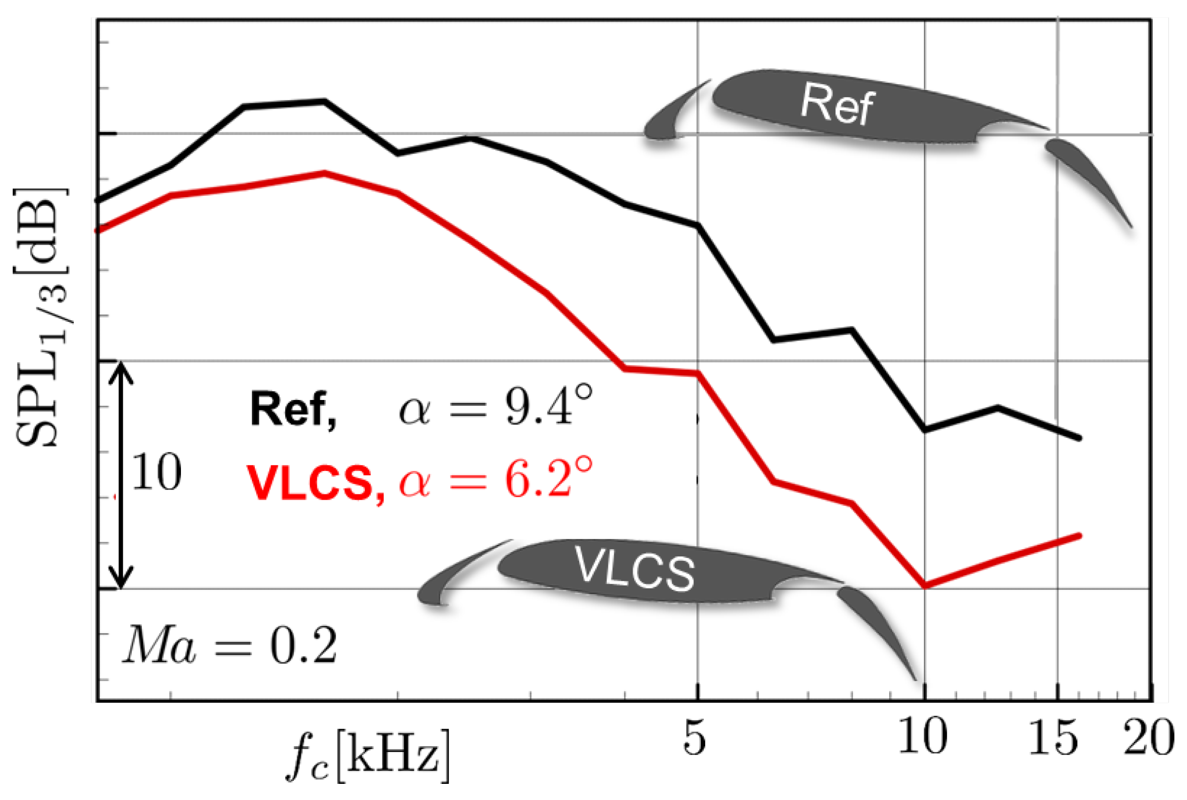
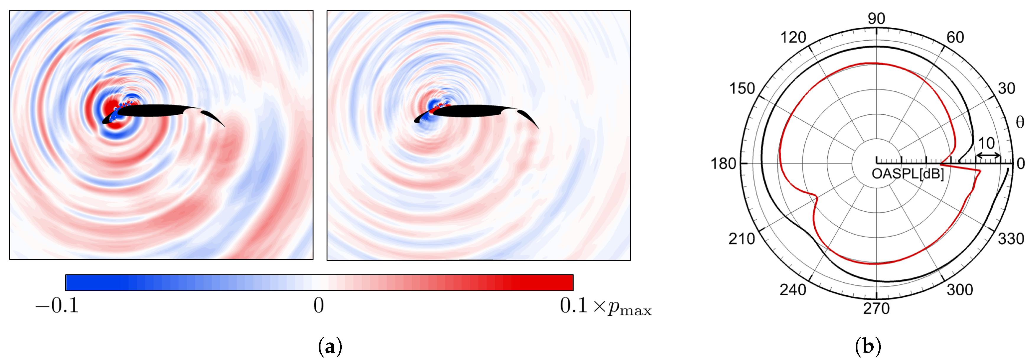
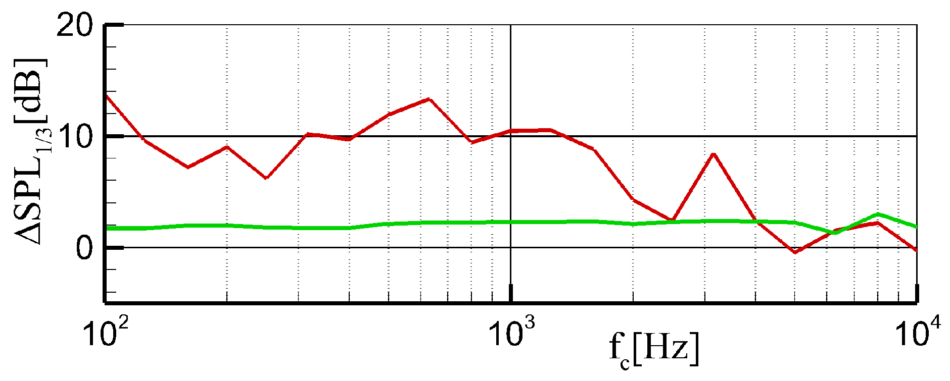
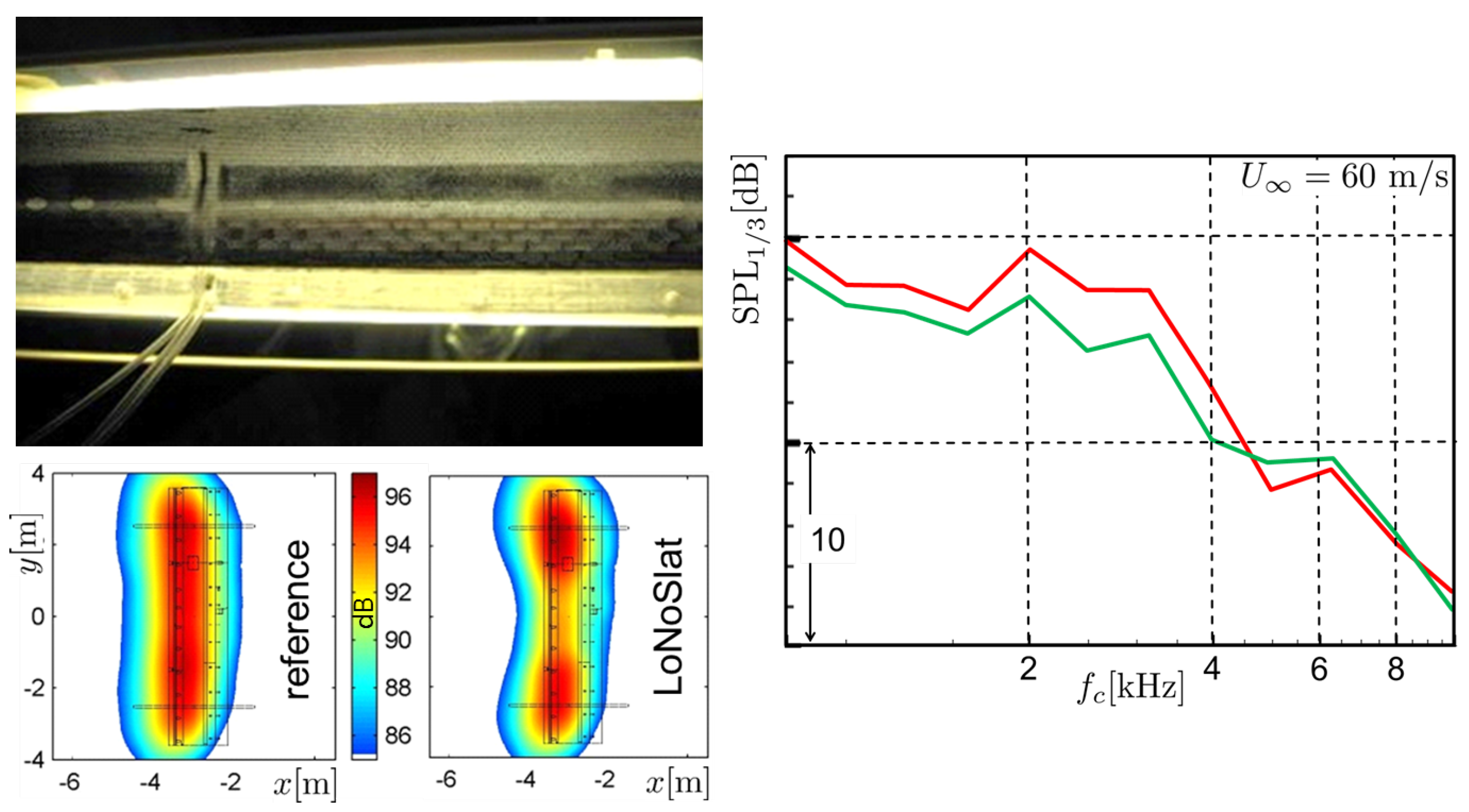
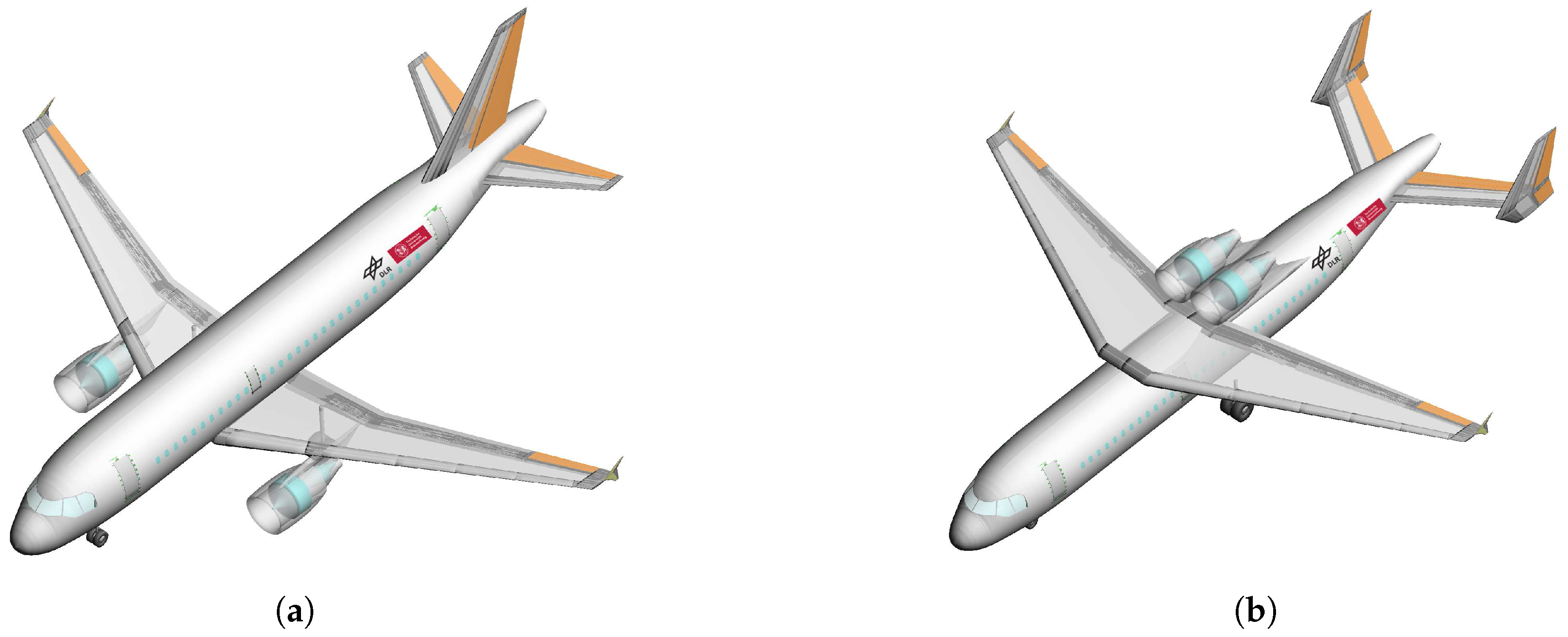
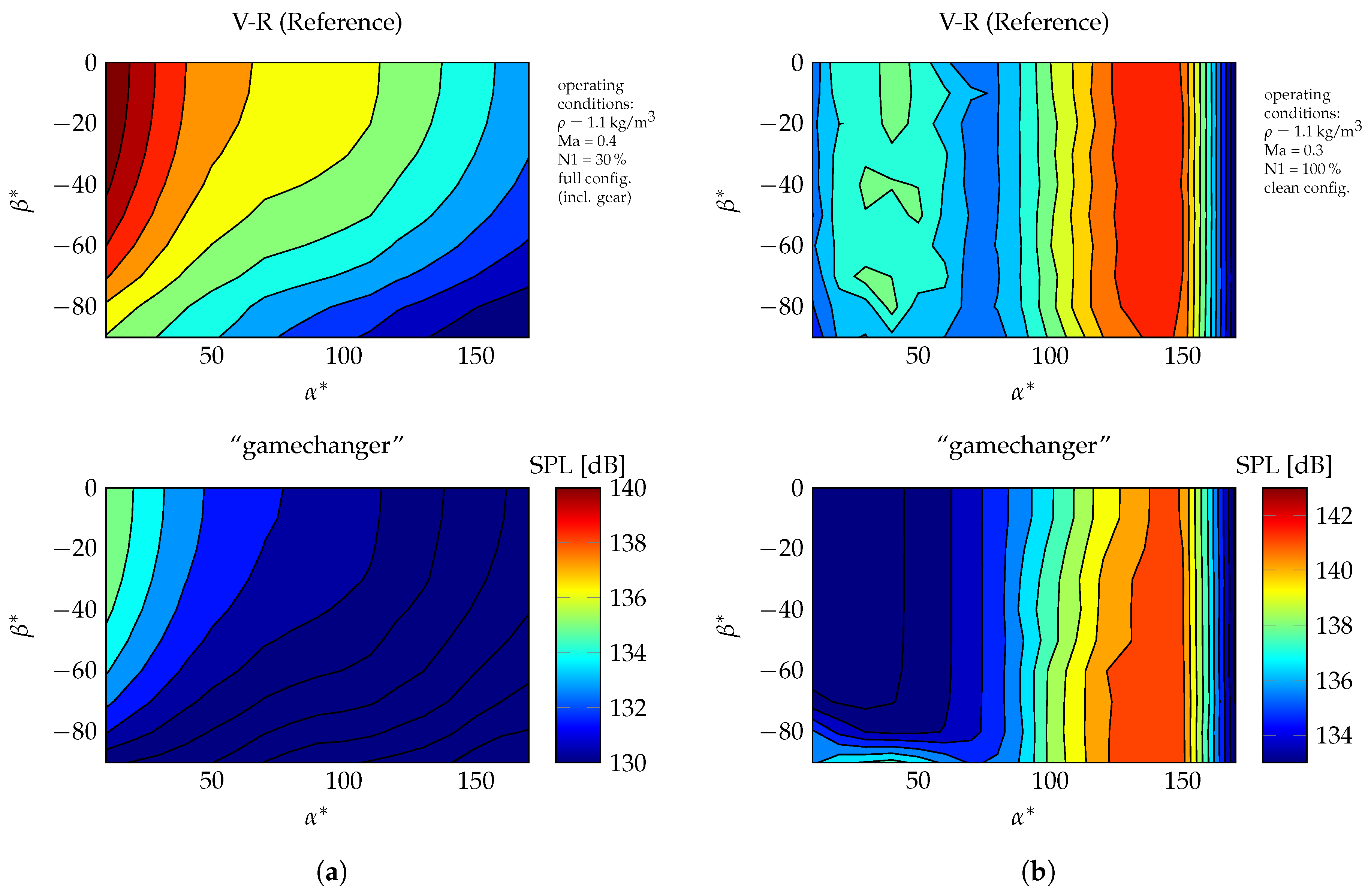
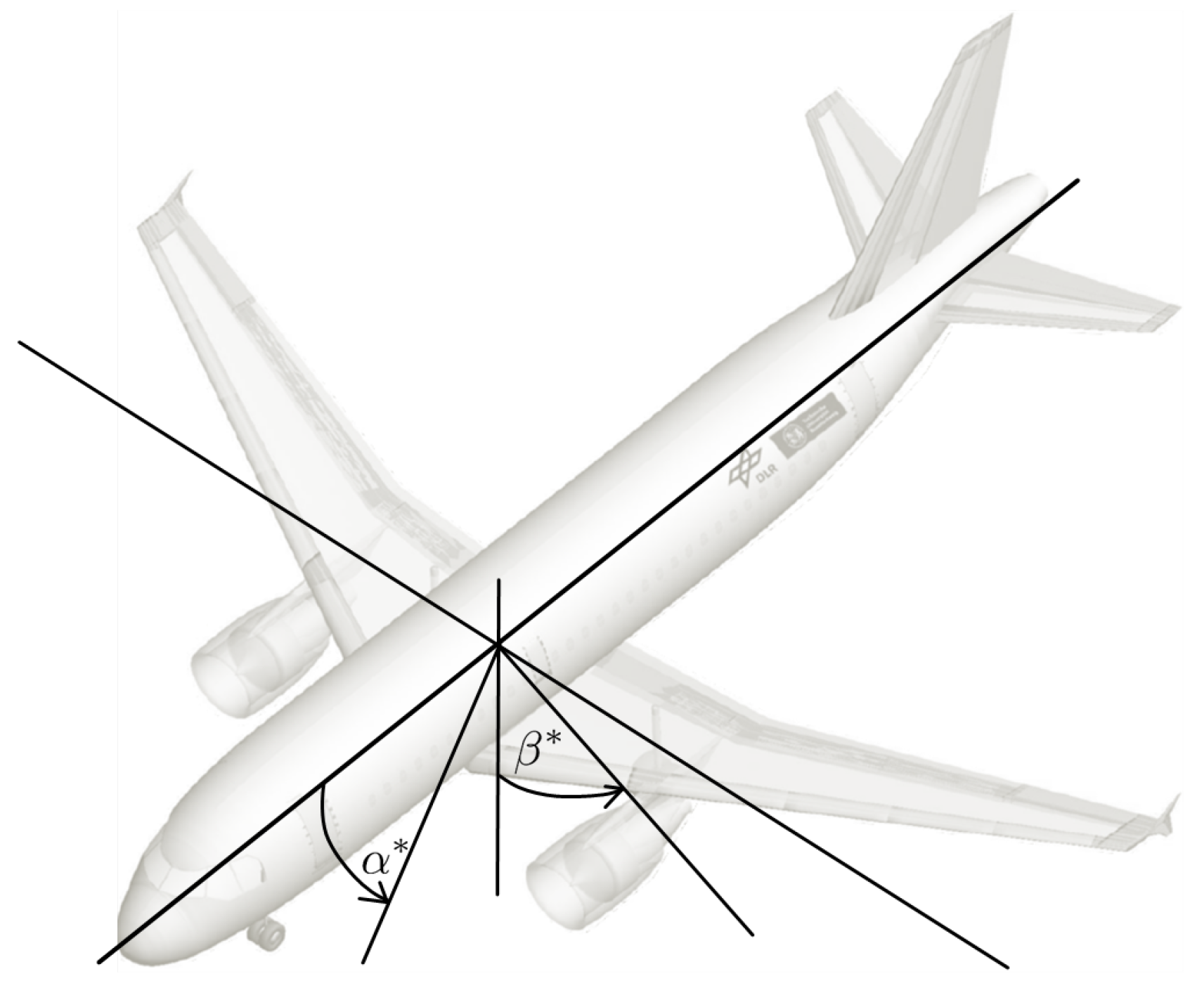
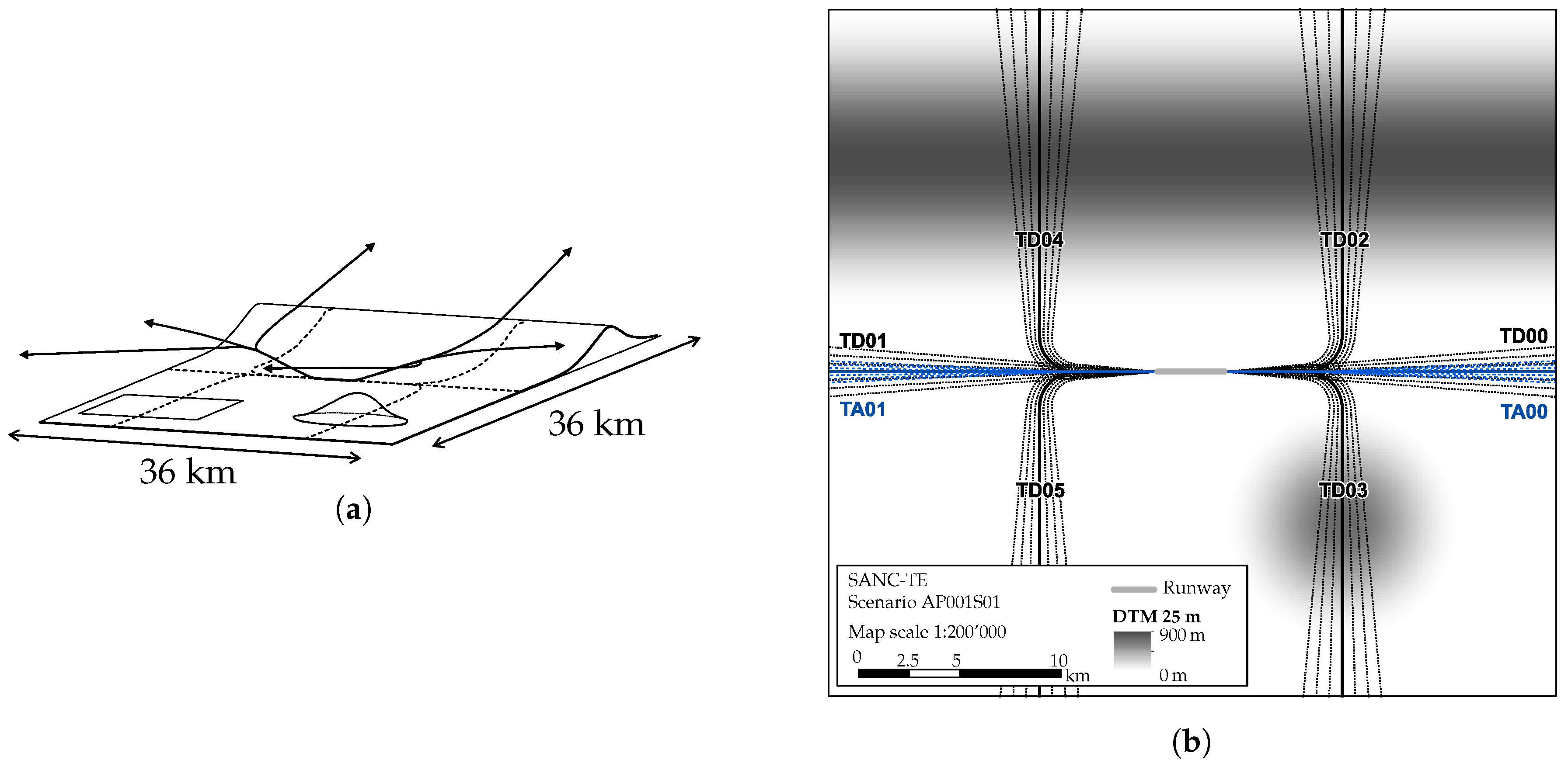
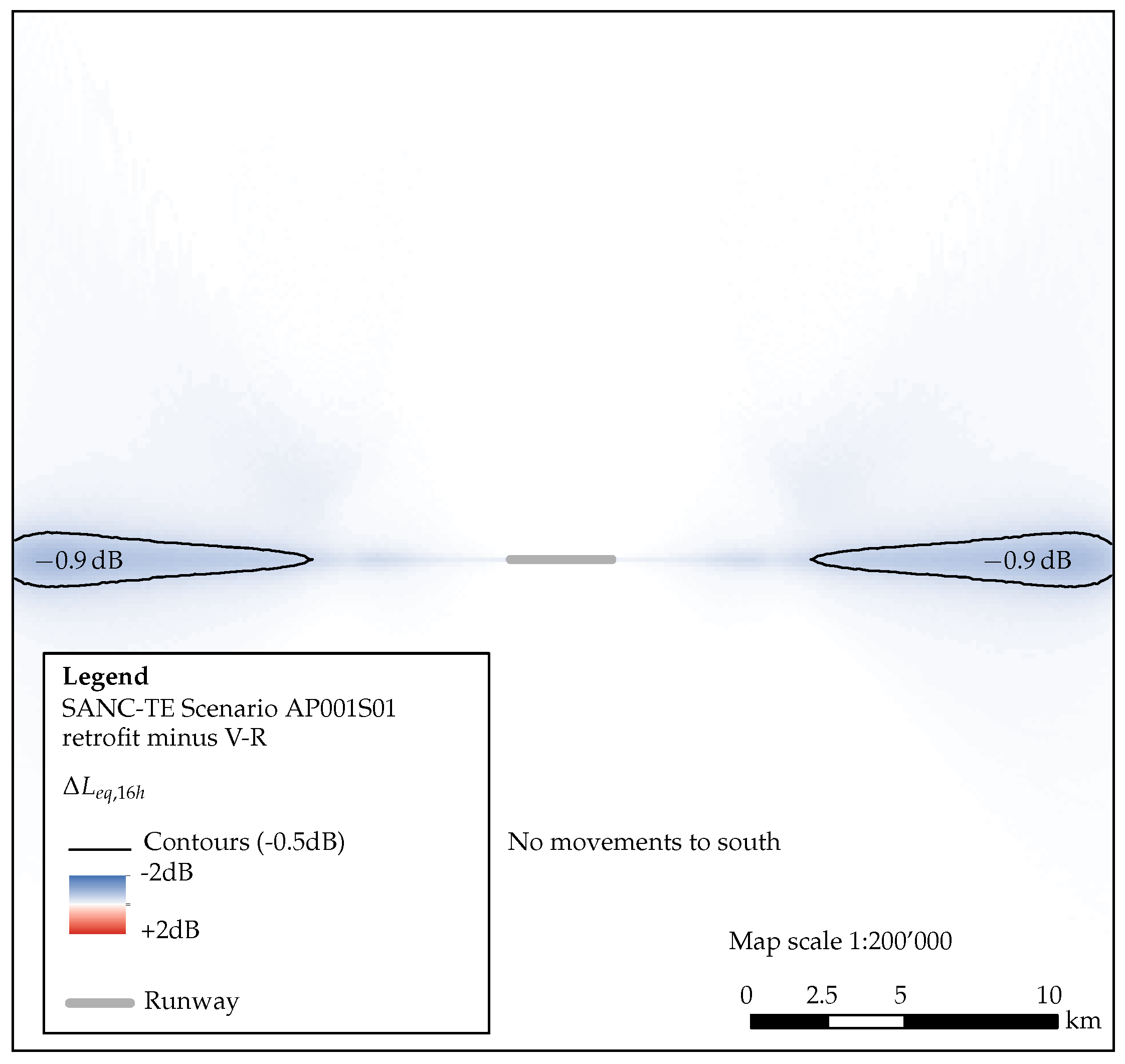
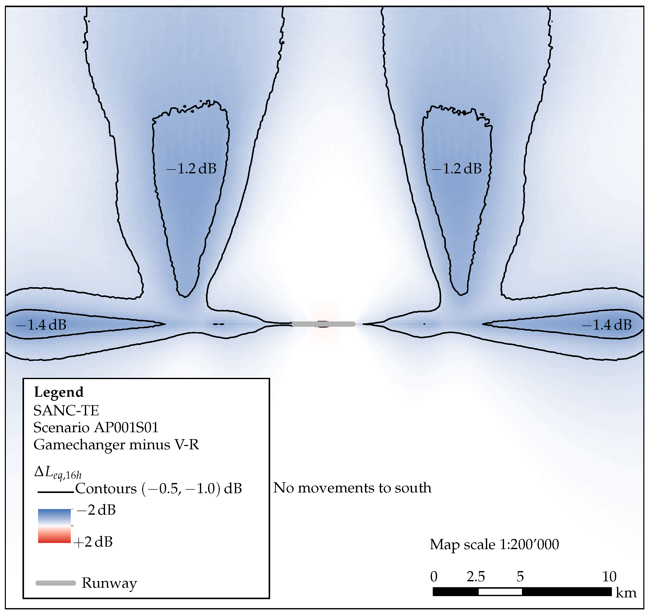
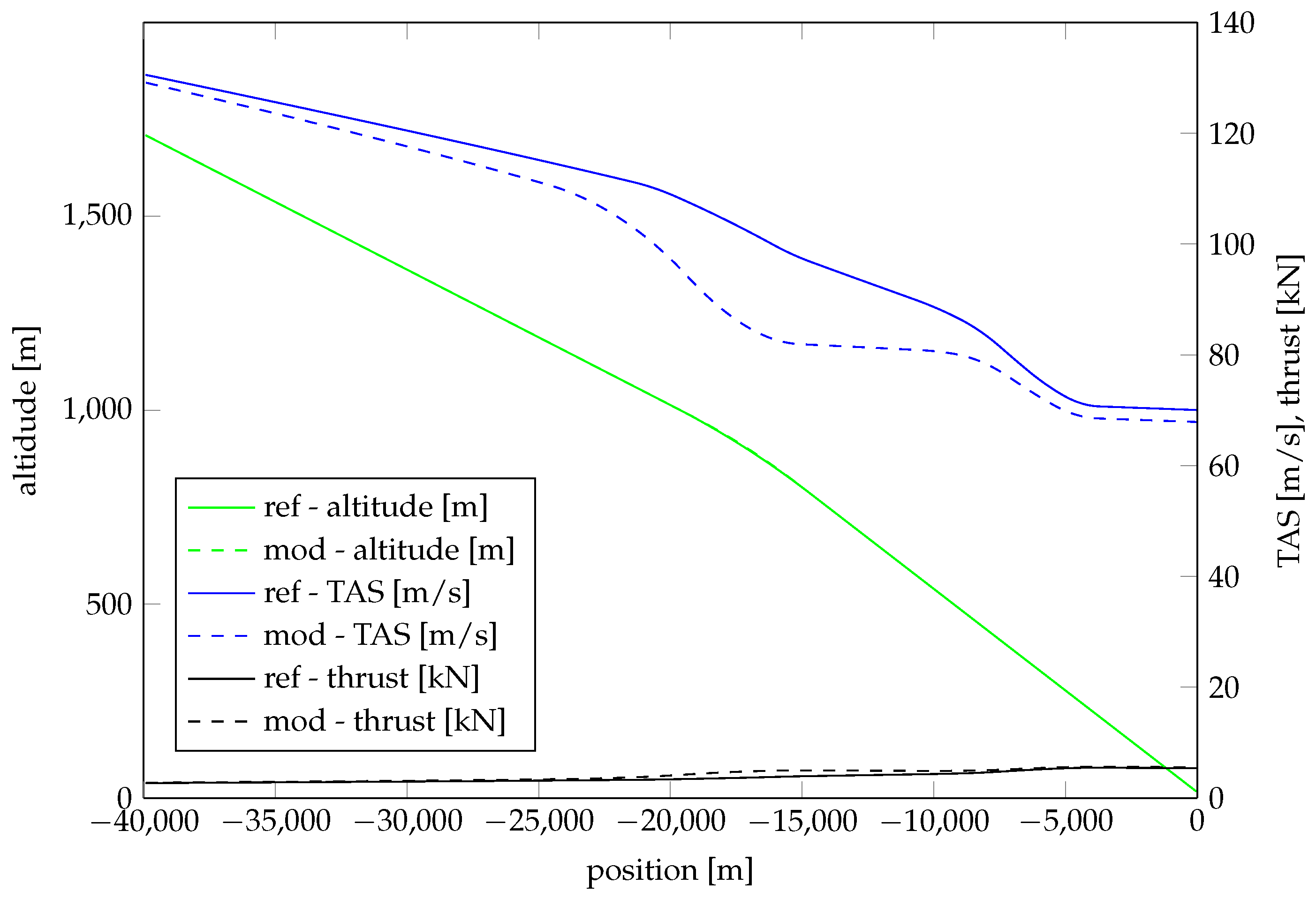
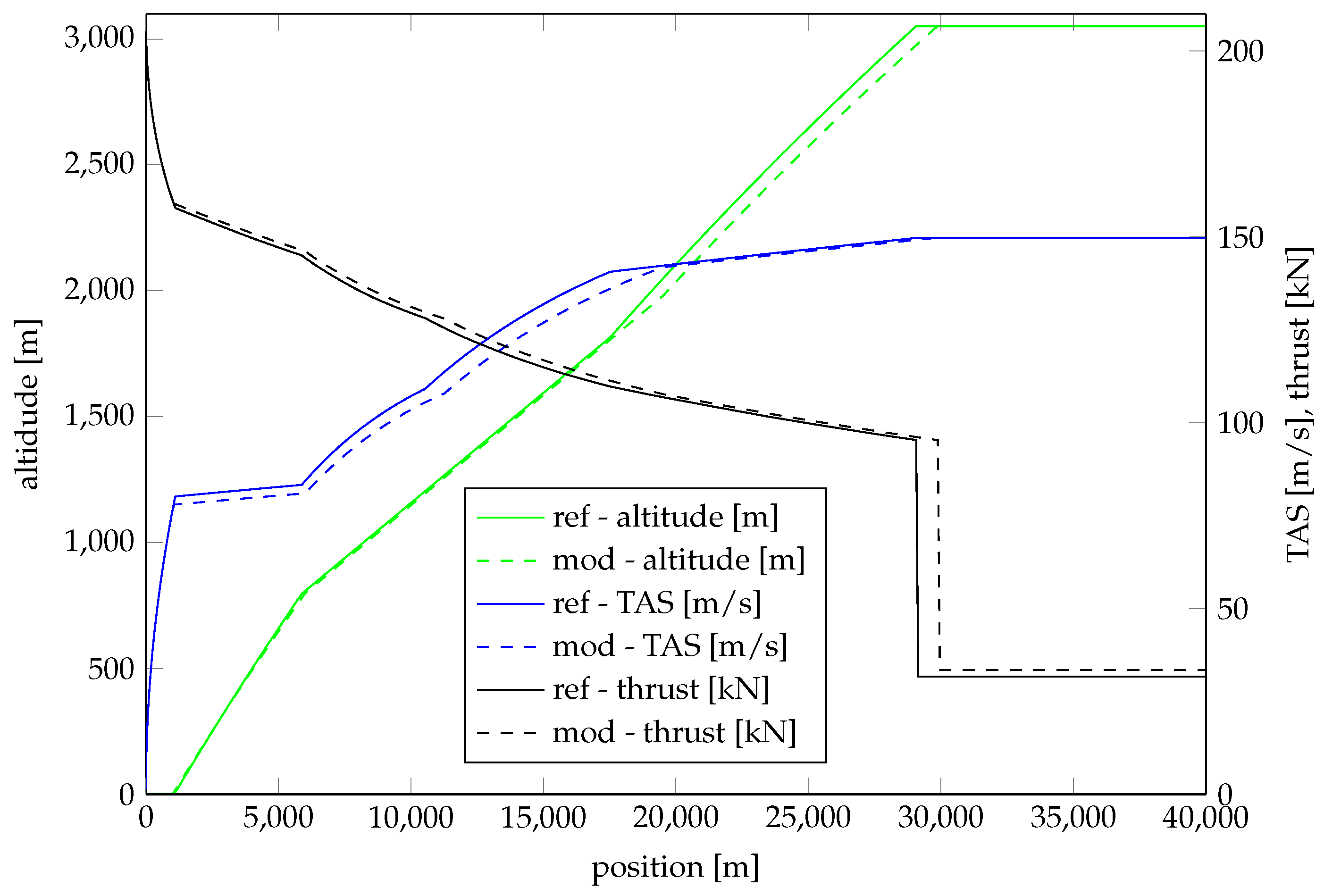
Table 1.
Swiss Aircraft Noise Calculation Test Environment (SANC-TE) aircraft types and number of yearly movements of the SANC-TE scenario AP001S01. The aircraft type A320 was substituted by the three aircraft concepts V-R, “retrofit” and “gamechanger”.
Table 1.
Swiss Aircraft Noise Calculation Test Environment (SANC-TE) aircraft types and number of yearly movements of the SANC-TE scenario AP001S01. The aircraft type A320 was substituted by the three aircraft concepts V-R, “retrofit” and “gamechanger”.
| Description | ICAO | TD00 | TD01 | TD02 | TD03 | TD04 | TD05 | TA00 | TA01 | Total |
|---|---|---|---|---|---|---|---|---|---|---|
| Airbus A320 | A320 | 1921 | 5763 | 3842 | 0 | 11,526 | 0 | 5763 | 17,289 | 46,104 |
| ATR42 (all series) | AT43 | 961 | 2881 | 0 | 1921 | 0 | 5763 | 2881 | 8645 | 23,052 |
| Boeing 747-400 | B744 | 192 | 576 | 384 | 0 | 1153 | 0 | 576 | 1729 | 4611 |
| Boeing 767-300 | B763 | 384 | 1153 | 769 | 0 | 2305 | 0 | 1153 | 3458 | 9221 |
| Cessna 550 Citation II | C550 | 961 | 2881 | 0 | 1921 | 0 | 5763 | 2881 | 8645 | 23,052 |
| Fokker 70 | F70 | 961 | 2881 | 0 | 1921 | 0 | 5763 | 2881 | 8645 | 23,052 |
| McDonnell Douglas MD-80/81/82 | MD81 | 1921 | 5763 | 0 | 3842 | 0 | 11,526 | 5763 | 17,289 | 46,104 |
| Total | 7300 | 21,899 | 4995 | 9604 | 14,984 | 28,815 | 21,899 | 65,701 | 175,198 |
© 2018 by the authors. Licensee MDPI, Basel, Switzerland. This article is an open access article distributed under the terms and conditions of the Creative Commons Attribution (CC BY) license (http://creativecommons.org/licenses/by/4.0/).
Share and Cite
MDPI and ACS Style
Delfs, J.; Bertsch, L.; Zellmann, C.; Rossian, L.; Kian Far, E.; Ring, T.; Langer, S.C. Aircraft Noise Assessment—From Single Components to Large Scenarios. Energies 2018, 11, 429. https://doi.org/10.3390/en11020429
AMA Style
Delfs J, Bertsch L, Zellmann C, Rossian L, Kian Far E, Ring T, Langer SC. Aircraft Noise Assessment—From Single Components to Large Scenarios. Energies. 2018; 11(2):429. https://doi.org/10.3390/en11020429
Chicago/Turabian StyleDelfs, Jan, Lothar Bertsch, Christoph Zellmann, Lennart Rossian, Ehsan Kian Far, Tobias Ring, and Sabine C. Langer. 2018. "Aircraft Noise Assessment—From Single Components to Large Scenarios" Energies 11, no. 2: 429. https://doi.org/10.3390/en11020429
Note that from the first issue of 2016, this journal uses article numbers instead of page numbers. See further details here.