A Hybrid BA-ELM Model Based on Factor Analysis and Similar-Day Approach for Short-Term Load Forecasting

Abstract

Accurate power-load forecasting for the safe and stable operation of a power system is of great significance. However, the random non-stationary electric-load time series which is affected by many factors hinders the improvement of prediction accuracy. In light of this, this paper innovatively combines factor analysis and similar-day thinking into a prediction model for short-term load forecasting. After factor analysis, the latent factors that affect load essentially are extracted from an original 22 influence factors. Then, considering the contribution rate of history load data, partial auto correlation function (PACF) is employed to further analyse the impact effect. In addition, ant colony clustering (ACC) is adopted to excavate the similar days that have common factors with the forecast day. Finally, an extreme learning machine (ELM), whose input weights and bias threshold are optimized by a bat algorithm (BA), hereafter referred as BA-ELM, is established to predict the electric load. A simulation experience using data deriving from Yangquan City shows its effectiveness and applicability, and the result demonstrates that the hybrid model can meet the needs of short-term electric load prediction.

1. Introduction

Short-term load forecasting is an important component of smart grids, which not only can achieve the goal of saving cost but also ensure a continuous flow of electricity supply [1]. Moreover, against the background of energy-saving and emission-reduction, accurate short-term load prediction plays an important role in avoiding a waste of resources in the process of power dispatch. Nevertheless, it should be noted that the inherent irregularity and linear independence of the loading data present a negative effect on the exact power load prediction.

Since the 1950s, short-term load forecasting has been attracting considerable attention from scholars. Generally speaking, the methods for load forecasting can be classified into two categories: traditional mathematical statistical methods and approaches which are based on artificial intelligence. The conventional methods like regression analysis [2,3] and time series [4] are mainly based on mathematical statistic models such as the vector auto-regression model (VAR) and auto-regressive moving average model (ARMA). With the development of science and technology, the shortcomings of statistical models, such as the effect of regression analysis based on historical data that will be weakened with the extension of time or the results of time-series prediction that are not ideal when the stochastic factors are large, are beginning to appear and are criticized by researchers for their low non-linear fitting capability.

Owing to the characteristic of strong self-learning, self-adapting ability and non-linearity, artificial intelligence methods such as back propagation neural networks (BPNN), support vector machine (SVM) as well as the least squares support vector machine (LSSVM) etc. have obtained greater attention and have had a wide application in the field of power load forecasting during the last decades [5,6]. Park [7] and his partners first used the artificial neural network in electricity forecasting. The experimental results demonstrated the higher fitting accuracy of the artificial neural network (ANNs) compared with the fundamental methods. Hernandez et al. [8] successfully presented a short-term electric load forecast architectural model based on ANNs and the results highlighted the simplicity of the proposed model. Yu and Xu [9] proposed a combinational approach for short-term gas-load forecasting including the improved BPNN and the real-coded genetic algorithm which is employed for the parameter optimization of the prediction model, and the simulation illustrated its superiority through the comparisons of several different combinational algorithms. Hu et al. [10] put forward a generalized regression neural network (GRNN) optimized by the decreasing step size fruit fly optimization algorithm to predict the short-term power load, and the proposed model showed a better performance with a stronger fitting ability and higher accuracy in comparison with traditional BPNN.

Yet, the inherent feature of BPNN may cause low efficiency and local optimal. Furthermore, the selection of the number of BPNN hidden nodes depends on trial and error. As a consequence, it is difficult to obtain the optimal network. On the basis of structural risk, empirical risk and vapnik–chervonenkis (VC) dimension bound minimization principle, the support vector machine (SVM) showed a smaller practical risk and presented a better performance in general [11]. Zhao and Wang [12] successfully conducted a SVM for short-term load forecasting, and the results demonstrated the excellence of the forecasting accuracy as well as computing speed. Considering the difficulty of the parameter determination that appeared in SVM, the least squares support vector machine (LSSVM) was put forward as an extension, which can transform the second optimal inequality constraints problem in original space into an equality constraints’ linear system in feature space through non-linear mapping and further improve the speed and accuracy of the prediction [13]. Nevertheless, how to set the kernel parameter and penalty factor of LSSVM scientifically is still a problem to be solved.

Huang et al. [14] proposed a new single-hidden layer feed forward neural network and named it as the extreme learning machine (ELM) in 2009, in which one can randomly choose hidden nodes and then analytically determine the output weights of single-hidden layer feed-forward neural network (SLFNs). The extreme learning machine tends to have better scalability and achieve similar (for regression and binary class cases) or much better (for multi-class cases) generalization performance at much faster learning speed (up to thousands of times) than the traditional SVM and LSSVM [15]. However, it is worth noting that the input weights matrix and hidden layer bias assigned randomly may affect the generalization ability of the ELM. Consequently, employing an optimization algorithm so as to obtain the best parameters of both the weight of input layer and the bias of the hidden layer is vital and necessary. The bat algorithm (BA), acknowledged as a new meta-heuristic method, can control the mutual conversion between local search and global search dynamically and performs better convergence [16]. Because of the excellent performance of local search and global search in comparison with existing algorithms like the genetic algorithm (GA) and particle swarm optimization algorithm (PSO), researchers and scholars have applied BA in diverse optimization problems extensively [17,18,19]. Thus, this paper adopted the bat algorithm to obtain the input weight matrix and the hidden layer bias matrix of ELM corresponding to the minimum training error, which can not only maximize the merit of BA’s global and local search capability and ELM’s fast learning speed, but also overcome the inherent instability of ELM.

The importance of forecasting methods is self-evident, yet the analysis and processing of the original load data also cannot be ignored. Some predecessors have supposed historical load and weather as the most influential factors in their research [20,21,22]. However, selecting the historical load data scientifically or not can cause a strong impact on the accuracy of prediction. In addition, there are still many other external weather factors that may also potentially influence the power load. Only considering the temperature as the input variable may be not enough [23,24,25], and other meteorological factors such as humidity, visibility and air pressure etc. also should be taken into consideration. Besides, it is necessary to analyze and pretreat the influence factors on the premise of considering the influence factors synthetically so as to achieve the goal of improving the generalization ability and the precision of the prediction model. Therefore, this paper applied factor analysis (FA) and the similar-day approach (SDA) for input data pre-processing, where the former is utilized to extract the latent factors that essentially affect the load and the SDA is adopted to excavate the similar days that have common factors with the forecast day.

To sum up, the load forecasting process of the ELM optimized by the bat algorithm can be elaborated in four steps. Firstly, based on 22 original influence factors, factor analysis is adopted to extract the latent factors which essentially affect load. To further explore the relationship between historical load and current load, a partial auto correlation function (PCAF) is applied to demonstrate the significance of previous data. Then, in accordance with the latent factors and the loads of each day, ant colony clustering is used to divide the load to different clusters.

The rest of the paper is organized as follows: Section 2 gives a brief description about the material and methods, including bat algorithm (BA), extreme learning machine (ELM), ant colony clustering algorithm (ACC) as well as the framework of the whole model. Data analysis and processing are considered in Section 3 and Section 4 which present an empirical analysis of the power load forecasting. Finally, conclusions are drawn in Section 5.

2. Methodology

2.1. Bat Algorithm

Based on the echolocation of micro-bats, Yang [26] proposed a new meta-heuristic method and called it the bat algorithm, one that combines the advantages both the genetic algorithm and particle swarm optimization with the superiority of parallelism, quick convergence, distribution and less parameter adjustment. In the d dimensions of search space during the global search, the bat i has the position of ${\mathrm{x}}_{\mathrm{i}}^{\mathrm{t}}$, and velocity ${\mathrm{v}}_{\mathrm{i}}^{\mathrm{t}}$ at the time of t, whose position and velocity will be updated as Equations (1) and (2), respectively:

$${\mathrm{x}}_{\mathrm{i}}^{\mathrm{t}+1}={\mathrm{x}}_{\mathrm{i}}^{\mathrm{t}}+{\mathrm{v}}_{\mathrm{i}}^{\mathrm{t}+1};$$

(1)

$${\mathrm{v}}_{\mathrm{i}}^{\mathrm{t}+1}={\mathrm{v}}_{\mathrm{i}}^{\mathrm{t}}+\left({\mathrm{x}}_{\mathrm{i}}^{\mathrm{t}}-{\mathrm{x}}^{^}\right)·{\mathrm{F}}_{\mathrm{i}}$$

(2)

where x^{^} is the current global optimal solution; and F_i is the sonic wave frequency which can be seen in Equation (3):

$${\mathrm{F}}_{\mathrm{i}}={\mathrm{F}}_{\min }+\left({\mathrm{F}}_{\max }-{\mathrm{F}}_{\min }\right)\mathsf{\beta }$$

(3)

where β is a random number within [0, 1]; F_max and F_min are the max and min sonic wave frequency of the bat I. In the process of flying, each initial bat is assigned one random frequency in line with [F_min, F_max].

In local search, once a solution is selected in the current global optimal solution, each bat would produce a new alternative solution in the mode of random walk according to Equation (4):

$${\mathrm{x}}_{\mathrm{n}}\left(\mathrm{i}\right)={\mathrm{x}}_0+{\mathsf{\mu }\mathrm{A}}^{\mathrm{t}}$$

(4)

where ${\mathrm{x}}_0$ is a solution that is chosen in current optimal disaggregation randomly; ${\mathrm{A}}^{\mathrm{t}}$ is the average volume of the current bat population; and $\mathsf{\mu }$ is a D dimensional vector within in [−1, 1].

The balance of bats is controlled by the impulse volume $\mathrm{A}\left(\mathrm{i}\right)$ and impulse emission rate $\mathrm{R}\left(\mathrm{i}\right)$. Once the bat locks the prey, the volume A(i) will be reduced and the emission rate R(i) will be increased at the same time. The update of $\mathrm{A}\left(\mathrm{i}\right)$ and $\mathrm{R}\left(\mathrm{i}\right)$ are expressed as Equations (5) and (6), respectively:

$${\mathrm{A}}^{\mathrm{t}+1}\left(\mathrm{i}\right)={\mathsf{\gamma }\mathrm{A}}^{\mathrm{t}}\left(\mathrm{i}\right)$$

(5)

$${\mathrm{R}}^{\mathrm{t}+1}={\mathrm{R}}^0\left(\mathrm{i}\right)·(1-{\mathrm{e}}^{-\mathsf{\theta }\mathrm{t}})$$

(6)

where $\mathsf{\gamma }$ and $\mathsf{\theta }$ are both constants that $\mathsf{\gamma }$ is within [0, 1] and $\mathsf{\theta }>0$. This paper set the two parameters as $\mathsf{\gamma }=\mathsf{\theta }=0.9.$ The basic steps of the standard bat algorithm can be summarized as the pseudo code seen in the following:

Bat algorithm.

1: Initialize the location of bat populations xi (i = 1, 2, 3, …, n) and velocity vi

2: Initialize frequency Fi pulse emission rate Ri and loudness Ai

3: While (t < the maximum number of iterations)

4:   Generate new solutions by adjusting the frequency

5:   Generate new velocity and location

6:   If (rand >Ri)

7:   Select a solution among best solutions

8:   Generate new local solution around the selected best solution

9: End if

10:   Get a new solution through flying randomly

11: If (rand < Ai & f(xi) < f(x*))

12:   Accept the new solution

13:   Increase ri and decrease Ai

14: End if

15:   Rank the bats and find the current best x*.

16: End

2.2. Extreme Learning Machine

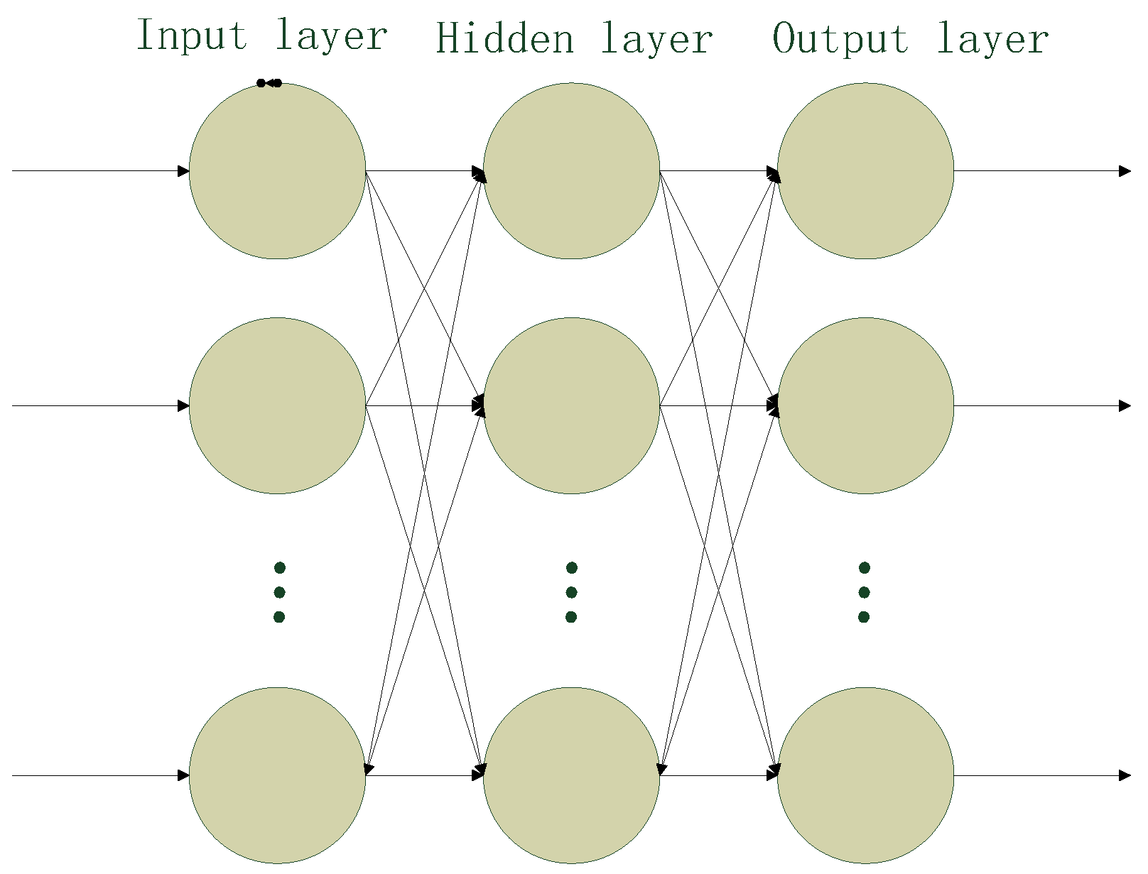
After setting the input weights and hidden layer biases randomly, the output weights of the ELM can be analytically determined by solving a linear system in accordance with the thinking of the Moore–Penrose (MP) generalized inverse. The only two parameters needed to be assigned allow the extreme learning machine to generate the input weights matrix and hidden layer biases automatically at fast running speed. Consequently, the extreme learning machine expresses the advantages of a fast learning speed, small training error and strong generalization ability compared with the traditional neural networks in solving non-linearity problems [27]. The concrete framework of ELM is shown in Figure 1 and the computational steps of the standard ELM can be illustrated as follows:

The connection weights both between input layer and hidden layer and between hidden layer and output layer as well as the hidden layer neuron threshold are shown in the following:

$$\mathsf{\omega }={\left[{\mathsf{\omega }}_{\mathrm{i}1},{\mathsf{\omega }}_{\mathrm{i}2},\cdots ,{\mathsf{\omega }}_{\mathrm{in}}\right]}_{\mathrm{L}\times \mathrm{n}}$$

(7)

where $\mathsf{\omega }$ is the connection weights between input layer and hidden layer; $\mathrm{n}$ is the input layer neuron number, and $\mathrm{L}$ is the hidden layer neuron number, and,

$$\mathsf{\beta }={\left[{\mathsf{\beta }}_{\mathrm{i}1},{\mathsf{\beta }}_{\mathrm{i}2},\cdots ,{\mathsf{\beta }}_{\mathrm{im}}\right]}_{\mathrm{L}\times \mathrm{m}}$$

(8)

where $\mathsf{\beta }$ is the connection weights between hidden layer and output layer and $\mathrm{m}$ is the output layer neuron number, and,

$$\mathrm{X}={\left[{\mathrm{x}}_{\mathrm{i}1},{\mathrm{x}}_{\mathrm{i}2},\cdots ,{\mathrm{x}}_{\mathrm{iQ}}\right]}_{\mathrm{n}\times \mathrm{Q}}$$

(9)

$$\mathrm{Y}={\left[{\mathrm{y}}_{\mathrm{i}1},{\mathrm{y}}_{\mathrm{i}2},\cdots ,{\mathrm{y}}_{\mathrm{iQ}}\right]}_{\mathrm{m}\times \mathrm{Q}}$$

(10)

where $\mathrm{X}$ is the input vector and $\mathrm{Y}$ is the corresponding output vector, and,

$$\mathrm{H}=\left[\begin{array}{cccc}\mathrm{g}\left({\mathsf{\omega }}_1{\mathrm{x}}_1+{\mathrm{b}}_1\right)& \mathrm{g}\left({\mathsf{\omega }}_2{\mathrm{x}}_1+{\mathrm{b}}_2\right)& \cdots & \mathrm{g}\left({\mathsf{\omega }}_{\mathrm{l}}{\mathrm{x}}_1+{\mathrm{b}}_{\mathrm{l}}\right)\\ \mathrm{g}\left({\mathsf{\omega }}_1{\mathrm{x}}_2+{\mathrm{b}}_1\right)& \mathrm{g}\left({\mathsf{\omega }}_2{\mathrm{x}}_2+{\mathrm{b}}_2\right)& \cdots & \mathrm{g}\left({\mathsf{\omega }}_1{\mathrm{x}}_2+{\mathrm{b}}_1\right)\\ ⋮& ⋮& & ⋮\\ \mathrm{g}\left({\mathsf{\omega }}_1{\mathrm{x}}_{\mathrm{Q}}+{\mathrm{b}}_1\right)& \mathrm{g}\left({\mathsf{\omega }}_2{\mathrm{x}}_{\mathrm{Q}}+{\mathrm{b}}_2\right)& \cdots & \mathrm{g}\left({\mathsf{\omega }}_{\mathrm{l}}{\mathrm{x}}_{\mathrm{Q}}+{\mathrm{b}}_{\mathrm{l}}\right)\end{array}\right]$$

(11)

where H is the hidden layer output matrix, b is the bias which is generated randomly in the process of network initialization, and g(x) is the activation function of the ELM.

2.3. Ant Colony Clustering Algorithm

When processing the large number of samples, the traditional clustering learning algorithm often has the disadvantages of slow clustering speed, falling easily into local optimal, and it is difficult to obtain the optimal clustering result. At the same time, the clustering algorithm involves the selection of the number of clustering K, which directly affects the clustering result. Using ant colony clustering to pre-process the load samples can reduce the number of input samples on the premise of including all sample features, and also can effectively simplify the network structure and reduce the calculation effort. The flowchart of the ant colony clustering algorithm is shown in Figure 2.

2.4. Introduction of Factor Analysis-Ant Colony Clustering-Bat Algorithm-Extreme Learning Machine (FA-ACC-BA-ELM) Model

Since the ELM has less ability to respond to samples of the training set, its generalization ability is insufficient. So we propose BA-ELM. In this paper, the flowchart of the factor analysis-similar day-bat algorithm-extreme learning machine (FA-SD-BA-ELM) model is shown in Figure 3. As discussed in part 1, auto correlation and the partial correlation function (PACF) are executed to analyze the inner relationships between the history loads. Based on the influencing factors of load, factor analysis (FA) is used for extracting input variables. According to the result of factors analysis and previous load, the ant colony clustering algorithm (ACC) is used to find historical days that have common factors similar to the forecast day. Part 2 is the bat optimization algorithm (BA) and part 3 is the forecasting of the extreme learning machine (ELM).

3. Data Analysis and Preprocessing

3.1. Selection of Influenced Indexes

Considering that the human activities are always disturbed by many external factors and then the power load is affected, some effective features are selected as factors. In this paper, the selection of factors is mainly based on four aspects:

(1)

The historical load. Generally speaking, the historical load impacts on the current load in short-term load forecasting. In this paper, the daily maximum load, daily minimum load, average daily load, peak average load of previous day, valley average load of previous day, average load of the day before, average load of ₂ days before, average load of 3 days before, average load of 4 days before, average load of ₅ days before and average load of 6 days before are taken into consideration.

(2)

The temperature. As people use temperature-adjusting devices to adapt to the temperature, in a previous study [23,24,25], temperature was considered as an essential input feature and the forecasting results were accurate enough. In this paper, the maximum temperature, the minimum temperature and the average temperature are selected as factors.

(3)

The weather condition. We mainly take into account the seasonal patterns, humidity, visibility, weather patterns, air pressure and wind speed. The four seasons are represented as 1, 2, 3 and 4 respectively. For different weather patterns, we set different weights: {sunny, cloudy, overcast, rainy} = {0, 1, 2, 3}.

(4)

The day type. In this aspect, the type of day and date are taken into consideration. The type of date means the days are divided into workdays (Monday–Friday), weekend (Saturday–Sunday), and holidays. The weights of three types of date are 0, 1 and 2 respectively. For the date, we set different weight: {Monday, Tuesday, Wednesday, Thursday, Friday, Saturday, Sunday} = {1, 2, 3, 4, 5, 6, 7}.

3.2. Factor Analysis

Originally proposed by British psychologist C.E. Spearman, factor analysis is the study of statistical techniques for extracting highly interrelated variables into one group, and each type of group becomes a factor that reflects most of the original information with fewer factors. Not only does factor analysis reduce indicators’ dimensions and improve the generalization of the model but also the common factors it elicited to portray and replace primitive variables can commendably mirror and explain the complicated relationship between variables, keeping data messages with essentially no less information. In this paper, factor analysis is used to extract factors that can reflect the most information of the original 22 influencing variables, whose result is shown in Table 2.

First of all,

Table 1. KMO and Barlett test of sphericity.

KMO	Value	0.740
Barlett test of sphericity	Approximate chi-square value	1525.304
	Degrees of freedom (Df.)	231
	Significance (Sig.)	0.000

gives the result of Kaiser-Meyer-Olkin (KMO) and the Barlett test of sphericity that can serve as a criteria to judge whether the data is suitable for the factor analysis. The statistic value more than 0.7 can illustrate the compatibility and the 0.74 obtained from the power load data confirms the correctness of factor analysis.

Table 2. Results of factor analysis.

Indicator	Variable	Load	Contribution Rate (%)
Factor 1	Minimum temperature	0.732	35.128
	Daily maximum load	0.714
	Daily minimum load	0.726
	Average daily load	0.870
	Season patterns	0.736
	Peak average load of previous day	0.922
	Valley average load of previous day	0.801
	Average load of the day before	0.917
	Average load of 2 days before	0.830
	Average load of 3 days before	0.695
Factor 2	Maximum temperature	−0.732	19.646
	Average temperature	−0.697
	Humidity	0.810
	Visibility	−0.724
	Weather patterns	0.724
	Average load of 4 days before	0.547
Factor 3	Type of date	0.622	10.514
	Average load of 5 days before	0.612
	Average load of 6 days before	0.609
Factor 4	Air pressure	0.563	7.746
Factor 5	Date	0.883	6.087
Factor 6	Wind speed	−0.533	5.313

shows six factors that are extracted from 22 original variables. The accumulative contribution rate at 84.434%, more than 80%, reflects that the new six factors can deliver the most information of the original indicators. It can be seen from Table 2 that factor 1 that mainly represents the history load accounts for the largest proportion at 35.128%. In addition, considering that the variables in factor 1 may not be sufficient on behalf of the historical load, the paper carried out a further analysis of the previous data by means of the correlation analysis which can be seen in part 3.2. Factor 2 which mainly represents meteorology element accounts for 19.646%, and the remaining four factors are 10.514%, 7.746%, 6.087%, and 5.313%, respectively.

3.3. The Analysis of Correlation

Additionally, this paper conducted a further analysis of the correlation between the amount of historical load and the target load from two different viewpoints so as to eliminate the internal correlation. On the one hand, the partial auto correlation function (PACF) was carried out throughout the overall power load to dig out the correlation between the target load and the previous load. On the other hand, the whole load data with the same time interval were also implemented by PACF individually to seek the relationship among the load with the same time. The results of partial auto correlation can be seen in Figure 4 and Figure 5, respectively.

For instance, under the confidence level of 90%, it can be seen from Figure 4 that the lags of the first 2 h are significant to the current data. That is to say, the loads of the first two hours are influential to the current load. As for Figure 5, it is known that only the first lag 1 is prominent to the current load data except the load of 00:00 (Lag 2). Consequently, it can be concluded that the four factors including the first two hours before 00:00 and the same time power load that occurred yesterday and the day before yesterday were selected as the input factors at the time of 00:00.

3.4. Clustering with Ant Colony Algorithm

Selecting the exogenous features as input directly may lead the prediction model to a slow convergence and to poor prediction accuracy. Thus, the paper employs the similar day load which is clustered by the ant colony clustering algorithm for the prediction so as to improve the forecasting accuracy. According to the load every day and the six factors extracted from 22 variables, the 60 days from 1 May 2013 to 30 June 2013 are named with numbers from 1 to 60 and are divided into four clusters by the ant colony algorithm. The parameters of the ACC algorithm can be seen in

Table 3. Parameters of the ant colony clustering algorithm.

Parameter	m	Alpha	Beta	Rho	N	NC_max
Value	30	0.5	0.5	0.1	4	100

, and the clustering result is expressed in

Table 4. Results of ant colony clustering algorithm.

Classification	Date Number
Class 1	3→21→25→28→45→51→54→56→59
Class 2	1→7→8→9→10→15→16→26→39→43→44→49→53→57
Class 3	5→12→13→17→19→20→29→31→34→35→37→40→41→42→46→47→48→55→60
Class 4	2→4→6→11→14→18→22→23→24→27→30→32→33→36→38→50→52→58

. As a consequence, it can be known that the three test days whose numbers are 58, 59, and 60 belong to class 4, class 1, and class 3, respectively.

3.5. Application of BA-ELM

To verify the rationality of data processing, the BA-ELM model was conducted on Yangquan City load forecasting. In this paper, the relative error (RE), mean absolute percentage error (MAPE), mean absolute error (MAE) and root-mean-square error (RMSE) are employed to validate the performance of the model. The formulas definition are expressed as follows, respectively:

$$\mathrm{RE}\left(\mathrm{i}\right)=\frac{\widehat{{\mathrm{y}}_{\mathrm{i}}}-{\mathrm{y}}_{\mathrm{i}}}{{\mathrm{y}}_{\mathrm{i}}}\times 100\%$$

(12)

$$\mathrm{AE}\left(\mathrm{i}\right)=\left|\frac{\widehat{{\mathrm{y}}_{\mathrm{i}}}-{\mathrm{y}}_{\mathrm{i}}}{{\mathrm{y}}_{\mathrm{i}}}\right|\times 100\%$$

(13)

$$\mathrm{MAPE}=\frac{1}{\mathrm{n}}{\displaystyle \sum }_{\mathrm{i}=1}^{\mathrm{n}}\left|\frac{\widehat{{\mathrm{y}}_{\mathrm{i}}}-{\mathrm{y}}_{\mathrm{i}}}{{\mathrm{y}}_{\mathrm{i}}}\right|$$

(14)

$$\mathrm{RMSE}=\sqrt{\frac{1}{\mathrm{n}}{\displaystyle \sum }_{\mathrm{i}=1}^{\mathrm{n}}{\left(\widehat{{\mathrm{y}}_{\mathrm{i}}}-{\mathrm{y}}_{\mathrm{i}}\right)}^2}$$

(15)

$$\mathrm{MAE}=\frac{1}{\mathrm{n}}{\displaystyle \sum }_{\mathrm{i}=1}^{\mathrm{n}}\left|\widehat{{\mathrm{y}}_{\mathrm{i}}}-{\mathrm{y}}_{\mathrm{i}}\right|$$

(16)

where n stands for the quantity of the test sample, $\widehat{{\mathrm{y}}_{\mathrm{i}}}$ is the real load, while ${\mathrm{y}}_{\mathrm{i}}$ is the corresponding predicted output.

Moreover, the paper compared the ELM with the benchmark model’s LSSVM and the BPNN to demonstrate the superiority of the proposed model. The parameters of the models are shown in

Table 5. Parameters of models.

Model	Parameters
BA-ELM	n = 10, N_iter = 500, A = 1.6, r = 0.0001, f = [0, 2]
ELM	N = 10, g(x) = ‘sig’
LSSVM	$\mathsf{\gamma }=50;{\mathsf{\sigma }}^2=2$
BPNN	G = 100; hidden layer node = 5; learning rate = 0.0004

. Figure 6 shows the iterations process of BA. From the figure we can see that BA achieves convergence at 350 times. The optimal values of the parameters are shown in

Table 6. The optimal parameters.

Parameter	Value
The input weight matrix	${\mathsf{\omega }}_{\mathrm{ij}}=\left(\begin{array}{ccccccccc}-5.12& -5.12& -5.12& -2.62& -5.11& 5.12& 5.12& -5.05& -5.12\\ -3.61& -0.52& -1.50& 5.12& 5.12& -5.11& -0.13& -5.12& -5.12\\ 1.14& -5.12& 4.77& -5.12& 5.12& -0.06& -0.61& 2.08& -3.05\\ -2.03& 5.12& 4.26& 4.92& 0.03& 5.12& 2.74& 3.37& 2.28\\ -0.44& 2.33& 5.12& -1.72& 5.12& 0.54& 1.38& 3.48& 4.83\\ 5.12& -4.59& -5.12& -5.12& 2.56& 0.49& 1.32& 4.03& 1.46\\ 3.18& 4.87& 5.12& 5.10& 2.65& 2.19& -5.12& 1.06& 4.63\\ 2.66& -5.12& -3.91& -5.12& 5.12& 2.16& 5.12& -5.12& -2.09\\ 3.86& -5.12& 1.85& 5.12& -1.44& -5.12& 5.12& 1.97& 5.00\\ 0.30& 5.12& -4.42& -5.12& 4.08& -4.79& 5.12& -5.12& -5.12\end{array}\right)$
The bias matrix	${\mathsf{\beta }}_{\mathrm{ik}}=\left(\begin{array}{ccc}-5.12& -5.12& -5.12\\ \begin{array}{c}5.12\\ 3.19\\ \begin{array}{c}5.12\\ -1.84\\ \begin{array}{c}-1.37\\ 2.81\\ -2.42\end{array}\end{array}\end{array}& \begin{array}{c}5.12\\ 3.19\\ \begin{array}{c}5.12\\ -1.84\\ \begin{array}{c}-1.37\\ 2.81\\ -2.42\end{array}\end{array}\end{array}& \begin{array}{c}5.12\\ 3.19\\ \begin{array}{c}5.12\\ -1.84\\ \begin{array}{c}-1.37\\ 2.81\\ -2.42\end{array}\end{array}\end{array}\\ \begin{array}{c}-5.12\\ 3.61\end{array}& \begin{array}{c}-5.12\\ 3.61\end{array}& \begin{array}{c}-5.12\\ 3.61\end{array}\end{array}\right)$
The output weight matrix	$\mathsf{\rho }=\left(\begin{array}{cccccccccc}0.34& -0.45& -0.48& 0.38& 0.41& -0.28& 0.40& -0.23& -0.21& 0.24\end{array}\right)$

.

4. Case Study

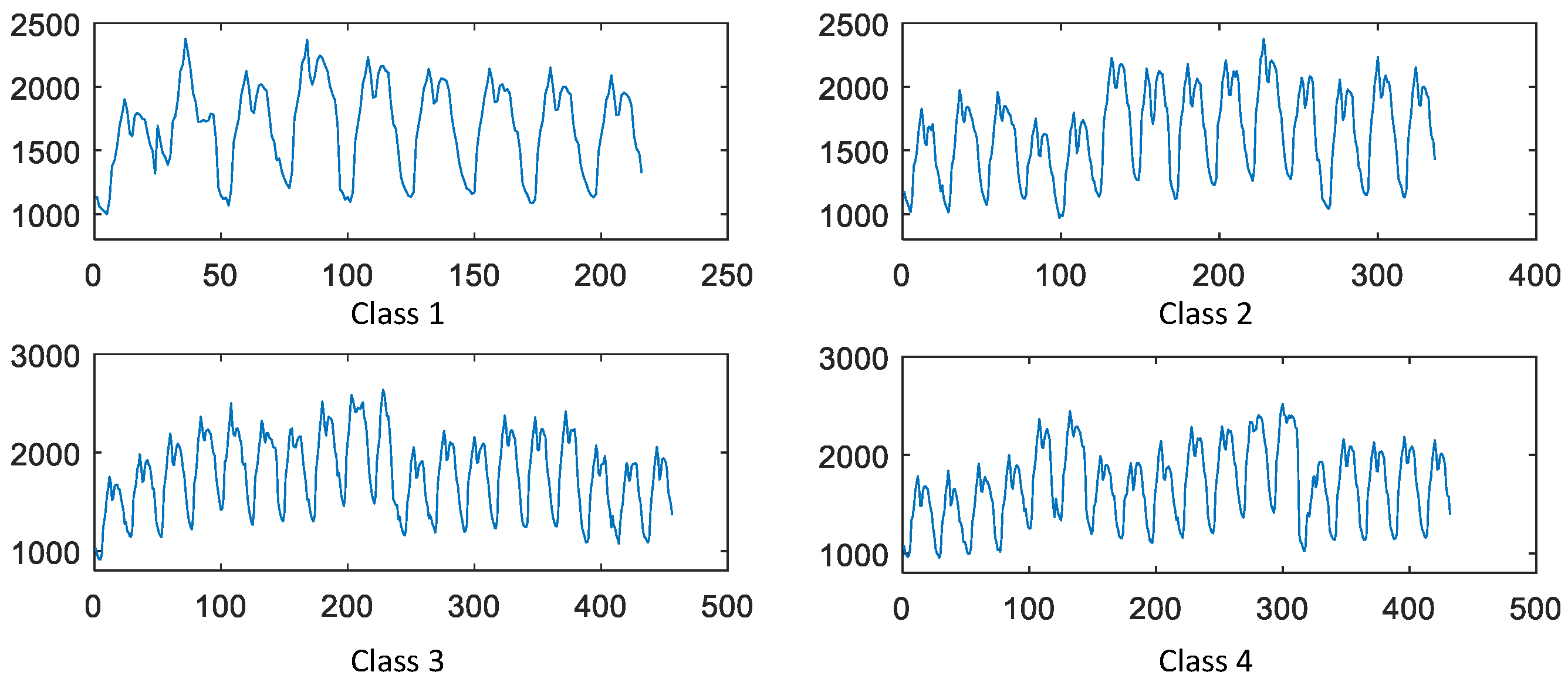
In order to testify the feasibility of the proposed model, the 24-h power load data of Yangquan City are selected for two months. It can be seen that there is nearly no apparent regularity to be obtained from the actual load curves showed in Figure 7 which represents the four classes of load curve. As mentioned above, the three testing days belong to classes 4, 1, 3 respectively and the prediction model is built for the power load forecasting at the same time.

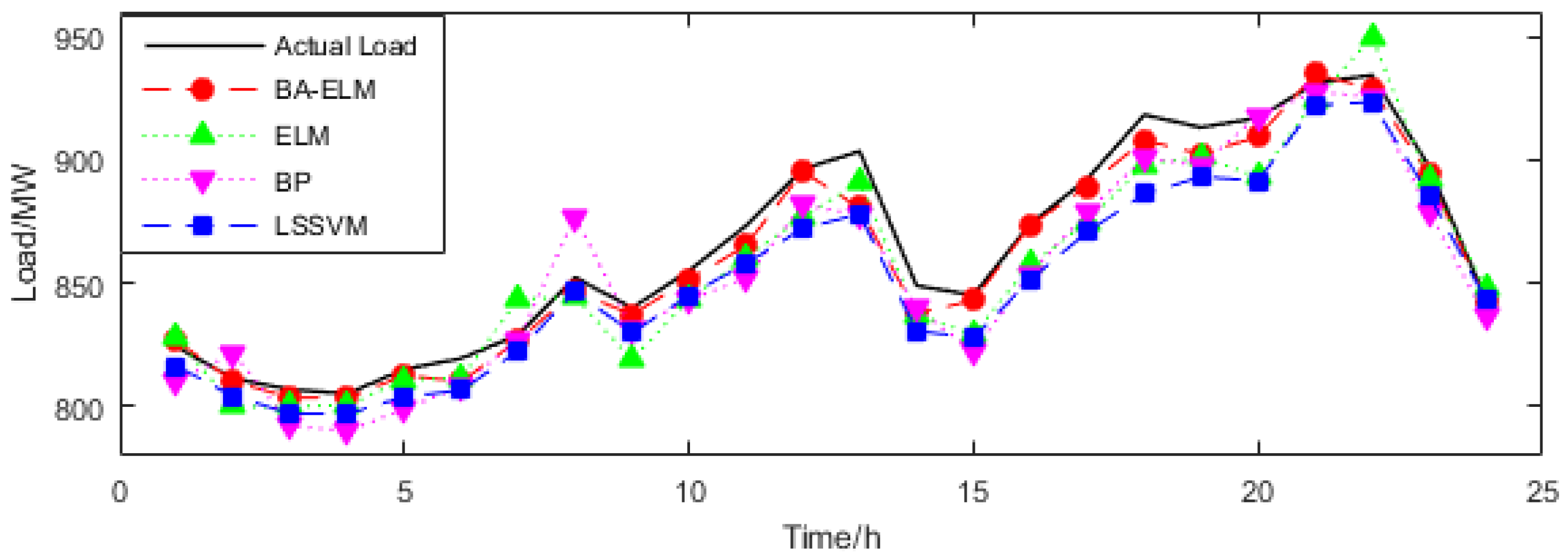
The program runs in MATLAB R2015b under the WIN7 system. The short-term electric load forecasting results of three days of the BA-ELM, ELM, BP and LSSVM models are shown in

Table 7. Actual load and forecasting results on Day 1 (Unit: MV).

Time/h		Actual Data	BA-ELM	ELM	BP	LSSVM
D1	0:00	816.47	819.89	828.77	809.44	813.29
D1	1:00	810.47	808.58	814.55	817.98	801.67
D1	2:00	795.42	805.98	811.75	795.65	794.95
D1	3:00	793.99	797.15	807.93	792.02	795.95
D1	4:00	809.73	806.25	817.20	800.71	801.11
D1	5:00	813.95	812.47	813.37	806.33	805.36
D1	6:00	832.92	826.51	831.65	833.89	820.42
D1	7:00	839.06	855.99	845.01	859.13	847.20
D1	8:00	829.00	831.28	843.41	848.80	830.78
D1	9:00	848.10	852.50	861.05	852.81	842.98
D1	10:00	865.43	870.18	868.09	866.61	856.15
D1	11:00	882.36	893.75	886.89	876.41	873.40
D1	12:00	881.99	895.85	894.77	889.86	878.92
D1	13:00	828.12	839.33	838.77	840.03	831.76
D1	14:00	824.73	844.35	849.89	835.96	831.65
D1	15:00	856.02	871.74	857.20	856.50	854.95
D1	16:00	868.95	900.32	881.47	897.30	872.83
D1	17:00	904.87	900.41	907.67	902.96	889.97
D1	18:00	905.26	911.81	903.64	903.92	894.79
D1	19:00	902.23	909.76	912.14	938.68	897.51
D1	20:00	920.87	939.86	933.37	930.14	926.57
D1	21:00	925.12	931.54	948.12	926.59	923.08
D1	22:00	893.86	891.45	907.02	888.47	883.78
D1	23:00	843.04	844.05	850.39	836.67	841.05

,

Table 8. Actual load and forecasting results on Day 2 (Unit: MV).

Time/h		Actual Data	BA-ELM	ELM	BP	LSSVM
D2	0:00	813.56	823.65	831.48	808.98	817.28
D2	1:00	809.75	813.14	807.71	821.76	805.37
D2	2:00	814.06	805.71	808.58	791.03	798.56
D2	3:00	794.74	802.96	803.47	791.70	799.16
D2	4:00	809.89	807.84	817.35	800.06	805.06
D2	5:00	816.16	815.76	811.90	810.62	808.21
D2	6:00	828.37	827.97	839.11	834.82	823.81
D2	7:00	844.26	855.64	846.80	881.84	849.91
D2	8:00	824.92	831.49	831.84	847.35	832.55
D2	9:00	852.17	853.25	850.02	850.91	846.54
D2	10:00	863.06	870.05	864.05	860.95	859.72
D2	11:00	880.26	896.07	883.27	877.19	875.25
D2	12:00	883.78	891.19	894.20	882.91	880.90
D2	13:00	828.22	840.99	838.46	840.79	833.57
D2	14:00	821.18	846.60	839.96	830.01	831.78
D2	15:00	851.78	875.29	854.88	854.81	855.43
D2	16:00	871.49	897.56	878.00	892.13	874.37
D2	17:00	899.60	908.66	905.04	902.64	890.10
D2	18:00	901.80	910.90	904.57	906.42	897.73
D2	19:00	898.35	920.69	906.55	933.13	896.98
D2	20:00	908.94	938.02	927.70	929.86	926.43
D2	21:00	931.82	929.26	954.66	925.09	926.55
D2	22:00	891.29	892.19	898.24	887.12	887.74
D2	23:00	839.30	843.91	851.50	837.50	845.48

and

Table 9. Actual load and forecasting results on Day 3 (Unit: MV).

Time/h		Actual Data	BA-ELM	ELM	BP	LSSVM
D3	0:00	812.83	826.59	828.03	810.38	816.37
D3	1:00	801.64	810.06	799.93	821.78	804.09
D3	2:00	801.97	803.68	799.95	792.22	797.19
D3	3:00	796.35	803.46	800.56	790.13	797.01
D3	4:00	808.94	812.67	810.88	798.79	803.98
D3	5:00	816.21	810.10	811.44	808.49	806.53
D3	6:00	828.45	826.87	843.63	827.00	822.53
D3	7:00	847.85	846.77	844.31	877.13	846.64
D3	8:00	831.33	837.25	819.12	831.35	829.91
D3	9:00	853.77	851.47	843.37	843.03	845.06
D3	10:00	851.61	865.18	860.53	852.02	857.88
D3	11:00	878.35	895.21	876.79	881.66	872.19
D3	12:00	884.54	880.56	891.03	877.67	877.97
D3	13:00	832.52	837.68	837.29	839.94	830.52
D3	14:00	826.76	842.95	829.22	822.08	828.02
D3	15:00	857.72	873.55	857.38	853.94	851.38
D3	16:00	870.69	889.24	874.85	878.75	870.82
D3	17:00	897.52	907.94	898.13	900.71	886.03
D3	18:00	891.26	902.31	901.23	897.71	893.15
D3	19:00	891.92	909.41	892.96	917.94	891.46
D3	20:00	911.87	934.60	923.71	927.50	921.99
D3	21:00	929.45	928.95	949.86	925.33	923.44
D3	22:00	890.98	893.84	891.63	879.08	885.75
D3	23:00	842.39	842.59	848.01	836.70	843.36

, respectively. For the purpose of explaining the results more clearly, the forecasting values curve of the proposed model and comparisons are shown in Figure 8, Figure 9 and Figure 10. In addition, Figure 11, Figure 12 and Figure 13 reflect the comparisons of relative errors between the proposed model and the others. According to Figure 8, Figure 9 and Figure 10, the deviation can be captured between the actual value and the forecasting results. It can be seen that the forecasting results’ curve of the BA-ELM method are close to the actual data in all testing days, which indicates its higher fitting accuracy.

We commonly consider the RE in the range of [−3%, 3%] and [−1%, 1%] as a standard to testify the performance of the proposed model. Based on these tables and figures, we can determine that: (1) on 28 June, the relative errors of the proposed model and others were all in the range of [−3%, 3%]; only one point (3.52%) of BPNN on 29 June and one point (−3.50%) of LSSVM on 30 June are beyond the range of [−3%, 3%], which indicates that the accuracy is increased after the process of reducing dimensions and clustering. (2) Most relative error points of the BA-ELM locate in the range of [−1%, 1%] on all three days. By contrast, most points of the ELM are beyond the range of [−1%, 1%], which can demonstrate that the BA applied in ELM increases the accuracy and stability of ELM. (3) On 28 June, called Day 1 in this paper, the ELM has 14 predicted points exceed the range of [−1%, 1%], and there is only one point (2.12%) beyond the range of [−2%, 2%] at 21:00; the BP has a dozen predicted points outside the range of [−1%, 1%], and there is one predicted point (−2.05%) beyond the range of [−2%, 2%] at 11:00; the LSSVM has 14 predicted points beyond the range of [−1%, 1%], and there are six predicted points beyond the range of [−2%, 2%], which are −2.38% at 11:00, −2.76% at 12:00, −2.07% at 16:00, −2.85% at 17:00, −2.17% at 18:00 and −2.7% at 19:00. (4) On 29 June, called Day 2 in this paper, the ELM has 10 predicted points exceed the range of [−1%, 1%], and there is only one points beyond the range of [−2%, 2%], which is 2.52% at 21:00; the BP has 16 predicted points exceeding the range of [−1%, 1%], and there are three predicted points beyond the range of [−2%, 2%], which are 3.52% at 7:00, −2.03% at 12:00 and −2.03% at 14:00; the LSSVM has 13 predicted points beyond the range of [−1%, 1%], and there are four predicted points outside the range of [−2%, 2%], which are −2.25% at 12:00, −2.27% at 16:00, −2.77% at 15:00 and −2.17% at 19:00. (5) On 30 June, called Day 3 in this paper, the ELM has 15 predicted points exceed the range of [−1%, 1%], and there are three points beyond the range of [−2%, 2%], which are −2.48% at 8:00, −2.19% at 17:00 and −2.61% at 19:00; the BP has 19 predicted points exceed the range of [−1%, 1%], and there are six predicted points beyond the range of [−2%, 2%], which are 2.91% at 7:00, −2.43% at 10:00, −2.85% at 12:00, −2.73% at 14:00, −2.3% at 15:00 and −2.05% at 22:00; the LSSVM has 18 predicted points beyond the range of [−1%, 1%], and there are nine predicted points outside the range of [−2%, 2%], which are −2.17% at 12:00, −2.03% at 13:00, −2.59% at 14:00, −2.41% at 15:00, −3.5% at 16:00, −2.19% at 17:00 and −2.78% at 18:00. From the global view of relative errors, the forecasting accuracy of BA-ELM is better than the other models, since it has the most predicted points in the ranges [−1%, 1%], [−2%, 2%] and [−3%, 3%]. Compared with BPNN and LSSVM, the relative errors of ELM are low. The reason is that the BPNN can have advantages when dealing with the big sample, but its forecasting results are not very good when dealing with a small sample problem like short-term load forecasting. The kernel parameter and penalty factor setting manually of LSSVM are difficult to confirm, which has a significant influence on the forecasting accuracy.

The number of points that are less than 1%, 2%, 3% and more than 3% and the corresponding percentage of them in the predicted points are accounted for, respectively. The statistical results are shown in

Table 10. Accuracy estimation of the prediction point for the test set.

Prediction Model	<1%		>1% and <2%		>2% and <3%		>3%
	Number	Percentage	Number	Percentage	Number	Percentage	Number	Percentage
BA-ELM	61	84.72%	10	13.89%	1	1.39%	0	0
ELM	33	45.83%	33	45.83%	6	8.34%	0	0
BPNN	24	33.33%	37	51.39%	10	14.29%	1	1.39%
LSSVM	27	37.50%	26	36.11%	18	25%	1	1.39%

. It can be seen that there are 61 predicted points whose the AE of the BA-ELM model is less than 1%, which accounts for 84.72% of the total amount; and 10 predicted points in the range of [1%, 2%], accounting for 13.89% of the total amount; and only 1 predicted point in the range of [2%, 3%], accounting for 1.39% of the total amount. Moreover, there are no predicted points whose AE is more than 3%, accounting for 0% of the total amount. It can be concluded that the forecasting performance of the proposed model is superior, and its accuracy is higher, which means the BA-ELM model is suitable for short-term load forecasting.

The average RMSE and MAPE of the BA-ELM, ELM, BPNN and LSSVM models are listed in

Table 11. Average forecasting results of four models.

	Model	BA-ELM	ELM	BPNN	LSSVM
Index
RMSE (MW)		5.89	11.08	12.74	14.47
MAPE (%)		0.49	1.13	1.29	1.43
MAE (MW)		4.27	9.81	11.14	12.51

. In order to show the comparisons clearly, the RMSE, MAE and MAPE of four forecasting models in three testing days are show in Figure 14, Figure 15 and Figure 16. It can be concluded that both of the RMSE, MAE and MAPE of BA-ELM are lower on three testing days. On 28 June, the RMSE, MAE and MAPE of ELM are slightly bigger than BP, but smaller than that of LSSVM. On 29 June, the RMSE, MAE and MAPE of ELM are smaller than that of BP and LSSVM. The RMSE, MAE and MAPE of BP are close to that of LSSVM. On 30 June, the RMSE, MAE and MAPE of ELM are smaller than BP and LSSVM’s, and that of BP are smaller than LSSVM’s. To sum up, combining this with the Table 11, the average behavior of four models are BA-ELM, ELM, BPNN and LSSVM from low to high successively.

5. Conclusions

With the development of society and technology, research to improve the precision of load forecasting has become necessary because short-term power load forecasting can be regarded as a vital component of smart grids that can not only reduce electric power costs but also ensure the continuous flow of electricity supply. This paper selected 22 original indexes as the influential factors of power load and factor analysis was employed to discuss their correlation and economic connotations, from which it can be seen that the historical data occupied the largest contribution rate and the meteorological factor followed thereafter. Consequently, the paper introduced the auto correlation and partial auto correlation function to further explore the relationship between historical load and current load. Considering the influence of similar day, ant colony clustering was adopted to cluster the sample for the sake of searching the days with analogous features. Finally, the extreme learning machine optimized by a bat algorithm was conducted to predict the days that are chosen to test. The simulation experiment carried out in Yangquan City in China verified the effectiveness and applicability of the proposed model, and a comparison with benchmark models illustrated the superiority of the novel hybrid model successfully.

References

- Hernandez, L.; Baladron, C.; Aguiar, J.M.; Carro, B.; Sanchez-Esguevillas, A.J.; Lloret, J.; Massana, J. A Survey on Electric Power Demand Forecasting: Future Trends in Smart Grids, Microgrids and Smart Buildings. IEEE Commun. Surv. Tutor. 2014, 16, 1460–1495. [Google Scholar] [CrossRef]
- Lv, Z.J. Application of regression analysis in power load forecasting. Hebei Electr. Power 1987, 1, 17–23. [Google Scholar]
- Li, P.O.; Li, M.; Liu, D.C. Power load forecasting based on improved regression. Power Syst. Technol. 2006, 30, 99–104. [Google Scholar]
- Li, X.; Zhang, L.; Yao, S.; Huang, R.; Liu, S.; Lv, Q.; Zhang, L. A New Algorithm for Power Load Forecasting Based on Time Series. Power Syst. Technol. 2006, 31, 595–599. [Google Scholar]
- Metaxiotis, K.; Kagiannas, A. Artificial intelligence in short term electric load forecasting: A state-of-the-art survey for the researcher. Energy Convers. Manag. 2003, 44, 1525–1534. [Google Scholar] [CrossRef]
- Hippert, H.S.; Pedreira, C.E.; Souza, R.C. Neural Networks for Short-Term Load Forecasting: A Review and Evaluation. IEEE Trans. Power Syst. 2001, 16, 44–55. [Google Scholar] [CrossRef]
- Park, D.C.; El-Sharkawi, M.A.; Marks, R.J.; Atlas, L.E.; Damborg, M.J. Electric Load Forecasting Using an Artificial Network. IEEE Trans. Power Syst. 1991, 6, 422–449. [Google Scholar] [CrossRef]
- Hernandez, L.; Baladrón, C.; Aguiar, J.M.; Carro, B.; Sanchez-Esguevillas, A.J.; Lloret, J. Short-Term Load Forecasting for Microgrids Based on Artificial Neural Networks. Energies 2013, 6, 1385–1408. [Google Scholar] [CrossRef]
- Yu, F.; Xu, X. A short-term load forecasting model of natural gas based on optimized genetic algorithm and improved BP neural network. Appl. Energy 2014, 134, 102–113. [Google Scholar] [CrossRef]
- Hu, R.; Wen, S.; Zeng, Z.; Huang, T. A short-term power load forecasting model based on the generalized regression neural network with decreasing step fruit fly optimization algorithm. Neurocomputing 2017, 221, 24–31. [Google Scholar] [CrossRef]
- Li, Y.C.; Fang, T.J.; Yu, E.K. Study on short—Term load forecasting using support vector machine. Proc. CSEE 2003, 23, 55–59. [Google Scholar]
- Zhao, D.F.; Wang, M. Short—Term load forecasting based on support vector machine. Proc. CSEE 2002, 22, 26–30. [Google Scholar]
- Mesbah, M.; Soroush, E.; Azari, V.; Lee, M.; Bahadori, A.; Habibnia, S. Vapor liquid equilibrium prediction of carbon dioxide and hydrocarbon systems using LSSVM algorithm. J. Supercrit. Fluids 2015, 97, 256–267. [Google Scholar] [CrossRef]
- Huang, G.B.; Zhu, Q.Y.; Siew, C.K. Extreme learning machine: Theory and applications. Neurocomputing 2006, 70, 489–501. [Google Scholar] [CrossRef]
- Huang, G.B.; Zhou, H.; Ding, X.; Zhang, R. Extreme learning machine for regression and multiclass classification. IEEE Trans. Syst. Man Cybern. Part B 2012, 42, 513–529. [Google Scholar] [CrossRef] [PubMed]
- Yang, X.S.; Hossein Gandomi, A. Bat algorithm: A novel approach for global engineering optimization. Eng. Comput. 2012, 29, 267–289. [Google Scholar] [CrossRef]
- Zhang, J.W.; Wang, G.G. Image Matching Using a Bat Algorithm with Mutation. Appl. Mech. Mater. 2012, 203, 88–93. [Google Scholar] [CrossRef]
- Mishra, S.; Shaw, K.; Mishra, D. A New Meta-heuristic Bat Inspired Classification Approach for Microarray Data. Procedia Technol. 2012, 4, 802–806. [Google Scholar] [CrossRef]
- Nakamura, R.Y.; Pereira, L.A.; Costa, K.A.; Rodrigues, D.; Papa, J.P.; Yang, X.S. BBA: A Binary Bat Algorithm for Feature Selection. In Proceedings of the 25th SIBGRAPI Conference on Graphics, Patterns and Images, Ouro Preto, Brazil, 22–25 August 2012; pp. 291–297. [Google Scholar]
- Niu, D.; Dai, S. A Short-Term Load Forecasting Model with a Modified Particle Swarm Optimization Algorithm and Least Squares Support Vector Machine Based on the Denoising Method of Empirical Mode Decomposition and Grey Relational Analysis. Energies 2017, 10, 408. [Google Scholar] [CrossRef]
- Liang, Y.; Niu, D.; Ye, M.; Hong, W.C. Short-Term Load Forecasting Based on Wavelet Transform and Least Squares Support Vector Machine Optimized by Improved Cuckoo Search. Energies 2016, 9, 827. [Google Scholar] [CrossRef]
- Sun, W.; Liang, Y. Least-Squares Support Vector Machine Based on Improved Imperialist Competitive Algorithm in a Short-Term Load Forecasting Model. J. Energy Eng. 2014, 141, 04014037. [Google Scholar] [CrossRef]
- Hooshmand, R.A.; Amooshahi, H.; Parastegari, M. A hybrid intelligent algorithm based short-term load forecasting approach. Int. J. Electr. Power Energy Syst. 2013, 45, 313–324. [Google Scholar] [CrossRef]
- Bahrami, S.; Hooshmand, R.A.; Parastegari, M. Short term electric load forecasting by wavelet transform and grey model improved by PSO (particle swarm optimization) algorithm. Energy 2014, 72, 434–442. [Google Scholar] [CrossRef]
- Yeom, C.U.; Kwak, K.C. Short-Term Electricity-Load Forecasting Using a TSK-Based Extreme Learning Machine with Knowledge Representation. Energies 2017, 10, 1613. [Google Scholar] [CrossRef]
- Yang, X.S. A New Metaheuristic Bat-Inspired Algorithm. Comput. Knowl. Technol. 2010, 284, 65–74. [Google Scholar]
- Deng, W.Y.; Zheng, Q.H.; Chen, L.; Xu, X.B. Study on fast learning method of neural network. Chin. J. Comput. 2010, 33, 279–287. [Google Scholar] [CrossRef]
Figure 1.
The framework of the extreme learning machine.
Figure 2.
The flowchart of the ant colony clustering algorithm.
Figure 3.
The flowchart of the factor analysis-ant colony clustering-bat algorithm-extreme learning machine (FA-ACC-BA-ELM) model.
Figure 4.
The partial auto correlation result of the overall power load.
Figure 5.
The partial auto correlation result of the load with the same interval.
Figure 6.
The iterations process of the bat algorithm (BA).
Figure 7.
The four types of power load curve.
Figure 8.
Compared load forecasting results on 28 June.
Figure 9.
Compared load forecasting results on 29 June.
Figure 10.
Compared load forecasting results on 30 June.
Figure 11.
Compared relative errors of four models on 28 June.
Figure 12.
Compared relative errors of four models on 29 June.
Figure 13.
Compared relative errors of four models on 30 June.
Figure 14.
Root-mean-square error (RMSE) of different models in testing period.
Figure 15.
Mean absolute percentage error (MAPE) of different models in testing period.
Figure 16.
Mean absolute error (MAE) of different models in testing period.