Short-Term Load Forecasting for Electric Bus Charging Stations Based on Fuzzy Clustering and Least Squares Support Vector Machine Optimized by Wolf Pack Algorithm

Department of Economic Management, North China Electric Power University, Baoding 071003, China, [email protected]
Energies 2018, 11(6), 1449; https://doi.org/10.3390/en11061449
Submission received: 22 May 2018
/
Revised: 31 May 2018
/
Accepted: 1 June 2018
/
Published: 4 June 2018
(This article belongs to the Special Issue Short-Term Load Forecasting by Artificial Intelligent Technologies)
Abstract
:Accurate short-term load forecasting is of momentous significance to ensure safe and economic operation of quick-change electric bus (e-bus) charging stations. In order to improve the accuracy and stability of load prediction, this paper proposes a hybrid model that combines fuzzy clustering (FC), least squares support vector machine (LSSVM), and wolf pack algorithm (WPA). On the basis of load characteristics analysis for e-bus charging stations, FC is adopted to extract samples on similar days, which can not only avoid the blindness of selecting similar days by experience, but can also overcome the adverse effects of unconventional load data caused by a sudden change of factors on training. Then, WPA with good global convergence and computational robustness is employed to optimize the parameters of LSSVM. Thus, a novel hybrid load forecasting model for quick-change e-bus charging stations is built, namely FC-WPA-LSSVM. To verify the developed model, two case studies are used for model construction and testing. The simulation test results prove that the proposed model can obtain high prediction accuracy and ideal stability.
1. Introduction
In recent years, low-carbon cities have become a common pursuit around the world, which is faced with increasing energy crises and environmental problems [1]. Electric buses (e-buses) have developed quickly with the burgeoning construction of low-carbon cities [2]. As important supporting facilities, charging stations bring new challenges to optimal dispatching and safe operation of the power grid due to great volatility, randomness and intermittence of the load [3]. Therefore, it is of great significance to conduct research on load characteristics analysis and short-term load forecasting. On one hand, this contributes to the optimal combination of generator units in terms of power system, economical dispatch, optimal power flow and electricity market transactions. On the other hand, it provides a decision basis for construction planning, energy management, orderly charging and economical operation for charging stations, which can guarantee and promote the development of low-carbon cities. Therefore, research on short-term load forecasting for quick-change e-bus charging stations has been conducted to provide data support and a theoretical basis for the large-scale construction of charging stations.
Nowadays, scholars have conducted a large amount of research on load forecasting for charging stations. The prediction methods are primarily divided into two categories: traditional forecasting approaches, such as time series [4], regression analysis [5], and fuzzy prediction [6], and artificially intelligent algorithms. Conventional prediction methods aiming at load forecasting for e-bus charging stations are mainly established on the foundation of probability and statistics theory. Ashtari et al. [7] installed GPS equipment on 76 representative plug-in electric vehicles in Winnipeg, Canada, and collected driving data for the whole year. The load forecasting was conducted in consideration of the actual charging sate of battery, stopping time, parking type and vehicle power system. In [8], four variables, including the number of vehicles needing battery change per hour, the starting time of charging, driving distance and charging duration, were taken into account under an uncontrolled swapping and charging scenario. On this basis, the Monte Carlo method integrated non-parameter estimation approach was employed in load forecasting for electric vehicle charging stations. As we can see, traditional prediction methods have the advantages of mature theory, perfect verification approaches and simple calculation, but the weaknesses of a single applicable object and unideal prediction precision are also notable. Accordingly, it is of great importance to apply intelligent forecasting techniques to load forecasting of charging stations with the rapid development of artificial intelligence technology.
Intelligent algorithms for load forecasting chiefly consist of artificial neural networks (ANNs) and support vector machine (SVM) [9]. Back propagation neural network (BPNN), treated as representative of ANNs, is suitable for load prediction of quick-change e-bus charging stations. For example, [10] analyzed the load characteristics and influential factors, as well as executing a BPNN model to predict the short-term load based on the measured data of quick-change e-bus charging stations at the Beijing Olympic Games. The approach in this study proved to be useful. Additionally, some scholars have adopted ANNs for short-term load forecasting of other power systems. Xiao et al [11] combined single spectrum analysis (SSA) with modified wavelet neural network (WNN) to establish a reliable short-term forecasting approach in the field of load, wind speed and electricity price. Reference [12] proposed a novel ensemble prediction method for short-term load forecasting on the foundation of the extreme learning machine (ELM), where four improvements were made to the ELM. The results showed that the prediction accuracy of the proposed technique was superior to the standard ANNs. However, the drawbacks of ANNs include slow convergence and easy trapping into the local minimum, which greatly limit the forecasting precision and stability. SVM model can effectively address these problems [13]; thus, this approach has been widely used in the research of load forecasting. Reference [14] designed an incremental learning model on the basis of SVM to implement load prediction under batch arrival with a large sample. In reference [15], an SVM model based on the selection of similar days for daily load forecasting of electric vehicles was come up with. Correlation analysis was presented to extract the influential factors and grey correlation theory was utilized to obtain a small sample set of similar days. Compared with ANNs, the SVM model achieved better results for load forecasting. Nevertheless, the transformation of the kernel function to convert the problem into quadratic programming reduces the efficiency and accuracy of traditional SVM [16].
Least squares support vector machine (LSSVM) is a modified form for SVM where the least squares linear system serves as the loss function to avoid quadratic programming, and the kernel function is employed to transform prediction problems into equations, as well as to convert inequality constraints into equality ones, which can improve the forecasting accuracy and speed [17]. Reference [18] introduced LSSVM to predict the annual load in China with the rolling mechanism. The good results verified the applicability of LSSVM in load forecasting. Reference [19] built a hybrid model integrated LSSVM with cuckoo search algorithm (CS) for short-term load forecasting. The findings indicated that this proposed technique could obtain good prediction results. Remarkably, LSSVM has not yet been applied to load forecasting for quick-change e-bus charging station. The learning and generalization ability of LSSVM model hinges on the selection of two parameters, namely, regularization parameter and kernel parameter . As a result, it is necessary to utilize an appropriate intelligent algorithm to determine these values. The commonly employed optimization methods include genetic algorithm (GA) [20], particle swarm optimization (PSO) [21], CS [22] and bat algorithm (BA) [23]. However, GA has the disadvantages of premature convergence, complex computation, small processing scale, poor stability and difficulty in coping with nonlinear constraints. The poor accuracy of local search of PSO cannot fully satisfy the need of parameter optimization in LSSVM. The shortcoming of CS and BA is that they easily fall into local optimums, leading to reduction in prediction accuracy. Wolf pack algorithm (WPA), as a new metaheuristic approach, is introduced in this paper to optimize the parameters in LSSVM. This technique possesses good global convergence and computational robustness due to insensitivity of the change of parameters in WPA [24].
As a result of the complexity and diversity of the influential factors for load forecasting in quick-change e-bus charging stations, it is of great necessity to select proper inputs for the prediction, so that redundant data can be reduced and computing efficiency can be improved [25]. Fuzzy clustering (FC) is a mathematical technique that classifies objects according to their characteristics [26]. In view of the fact that the daily load curves with similar influential factors of charging stations are basically consistent, good prediction results can be achieved by the use of samples on similar days. Consequently, a transitive closure algorithm grounded on a fuzzy equivalent matrix in FC is selected in this paper, which can extract samples similar to the predicted day. It can not only avoid the blindness of choosing similar days by experience, but also overcome the adverse effects of unconventional load data caused by sudden change of factors on LSSVM training.
Therefore, the influential factors for the load in quick-change e-bus charging stations are analyzed in this paper, and a load forecasting model combining FC with LSSVM and optimized by WPA (FC-WPA-LSSVM) is established here. The rest of paper is organized as follows: Section 2 conducts an analysis of the daily load characteristics for quick-change e-bus charging stations based on related statistical data and studies various influential factors including day types, meteorological conditions and bus dispatch; Section 3 provides a brief description of FC, LSSVM and WPA, as well as the complete prediction framework; Section 4 introduces an experimental study to validate the proposed method; and Section 5 makes further validation. In Section 6, conclusions are obtained.
2. Analysis of Load Characteristics of E-Bus Charging Stations
The load of a large quick-change e-bus charging station in Baoding, China, is provided in this paper. When the bus comes into the station, the battery with electricity depletion is changed by the quick-change robot, which is further connected to the charging platform. Then, a battery filled with electricity is installed in the bus. After that, the e-bus goes into a specific area to wait for dispatch instructions. According to the dispatch, the e-bus appears at the charging station after 8:00 a.m. each day, which leads to a rise in load. The chargers will not stop working until the battery charging of the last e-bus is completed. At that time, the load decreases to the lowest point.
A typical daily load curve of the e-bus charging station is shown in Figure 1, which displays the active power per hour in a day. In common with the traditional load curve, there exist obvious crests and troughs. However, the curve of the e-bus charging station fluctuates greatly, and apparent distinctions appear among different curves, whereby the load in winter and summer is high, while the load in spring and autumn is low. All of these characteristics create difficulties for the daily load forecasting of the charging station.
The load is influenced by various factors. Here, three variables, including day types, meteorological conditions and e-bus dispatching, are selected. Unlike traditional motor vehicles, the source of power for electric buses is all electric power. When there is a traffic jam, there is no energy loss for electric buses. Therefore, traffic congestion factors do not affect the load of charging stations.
2.1. Day Types
E-bus charging stations serve the electricity supply of urban e-buses. In accordance with the habits and demands of citizens, the scheduling of e-buses between weekdays and weekends is different across the week, which also results in obvious differences in the load curve.
Table 1 displays the annual mean of daily maximum load and daily average load for the e-bus charging station in Baoding in 2016 on the basis of day types. It can be seen that the loads on workdays are relatively higher than those on weekends. Thus, a week can be divided into two categories, namely workdays, including Monday to Friday, and weekends, which contain Saturday and Sunday. Special holidays, such as Dragon Boat Day, Labor Day or National Day, can be separated as a new type alone.
2.2. Meteorological Conditions
Data related to meteorological conditions and the power load of Baoding from August 16 to September 15, 2017 (31 days in total) are collected and shown in Figure 2. The meteorological conditions include the daily maximum temperature, daily weather, daily average wind speed and daily average humidity. In the daily weather condition, “1” is used to represent a sunny day, “2” is used to represent cloudy day, and “3” is used to represent a rainy or snowy day. As can be seen in Figure 2, there is a significant positive correlation between daily maximum temperature and power load, and weather and power load show a negative correlation. However, there is no obvious relationship between the average wind speed factor and load, and the average humidity factor is similar. Thus, it can be found that the load of e-bus charging stations is remarkably affected by temperature, as well as by rainy and snowy days, while the influence of other meteorological conditions such as humidity and wind speed is so weak that they can be omitted. Therefore, temperature and rainy and snowy days are selected as influential indicators in this paper.
Similar to traditional power loads, the daily load of the charging station increases owing to the use of air conditioners on e-buses when the temperature change of coldness and warmth is aggravated. Since temperature has an important influence on battery capacity, as well as on the charging and discharging process, the charging time is diverse at different temperatures, which also leads to distinct trends of load. The daily load curves from September 12 to 14, 2017 are taken as an example, in which the total number of charged e-buses in these three days was about 60 and the maximum temperature dropped from 35 to 24. As seen in Figure 3, the violent fluctuation of air temperature in adjacent days causes great changes in daily load curves. Thus, it is necessary to take temperature as an influential factor in the selection of subsequent similar day samples.
Taking the daily load curves on August 29 and August 30 in 2017 as an example, weather conditions can be divided into sunny days and rainy days. Figure 4 illustrates the relationship between weather conditions and the daily load of the charging station. It proves that daily maximum load decreases on rainy and snowy days on account of the deceleration of e-buses, which leads to a decrease in the daily driving mileage and charging times as well as the reduction of total load in the charging station. To this end, rainy and snowy days are another vital factor that affects the load characteristics of e-bus charging stations.
2.3. Bus Dispatching
The scheduling of departure time and off-running time is a momentous task for bus operation companies. In light of the daily plan of bus dispatching, different charging intensities of e-buses in the station cause changes in the daily load curve in the charging station at different periods. Moreover, diverse demands of the public, traffic jams, and sudden situations require the addition of temporary e-buses to enhance transport capacity, which brings about changes in bus scheduling on different days. Bus dispatching is one of the direct reasons for the fluctuation of daily load curve and the distinction of load curves among days. According to the dispatch plan made in advance, the total number of e-buses that need to be charged on a predicted day can be estimated; namely, the accumulated number of e-buses charged daily, which is used as an indicator to reflect the effect of bus dispatching on the load of the quick-change e-bus charging station.
3. Methodology
3.1. Fuzzy Clustering
FC analysis is a mathematical technique that achieves classification of objects through the establishment of fuzzy similarity relations based on their characteristics, familiarity and comparability. The fuzzy equivalent matrix dynamic clustering method is implemented in this paper.
Suppose samples on the predicted day, that is . Each sample comprises indicators, expressed as , .
The specific steps of FC can be explained as follows:
(1) Data standardization. Considering different dimensions and orders of magnitude, the data must be standardized as Equation (1) [27].
where is the raw data, and are the minimum and maximum of , respectively, is the standardized data.
(2) Establishment of fuzzy similarity relation matrix. In order to measure the comparability of the classified samples, a fuzzy similarity relation matrix needs to be constructed by similarity of coefficient approach, distance or closeness. An absolute value index method is introduced here [28], as expressed in Equation (2).
Then the transitive closure of can be obtained by square synthesis.
(3) Dynamic clustering. Select an appropriate threshold to separate . The clustering results are up to the level of . When drops from 1 to 0, a dynamic clustering graph is obtained by changing the rough classification to a fine one. The best value of can be acquired based on its change rate [29].
where is the clustering order of in a descending form; and are the number of elements in and clusters, respectively; and are the confidence levels in and clusters, respectively. If , is treated as the best threshold. Thus, samples can be separated into several categories and each type contains a different number of samples.
(4) Classification recognition. The category consistent with the forecasted day needs to be identified after sample classification. The Euclidean distance is calculated between the predicted day and the above categories one by one [26]:
where is the characteristic vector on the predicted day, represents the characteristic vector of each category. This paper takes the type with the shortest Euclidean distance as the classification of the forecasted day to make the prediction.
3.2. Least Squares Support Vector Machine
As an extension of SVM, LSSVM transforms the inequality constraints into equality ones and converts quadratic programming problems into linear equation ones, which is conducive to the improvement of convergence speed [30].
Set the training samples as , where is the total number of samples. The regression model can be expressed as follows [31]:
where is a function that maps the training samples into a highly dimensional space, and represent the weight and bias, respectively.
For LSSVM, the optimization problem can be defined as Equation (6) [32]:
where is the regularization parameter that balances the complexity and precision of the model. equals the error.
To obtain the solution, the Lagrange function can be established as Equation (8).
where is the Lagrange multipliers. Take the derivatives of each variable in the function and make them equal zero:
Eliminate as well as and transform it into the following problem:
where
The solution can be obtained based on the linear equations above:
where is the kernel function that meets Mercer’s condition. The radial basis function (RBF) is employed as the kernel function here on the basis of its wide convergence region and extensive application scope, as shown in Equation (16).
where represents the kernel parameter that reflects the characteristic of training samples and has influence on generalization ability of the technique.
As we can see, the performance improvement of LSSVM model is greatly dependent on the appropriate setting of the following parameters: regularization parameter and kernel parameter [33].
3.3. Wolf Pack Algorithm
In consideration of the blindness of manual selection in LSSVM model parameters, the optimal value of regularization parameter and kernel parameter of LSSVM is obtained through the wolf pack algorithm. The WPA technique is inspired by research on the hunting behaviors of wolves [34]. According to their roles in hunting, wolves can be divided into three types: head wolves, safari wolves and feral wolves, who work together to complete the task. Random walk, call to action and siege are three main behaviors of wolves, which are simulated in the WPA model. The determination of the head wolf and the replacement of the wolf pack follow the common rules that the “winner is the king” and “the survival of the fittest”, respectively [35]. WPA is illustrated in Figure 5.
The principle and steps of WPA are summarized as follows [36]:
(1) Initialize wolf pack. Suppose in dimensional space, there are wolves, wherein the location of the -th wolf is set as:
The initial position is generated as Equation (18):
where represents random numbers within the range [0,1], and and are the upper limit and lower limit of the search space, respectively.
(2) Generate the head wolf. The wolf at with the best target function is selected as the head one. The head wolf does not update its position in the hunting process or participate in hunting; instead, it is directly iterated. If , , where represents the location of the safari wolf . Otherwise, the safari wolf randomly walks in directions until the maximum value is achieved or the location cannot be further optimized; then the search is stopped. is the location at -th point in -th dimension of the -th wolf.
(3) Keep close to the prey. The head wolf pushes the wolf pack to update their positions through call to action. The new position of the -th wolf in -dimension is described as Equation (20):
where is the step length of wolves in search, represents the step length of wolves towards the target, and are the location of the -th wolf and the corresponding head wolf in -dimension, respectively.
(4) Encircle the prey. The head wolf sends signals to the surrounding wolf pack after finding the prey so that the encirclement and suppression of the target prey can be completed, as shown in Equations (21) and (22):
where equals the number of iterations, is the step length at the time of encirclement and suppression, is the location of the head wolf that sends the signal, and is the location of the -th wolf in the -th iteration.
(5) The mechanism of competition and regeneration of the wolf pack. In encirclement and suppression, the wolves that fail to get food will be eliminated and the rest of wolves will be retained. Simultaneously, new wolves are randomly generated in the same number as the eliminated ones.
(6) Judge whether the maximum number of iterations has been reached. If the maximum number of iterations has been reached, the position of the wolf is output; that is, the optimal value of the LSSVM’s parameters. If the maximum number of iterations has not been reached, then return to step 2.
3.4. Establishment of the Hybrid Forecasting Model
This paper firstly analyzes the influential load factors for quick-change e-bus charging stations, and FC is implemented to extract similar days to the predicted one as the training samples. Then, WPA is integrated with the LSSVM model to obtain the optimal values of and . Finally, an analysis is performed on the forecasting results. The framework of the proposed hybrid approach is displayed in Figure 6.
4. Case Study
Base on the daily load, meteorological data and operation information of an e-bus charging station in Baoding, China, in 2017, a case study was carried out for the purpose of demonstrating the efficiency of the proposed model in load forecasting for e-bus charging station. The load data was provided by State Grid Hebei Electric Power Company in China, and the input data was provided by the local meteorological department. This paper adopts Matlab R2014b (Gamax Laboratory Solutions Kft., Budapest, Hungary) to program, and as for the test platform environment, an Intel Core i5-6300U (Intel Corporation, Santa Clara, CA, USA), 4G memory and Windows 10 Professional (Microsoft corporation, Redmond, WA, USA) Edition system was used. In order to eliminate the particularity of the target days and examine the generalization performance of the established technique, the data for one day from each of the four seasons was selected as test samples; that is, April 15, July 15, October 15 and January 15 were chosen as test samples for spring, summer, autumn and winter, respectively.
4.1. Input Selection and Pre-Processing
Based on the analysis of load characteristics in the e-bus charging station in Section 2, a set of eight variables was used as the input, including day type, maximum temperature, minimum temperature, weather condition, the accumulated daily number of charged e-buses and the loads at the same moment in the previous three days. Days can be divided into three categories: workdays (Monday to Friday), weekends (Saturday and Sunday) and legal holidays were valued at 1, 0.5 and 0, respectively. Weather conditions were separated into two types, where sunny and cloudy days were valued at 1, and rainy and snowy days were valued at 0.5. The loads at the same moment in the previous three days refer to those nearest the predicted day in similar samples after clustering according to the rule that “Everything looks small in the distance and is big on the contrary.” The temperature, load data, and daily accumulated charged e-buses should be normalized as presented in Equation (1).
4.2. Model Performance Evaluation
It’s important to effectively evaluate the load forecasting results for e-bus charging stations, and the performance of the prediction models is usually assessed by statistical criteria: the relative error (RE), root mean square error (RMSE), mean absolute percentage error (MAPE) and average absolute error (AAE). The smaller the values of these four indicators are, the better the forecasting performance is. In addition, the indicators named RMSE, MAPE and AAE can reflect the overall error of the prediction model and the degree of error dispersion. The smaller the values of these three indicators are, the more concentrated the distribution of errors is. The four generally adopted error criteria are displayed as follows:
(1) Relative error (RE)
(2) Root mean square error (RMSE)
(3) Mean absolute percentage error (MAPE)
(4) Average absolute error (AAE)
where and are the actual load and the forecasted one of charging station, respectively; equals the number of groups in the dataset. The smaller these evaluation indicators are, the higher the prediction accuracy is.
4.3. Results Analysis
The parameters of the proposed model are set as: the total wolf pack , iteration number , , , , . The forecasting results are shown in Figure 7.
As can be seen from Figure 7, the proposed model is very close to the actual load curve in each season and has a good degree of fit. Figure 8 shows the relative error of the prediction results. It can be seen that the relative error of the prediction results of the FC-WPA-LSSVM model is controlled within the range [−3%, 3%], and the degree of deviation is acceptable.
4.4. Discussion
In order to verify the performance of the forecasting approach, three basic techniques, including WPA-LSSVM [37], LSSVM [38], and BPNN [39], were introduced to make a comparison. The parameter settings in WPA-LSSVM were consistent with those in the established model. In LSSVM, the regularization parameter and the kernel parameter were valued at 12.6915 and 12.0136, respectively. In BPNN, tansig was utilized as the transfer function in the hidden layer, and purelin was employed as the transfer function in the output layer. The maximum number of convergence was 200, the error was equal to 0.0001, and the learning rate was set as 0.1. The determination of the initial weights and thresholds depend on their own training. Figure 9 illustrates the load forecasting results of FC-WPA-LSSVM, WPA-LSSVM, LSSVM and BPNN. Figure 10 presents the values of RE for each prediction method.
From Figure 9 and Figure 10, it can be seen that the prediction error range of FC-WPA-LSSVM was controlled to within [−3% + 3%], where the minimum error (7:00 in the spring test) and the maximum error (18:00 in the autumn test) were 0.08% and −2.98%, respectively. Among them, 10 error points of the results were within [−1%, 1%], namely 7:00, 11:00 and 16:00 in the spring test, 1:00, 2:00, 9:00, 16:00, 23:00 in the summer test, 6:00 in the autumn test, 19:00 in the winter test; the corresponding values of RE were 0.08%, −0.49%, −0.52%, −0.71%, −0.98%, −0.74%, −0.85%, 0.71%, −0.81% and 0.31%, respectively. In addition, 19 error points of WPA-LSSVM were controlled to within [−3%, 3%], while the corresponding number for LSSVM was 17, of which 2 points of WPA-LSSVM were within the range [−1%, 1%], namely at 10:00 in the spring test (RE = −0.86%) and 9:00 in the winter test (RE = − 0.79%), but all error points of LSSVM were outside the range [−1%, 1%]. The minimum errors of WPA-LSSVM and LSSVM were −0.79% and −1.07% respectively, while their maximum errors were 6.6% and −7.59%, respectively. The errors of the BPNN model were mostly within the ranges [−6%, −4%] or [4%, 6%], where the maximum and minimum of RE were individually equal to 1.36% and 8.73%, respectively. In this regard, the forecasting accuracy ranked from the highest to the lowest was: FC-WPA-LSSVM, WPA-LSSVM, LSSVM, and BPNN. Hence, FC can effectively avoid the blindness in the selection of similar days through experience. In contrast with LSSVM, administering WPA improves the prediction precision by virtue of the parameter optimization of LSSVM. It is without doubt that the forecasting accuracy of some points in FC-WPA-LSSVM is worse than the other three approaches; for instance, the error of FC-WPA-LSSVM was 1.76% at 22:00 in the spring test, which was greater than WPA-LSSVM and BPNN.
The performance comparison results of the forecasting models were measured by RMSE, MAPE and AAE, as presented in Figure 11. This demonstrates that the proposed approach outperforms the other models in terms of all the evaluation criteria, of which RMSE, MAPE and AAE of FC-WPA-LSSVM were equal to 2.20%, 2.09% and 2.09%, respectively. This is mainly due to the fact that FC can overcome the adverse effects of unconventional load data caused by factor mutation on LSSVM training, and WPA improves the generalization ability and prediction accuracy by parameter optimization in LSSVM model. In comparison with BPNN, LSSVM can avoid the drawbacks of premature convergence and easily falling into local optimum.
5. Further Study
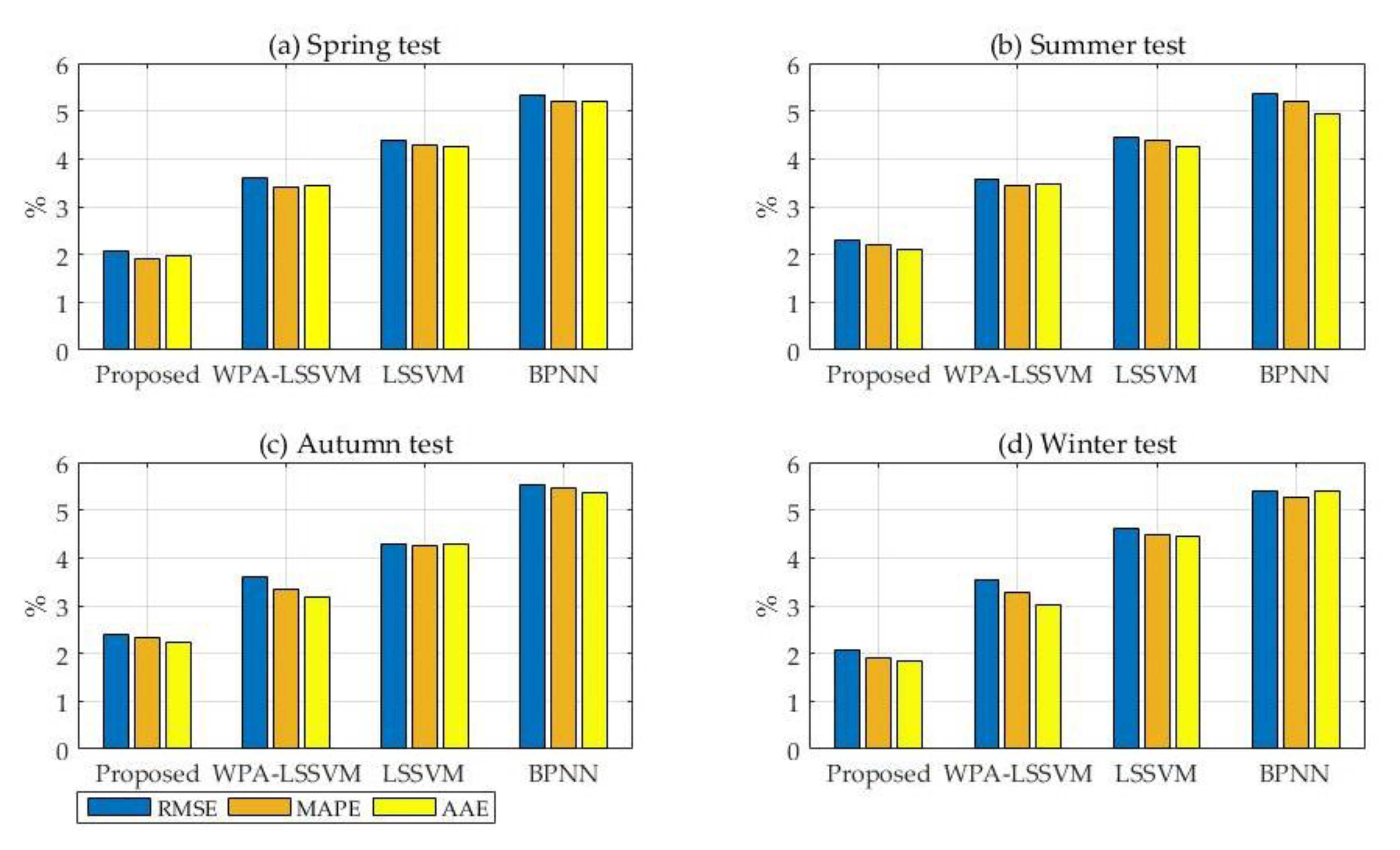
In order to further verify the validity of the proposed method, another e-bus charging station in Baoding, China, was selected for an experimental study. The load data of the station from January, 2016 to December, 2016 are provided in this paper, where seven successive days in each season were taken as test samples and the remaining data were used as training samples. The setting of parameters in WPA-LSSVM was consistent with the proposed method. In LSSVM, γ and σ2 were equal to 10.2801 and 11.2675, respectively. The values of the parameters in the BPNN model were same as those in the previous case study. Figure 12 displays the values of RMSE, MAPE and AAE.
From Figure 12, it can be seen that FC-WPA-LSSVM presents the lowest RMSE, MAPE and AAE, with corresponding values of 2.07%, 1.92% and 1.97 in the spring test, 2.29%, 2.20% and 2.11% in the summer test, 2.39%, 2.35% and 2.25% in the autumn test, and 2.08%, 1.90% and 1.84% in the winter test. It can be seen that the overall prediction performance of the forecasting approach was optimal due to the advantages of FC, WPA and LSSVM. In conclusion, the load forecasting model for e-bus charging stations based on FC-WPA-LSSVM can provide accurate data support for the economical operation of the station. In addition, the proposed model can also be applied to the load forecasting of other charging stations, and its prediction accuracy will not be affected by changes in the number of electric vehicles and other factors.
Since this forecasting model is based on MATLAB development, if the transportation company wants to use this model to predict the load in the future, they can also use it easily and obtain the forecast results without additional costs.
6. Conclusions
In view of the load characteristics for e-bus charging stations, this paper selected eight variables, including day type, maximum temperature, minimum temperature, weather condition, the number of accumulated daily number of charged e-buses and the loads at the same moment in the previous three days, as the input. A novel short-term load forecasting technique for e-bus charging stations based on FC-WPA-LSSVM was proposed, in which FC was used to extract similar dates as training samples, and WPA was introduced to optimize the parameters in LSSVM to improve the prediction accuracy. Two case studies were carried out to verify the developed approach in comparison with WPA-LSSVM, LSSVM and BPNN. The experimental results showed that the forecasting precision of the proposed model was better than the contrasting models. Hence, FC-WPA-LSSVM provides a new idea and reference for short-term load forecasting of e-bus charging stations.
The load of e-bus charging stations is a kind of power load with complex change rules and diverse influential factors. With the large-scale application of electric vehicles, more and more e-bus charging stations will start to be put into use. At that time, research on actual operation of charging stations will be more abundant. It is necessary to make further efforts to seek more suitable load forecasting approaches for e-bus charging stations based on the study of load variation rules and the internal relationships between the load and influential factors.
Funding
This work is supported by the Fundamental Research Funds for the Central Universities (Project No. 2018MS144).
Acknowledgments
Thanks for State Grid Hebei Electric Power Company providing the relevant data supporting.
Conflicts of Interest
The authors declare no conflict of interest.
References
- Tan, S.; Yang, J.; Yan, J.; Lee, C.; Hashim, H.; Chen, B. A Holistic low Carbon city Indicator Framework for Sustainable Development. Appl. Energy 2017, 185, 1919–1930. [Google Scholar] [CrossRef]
- Yan, J.; Chou, S.K.; Chen, B.; Sun, F.; Jia, H.; Yang, J. Clean, Affordable and Reliable Energy Systems for low Carbon city Transition. Appl. Energy 2017, 194, 305–309. [Google Scholar] [CrossRef]
- Majidpour, M.; Qiu, C.; Chu, P.; Pota, H.; Gadh, R. Forecasting the EV Charging load Based on Customer Profile or Station Measurement? Appl. Energy 2016, 163, 134–141. [Google Scholar] [CrossRef]
- Paparoditis, E.; Sapatinas, T. Short-Term Load Forecasting: The Similar Shape Functional Time-Series Predictor. IEEE Trans. Power Syst. 2013, 28, 3818–3825. [Google Scholar] [CrossRef] [Green Version]
- Yildiz, B.; Bilbao, J.I.; Sproul, A.B. A Review and Analysis of Regression and Machine Learning Models on Commercial Building Electricity load Forecasting. Renew. Sust. Energy Rev. 2017, 73, 1104–1122. [Google Scholar] [CrossRef]
- Cerne, G.; Dovzan, D.; Skrjanc, I. Short-term load forecasting by separating daily profile and using a single fuzzy model across the entire domain. IEEE Trans. Ind. Electron. 2018, 65, 7406–7415. [Google Scholar] [CrossRef]
- Ashtari, A.; Bibeau, E.; Shahidinejad, S.; Molinski, T. PEV Charging Profile Prediction and Analysis Based on Vehicle Usage Data. IEEE Trans. Smart Grid 2012, 3, 341–350. [Google Scholar] [CrossRef]
- Dai, Q.; Cai, T.; Duan, S.; Zhao, F. Stochastic Modeling and Forecasting of Load Demand for Electric Bus Battery-Swap Station. IEEE Trans. Power Deliv. 2014, 29, 1909–1917. [Google Scholar] [CrossRef]
- Tarsitano, A.; Amerise, I.L. Short-term load Forecasting Using a Two-Stage Sarimax Model. Energy 2017, 133, 108–114. [Google Scholar] [CrossRef]
- Zhang, W.G.; Xie, F.X.; Huang, M.; Juan, L.; Li, Y. Research on Short-Term Load Forecasting Methods of Electric Buses Charging Station. Power Syst. Prot. Control 2013, 41, 61–66. [Google Scholar]
- Xiao, L.; Shao, W.; Yu, M.; Ma, J.; Jin, C. Research and Application of a Hybrid Wavelet Neural Network Model with the Improved Cuckoo Search Algorithm for Electrical Power SYSTEM forecasting. Appl. Energy 2017, 198, 203–222. [Google Scholar] [CrossRef]
- Li, S.; Wang, P.; Goel, L. A Novel Wavelet-Based Ensemble Method for Short-Term Load Forecasting with Hybrid Neural Networks and Feature Selection. IEEE Trans. Power Syst. 2016, 31, 1788–1798. [Google Scholar] [CrossRef]
- Xiong, X.; Chen, L.; Liang, J. A New Framework of Vehicle Collision Prediction by Combining SVM and HMM. IEEE Trans. Intell. Transp. Syst. 2017, 19, 1–12. [Google Scholar] [CrossRef]
- Yang, Y.L.; Che, J.X.; Li, Y.Y.; Zhao, Y.J.; Zhu, S.L. An incremental electric load forecasting model based on support vector regression. Energy 2016, 113, 796–808. [Google Scholar] [CrossRef]
- Liu, W.; Xiaobo, X.U.; Xi, Z. Daily load forecasting based on SVM for electric bus charging station. Electr. Power Autom. Equip. 2014, 34, 41–47. [Google Scholar]
- Deo, R.C.; Kisi, O.; Singh, V.P. Drought forecasting in eastern Australia using multivariate adaptive regression spline, least square support vector machine and M5Tree model. Atmos. Res. 2017, 184, 149–175. [Google Scholar] [CrossRef] [Green Version]
- Lin, W.M.; Tu, C.S.; Yang, R.F.; Tsai, M.T. Particle swarm optimisation aided least-square support vector machine for load forecast with spikes. IET Gener. Trans. Distrib. 2016, 10, 1145–1153. [Google Scholar] [CrossRef]
- Li, C.; Li, S.; Liu, Y. A least squares support vector machine model optimized by moth-flame optimization algorithm for annual power load forecasting. Appl. Intell. 2016, 45, 1–13. [Google Scholar] [CrossRef]
- Liang, Y.; Niu, D.; Ye, M.; Hong, W.C. Short-Term Load Forecasting Based on Wavelet Transform and Least Squares Support Vector Machine Optimized by Improved Cuckoo Search. Energies 2016, 9, 827. [Google Scholar] [CrossRef]
- Padilha, C.A.D.A.; Barone, D.A.C.; Neto, A.D.D. A multi-level approach using genetic algorithms in an ensemble of Least Squares Support Vector Machines. Knowl.-Based Syst. 2016, 106, 85–95. [Google Scholar] [CrossRef]
- Dong, R.; Xu, J.; Lin, B. ROI-based study on impact factors of distributed PV projects by LSSVM-PSO. Energy 2017, 124, 336–349. [Google Scholar] [CrossRef]
- Sun, W.; Sun, J. Daily PM2.5 Concentration Prediction Based on Principal Component Analysis and LSSVM Optimized by cuckoo Search Algorithm. J. Environ. Manag. 2016, 188, 144. [Google Scholar] [CrossRef] [PubMed]
- Niu, D.; Liang, Y.; Wang, H.; Wang, M.; Hong, W.C. Icing Forecasting of Transmission Lines with a Modified Back Propagation Neural Network-Support Vector Machine-Extreme Learning Machine with Kernel (BPNN-SVM-KELM) Based on the Variance-Covariance Weight Determination Method. Energies 2017, 10, 1196. [Google Scholar] [CrossRef]
- Chen, X.; Tang, C.; Wang, J.; Zhang, L.; Liu, Y. A Novel Hybrid Based on Wolf Pack Algorithm and Differential Evolution Algorithm. Int. Symp. Comput. Intell. Des. 2017, 69–74. [Google Scholar] [CrossRef]
- Xue, B.; Zhang, M.; Browne, W.N.; Yao, X. A Survey on Evolutionary Computation Approaches to Feature Selection. IEEE Trans. Evolut. Comput. 2016, 20, 606–626. [Google Scholar] [CrossRef]
- Hassanpour, H.; Zehtabian, A.; Nazari, A.; Dehghan, H. Gender classification based on fuzzy clustering and principal component analysis. IET Comput. Vis. 2016, 10, 228–233. [Google Scholar] [CrossRef]
- Kumar, M.R.; Ghosh, S.; Das, S. Frequency dependent piecewise fractional-order modelling of ultracapacitors using hybrid optimization and fuzzy clustering. J. Power Sources 2016, 335, 98–104. [Google Scholar] [CrossRef]
- Alban, N.; Laurent, B.; Mitherand, N.; Ousman, B.; Martin, N.; Etienne, M. Robust and Fast Segmentation Based on Fuzzy Clustering Combined with Unsupervised Histogram Analysis. IEEE Intell. Syst. 2017, 32, 6–13. [Google Scholar] [CrossRef]
- Bai, X.; Wang, Y.; Liu, H.; Guo, S. Symmetry Information Based Fuzzy Clustering for Infrared Pedestrian Segmentation. IEEE Trans. Fuzzy Syst. 2017. [Google Scholar] [CrossRef]
- Zhu, B.; Han, D.; Wang, P. Forecasting carbon price using empirical mode decomposition and evolutionary least squares support vector regression. Appl. Energy 2017, 191, 521–530. [Google Scholar] [CrossRef]
- Yuan, X.; Tan, Q.; Lei, X.; Yuan, Y.; Wu, X. Wind Power Prediction Using Hybrid Autoregressive Fractionally Integrated Moving Average and Least Square Support Vector Machine. Energy 2017, 129, 122–137. [Google Scholar] [CrossRef]
- Niu, D.; Li, Y.; Dai, S.; Kang, H.; Xue, Z.; Jin, X.; Song, Y. Sustainability Evaluation of Power Grid Construction Projects Using Improved TOPSIS and Least Square Support Vector Machine with Modified Fly Optimization Algorithm. Sustainability 2018, 10, 231. [Google Scholar] [CrossRef]
- Niu, D.; Dai, S. A Short-Term Load Forecasting Model with a Modified Particle Swarm Optimization Algorithm and Least Squares Support Vector Machine Based on the Denoising Method of Empirical Mode Decomposition and Grey Relational Analysis. Energies 2017, 10. [Google Scholar] [CrossRef]
- Hu-Sheng, W.U.; Zhang, F.M.; Lu-Shan, W.U. New swarm intelligence algorithm—Wolf pack algorithm. Syst. Eng. Electr. 2013, 35. [Google Scholar] [CrossRef]
- Wu, H.S.; Zhang, F.M. Wolf Pack Algorithm for Unconstrained Global Optimization. Math. Probl. Eng. 2014, 1, 1–17. [Google Scholar] [CrossRef]
- Li, C.M.; Du, Y.C.; Wu, J.X.; Lin, C.H.; Ho, Y.R.; Lin, Y.J.; Chen, T. Synchronizing chaotification with support vector machine and wolf pack search algorithm for estimation of peripheral vascular occlusion in diabetes mellitus. Biomed. Signal Process. Control 2014, 9, 45–55. [Google Scholar] [CrossRef]
- Mustaffa, Z.; Sulaiman, M.H. Price predictive analysis mechanism utilizing grey wolf optimizer-Least Squares Support Vector Machines. J. Eng. Appl. Sci. 2015, 10, 17486–17491. [Google Scholar]
- Li, X.; Lu, J.H.; Ding, L.; Xu, G.; Li, J. In Building Cooling Load Forecasting Model Based on LS-SVM. In Proceedings of the IEEE Internatonal Asia-Pacific Conference on Information Processing, Shenzhen, China, 18–19 July 2009. [Google Scholar]
- Bin, H.; Zu, Y.X.; Zhang, C. A Forecasting Method of Short-Term Electric Power Load Based on BP Neural Network. Appl. Mech. Mater. 2014, 538, 247–250. [Google Scholar] [CrossRef]
Figure 1.
Typical daily load curve of an e-bus charging station in Baoding.

Figure 2.
The relationship between meteorological conditions and power load. (a) the highest temperature and load; (b) the weather and load; (c) the average wind speed and load; (d) the average humidity and load.
Figure 2.
The relationship between meteorological conditions and power load. (a) the highest temperature and load; (b) the weather and load; (c) the average wind speed and load; (d) the average humidity and load.

Figure 3.
Relationship between temperature and daily load.

Figure 4.
Relationship between weather conditions and daily load.

Figure 5.
Bionic graph of WPA.

Figure 6.
The flow chart of the proposed forecasting model.

Figure 7.
Forecasting results of the proposed model.

Figure 8.
The RE of the proposed model.

Figure 9.
Forecasting results: (a) forecasting results of Spring test; (b) forecasting results of Summer test; (c) forecasting results of Autumn test; (d) forecasting results of Winter test.
Figure 9.
Forecasting results: (a) forecasting results of Spring test; (b) forecasting results of Summer test; (c) forecasting results of Autumn test; (d) forecasting results of Winter test.

Figure 10.
RE of forecasting approaches: (a) RE of Spring test; (b) RE of Summer test; (c) RE of Autumn test; (d) RE of Winter test.
Figure 10.
RE of forecasting approaches: (a) RE of Spring test; (b) RE of Summer test; (c) RE of Autumn test; (d) RE of Winter test.

Figure 11.
RMSE, MAPE and AAE of the forecasting results (I).

Figure 12.
RMSE, MAPE and AAE of the forecasting results (II): (a) Spring test; (b) Summer test; (c) Autumn test; (d) Winter test.
Figure 12.
RMSE, MAPE and AAE of the forecasting results (II): (a) Spring test; (b) Summer test; (c) Autumn test; (d) Winter test.


Table 1.
Load characteristics of different day types.
| Day Type | Annual Average Daily Maximum Load/kW | Annual Average Daily Average Load/kW |
|---|---|---|
| Monday | 669.16 | 386.70 |
| Tuesday | 663.28 | 377.07 |
| Wednesday | 649.63 | 376.95 |
| Thursday | 647.03 | 366.23 |
| Friday | 636.54 | 370.55 |
| Saturday | 573.46 | 338.97 |
| Sunday | 590.45 | 349.94 |
© 2018 by the author. Licensee MDPI, Basel, Switzerland. This article is an open access article distributed under the terms and conditions of the Creative Commons Attribution (CC BY) license (http://creativecommons.org/licenses/by/4.0/).
Share and Cite
MDPI and ACS Style
Zhang, X. Short-Term Load Forecasting for Electric Bus Charging Stations Based on Fuzzy Clustering and Least Squares Support Vector Machine Optimized by Wolf Pack Algorithm. Energies 2018, 11, 1449. https://doi.org/10.3390/en11061449
AMA Style
Zhang X. Short-Term Load Forecasting for Electric Bus Charging Stations Based on Fuzzy Clustering and Least Squares Support Vector Machine Optimized by Wolf Pack Algorithm. Energies. 2018; 11(6):1449. https://doi.org/10.3390/en11061449
Chicago/Turabian StyleZhang, Xing. 2018. "Short-Term Load Forecasting for Electric Bus Charging Stations Based on Fuzzy Clustering and Least Squares Support Vector Machine Optimized by Wolf Pack Algorithm" Energies 11, no. 6: 1449. https://doi.org/10.3390/en11061449
Note that from the first issue of 2016, this journal uses article numbers instead of page numbers. See further details here.