Improving Short-Term Heat Load Forecasts with Calendar and Holiday Data


1
Department of Engineering, Aarhus University, Inge Lehmanns Gade 10, 8000 Aarhus, Denmark
2
AffaldVarme Aarhus, Municipality of Aarhus, Bautavej 1, 8210 Aarhus, Denmark
3
Department of Physics and Astronomy, Aarhus University, Ny Munkegade 120, 8000 Aarhus, Denmark
*
Author to whom correspondence should be addressed.
Energies 2018, 11(7), 1678; https://doi.org/10.3390/en11071678
Submission received: 28 May 2018
/
Revised: 21 June 2018
/
Accepted: 25 June 2018
/
Published: 27 June 2018
(This article belongs to the Special Issue Short-Term Load Forecasting by Artificial Intelligent Technologies)
Abstract
:The heat load in district heating systems is affected by the weather and by human behavior, and special consumption patterns are observed around holidays. This study employs a top-down approach to heat load forecasting using meteorological data and new untraditional data types such as school holidays. Three different machine learning models are benchmarked for forecasting the aggregated heat load of the large district heating system of Aarhus, Denmark. The models are trained on six years of measured hourly heat load data and a blind year of test data is withheld until the final testing of the forecasting capabilities of the models. In this final test, weather forecasts from the Danish Meteorological Institute are used to measure the performance of the heat load forecasts under realistic operational conditions. We demonstrate models with forecasting performance that can match state-of-the-art commercial software and explore the benefit of including local holiday data to improve forecasting accuracy. The best forecasting performance is achieved with a support vector regression on weather, calendar, and holiday data, yielding a mean absolute percentage error of 6.4% on the 15–38 h horizon. On average, the forecasts could be improved slightly by including local holiday data. On holidays, this performance improvement was more significant.
1. Introduction
Energy systems are changing throughout the world, and heat load forecasting is gaining importance in modern district heating systems [1]. The growing penetration of renewable energy sources makes energy production fluctuate beyond human control and increases the volatility in electricity markets. Stronger coupling between the heating and electricity sectors means that production planners in systems with combined heat and power generation need accurate heat load forecasts in order to optimize the production.
It is not trivial to forecast district heating demand on time scales that are relevant for trading on the day-ahead electricity market. The total heat load in a district heating system is influenced by several factors—most importantly, the weather, the building mass of the city, and the behavior of the heat consumers. Cold and windy weather increases the heat demand, and warm and sunny weather decreases it. The constitution of the building mass influences how the heat load responds to changes in the weather [2]. Human behavior is an often overlooked factor, and, especially in summer, the heat demand is dominated by hot water consumption rather than space heating. Consumer behavior can vary considerably from day to day, and the heat load on special occasions, e.g., New Year’s Eve, is notoriously difficult to forecast accurately.
Heat load forecasting has been studied extensively in the scientific literature. The successful application of simple linear models in [3,4] has inspired us to use an ordinary least squares (OLS) model as a simple benchmarking model. Statistical time-series models, such as SARIMA (seasonal autoregressive integrated moving average) models [4,5] and grey-box models combining physical insight with statistical modeling [6], are natural ways of handling the temporal nature of load forecasting. These models are usually linear and struggle with multiple seasonality. In [7], the authors compared a number of machine learning algorithms, including a simple feed forward neural network, support vector regression (SVR), and OLS. They concluded that the SVR model performs best. The strong forecasting capabilities of SVR models have also been demonstrated in [8], where heat demand was forecasted based on natural gas consumption. Neural networks have been widely applied in load forecasting. Several studies apply simple feed forward networks with one hidden layer such as the multilayer perceptron (MLP) [7,9,10]. A recurrent neural network is used in [11] to better handle non-stationarities in the heat load. A comprehensive review of load forecasting in districts can be found in [1].
In the present study, we chose to compare three different machine learning models: OLS, MLP, and SVR, as they have all proven effective for heat load forecasting. Some studies attempt to include the different consumer behavior on weekdays and weekends. Working days and non-working days are modeled with distinct profiles in [12], and in [4] mid-week holidays were treated as Saturdays or Sundays. In [13], the correlation between electric load and weather variables was exploited to forecast the aggregated load using MLP models, and the authors explored the different autocorrelations of the load on weekdays and weekends. In this study, we include generic calendar data such as the day of the week, as well as local holiday data to account for observances, national holidays, and city-specific holidays, i.e., school holidays.
School holidays are often planned locally, and some religious holidays, e.g., Easter, fall on different dates each year. Therefore, generic calendar data is insufficient for modeling events that depend on local holidays. Heat consumers behave differently on holidays and change the pattern of consumption, so including local holiday data in heat load forecast models has the potential to improve forecast accuracy.
The novelty of this work lies in the application of new data sources, specifically local holiday data, to create heat load forecasting models that more accurately capture consumer behavior. To the best of our knowledge, school holiday data has not previously been used for heat load forecasting. We isolate the effect of using local holiday data by employing machine learning models that have proven effective for heat load forecasting in the past. Moreover, we base our modeling on a very large amount of data. Seven years of hourly heat load and weather data supplemented with data about national holidays, observances, and school holidays help the forecast models capture rare load events.
The remainder of the paper is structured as follows. The Methodology section describes the data foundation, the machine learning models, and the validation and testing procedure. In the Results section, the forecasting models are benchmarked and compared, and the potential of using new data sources is evaluated. The paper is wrapped up in the Conclusion section.
2. Methodology
In this section, we describe the data foundation and how the heat load forecasting models were built, validated and tested.
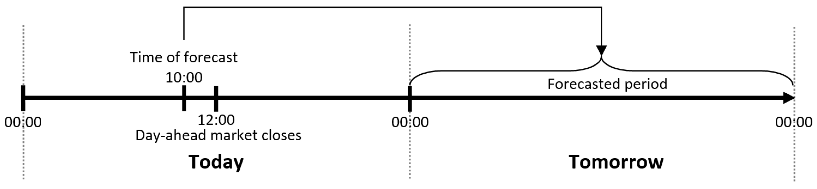
The focus of this paper is to create heat load forecasts that are relevant on the time horizon of the day-ahead electricity market. Therefore, a forecast must be produced each morning at 10:00 for each hour of the following day. This timeline, illustrated in Figure 1, allows time for communication between different actors in a production system and for planning of the following day’s heat production in accordance with the bids in the day-ahead electricity market.
The analysis in this paper is based on seven years of data for the total hourly heat load of Aarhus, Denmark. The years 2009, 2010, 2012, 2013, 2014, 2015, and 2016 were used. Unfortunately, heat load data from 2011 has not been available to us. We denote the heat load in hour t by .
2.1. Weather Data
The heat demand depends strongly on the weather. Hourly outdoor temperature, wind speed, and solar irradiation for the seven years were obtained from [14]. Weather data from the geographical point N 56°2′42.24″, E 9°59′59.95″ in the southern part of Aarhus was used. Weather forecasts of the outdoor temperature, wind speed, and solar irradiation were provided by the Danish Meteorological Institute (DMI) and used to test the performance of the heat load forecasts as realistically as possible. These weather forecasts were based on the HIRLAM (High Resolution Limited Area Model), a numerical weather prediction system developed by a consortium of European meteorological institutes with the purpose of providing state-of-the-art short-range weather predictions [15], for numerical weather prediction, had a forecast horizon of up to 54 h, and were disseminated four times a day [15]. We denote the outdoor temperature, wind speed, and solar irradiance by , and , respectively.
2.2. Calendar Data
The heat demand has a strong social component that depends on human behavior. The social component is part of the reason for the daily and weekly patterns in the heat load. Different load profiles on weekdays and weekends can also be explained by consumer behavior. In order to allow the forecast models to account for load variations that are tied to specific days, seasons, and times of day, certain calendar data were included as input variables. Specifically, the hour of the day, the day of the week, the weekend, and the month of the year were used as input. How the calendar data was encoded and included in the models is described in Section 2.4.1.
2.3. Holiday Data
In addition to generic calendar data, we also used more specific local data about special days that may influence the heat consumption pattern. The district heating system of Aarhus, Denmark, served as our case study. Therefore, we used data about Danish national holidays, observances, and local school holidays. National holidays and observances were sourced from [16]. National holidays include New Year’s Day, Christmas Day, Easter Day, etc. and constitute 11 days per year. Observances include, e.g., Christmas Eve and Constitution Day and amount to six days per year. Information about the municipal school holidays was collected from local schools in the Aarhus area and amounts to 96 days per year on average. Note that all national holidays are also school holidays. It is clear that this kind of information is highly local and that gathering such data, compared to the generic calendar data, is more difficult. The following analysis will illuminate whether including this data significantly improves heat load forecasts, or if more easily available data types are sufficient.
2.4. Data Exploration
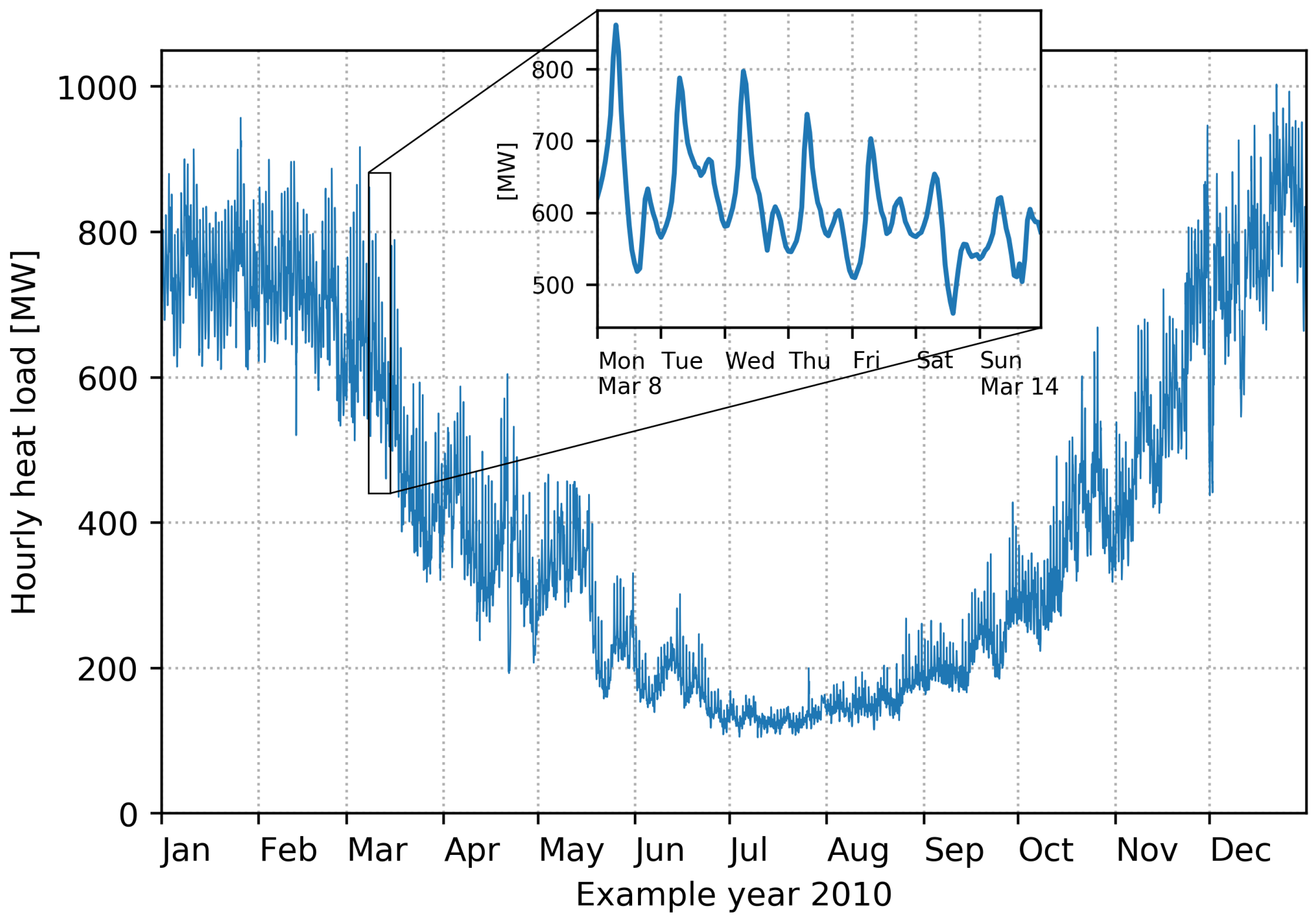
Figure 2 shows the average hourly heat load for the example year of 2010. Notice how much the heat load varies over the year both in magnitude and in variance. The zoomed inset in the plot shows the heat load variations over a week in March. A clear daily pattern can be observed, with a sharp morning peak between 7:00 and 8:00 on weekday mornings. The morning peak is a well-known phenomenon in the district heating community and is caused by many people showering around the same time every morning. On weekends, morning peaks can be observed later in the morning and tend to be less sharp compared to weekdays. From the inset, it is clear that the daily load pattern varies substantially within just one week.
The heat demand has peaks in its autocorrelation function at 24 h, 48 h, 72 h, and so on. This is due to the strong daily pattern. There is also a notable peak at 168 h (one week). In order to capture this behavior, lagged values of the heat load were used as input variables in the modeling. Specifically, we included the heat load lagged with 24 h, 48 h, and 168 h. Looking at Figure 1, we see that the forecast horizon varies between 15 h and 38 h. The heat load in the first hour of the day can be forecasted with the shortest horizon, and the last hour of each day is forecasted with the longest horizon. When forecasting hours with a forecast horizon of 24 h or less, the heat load lagged 24 h can be used. When forecasting hours with a longer horizon than 24 h, the heat load lagged with 48 h must be used instead. A power spectrum analysis confirmed strong peaks at frequencies 1/12 h−1 and 1/24 −1, but 12 h is shorter than the shortest forecast horizon and was thus discarded. The two lags that best captured the daily and weekly pattern of the heat load were included. We denote the lagged heat load by , , and , respectively.
The most important weather variable when modeling district heating loads is the outdoor temperature, because there is a strong negative correlation between the heat demand and the outdoor temperature. Depending on the specific district heating system, solar irradiation and wind speed can also be significant predictors for the heat load [2]. Due to the thermal mass of the buildings in a district heating system, there is a certain inertia in the heat load when changes in the weather occur. On the individual building level, this inertia is handled in great detail in the civil engineering literature [17]. Since we were forecasting the heat load of an entire city, we took a more simplified approach. In the Aarhus district heating system, the heat load is most strongly correlated with the outdoor temperature lagged by 4 h, compared to other time lags of the temperature. The heat load also correlates most strongly with the solar irradiation lagged by 4 h. There seemed to be no benefit in lagging the wind speed. Only including two specific lags, is of course a simplification of the dynamics of the system, but the results of including them were significantly better than just using simultaneous (lag 0 h) weather variables. Summing up, the following five weather variables were included in the modeling: , , , , and .
Outdoor temperature and, as a consequence, the heat load varies substantially from year to year [18]. The mean annual temperatures in our dataset spanned a range of 2.5 °C. Compared to the mean load of the whole dataset (excluding 2016), the annual mean heat load was 15% higher in the coldest year and 11% lower in the warmest year.
2.4.1. Data Scenarios and Pre-Processing
In order to evaluate the effect of including the various types of input data for forecasting heat load, three different data scenarios have been defined. We call these scenarios: “Only Weather Data,” “Weather and Calendar,” and “Weather, Calendar, and Holidays”. Table 1 details the input data used in each scenario.
To achieve the best performance of the models, the input data were scaled and encoded as follows. All the continuous variables (lagged heat load and weather) were standardized to have mean 0 and standard deviation 1. The calendar data and holiday data were included as so-called dummy variables. Dummy variables are a way to represent categorical variables as binary variables. For instance, whether or not a given hour falls on a school holiday can be encoded as a binary variable (0 or 1). The day of week can be encoded as six binary variables: one variable indicating if it is Monday, one indicating if it Tuesday, etc. Only six variables are needed to encode seven days, because if it is not any of the days from Monday to Saturday, then it must be Sunday. Using similar dummy variables all the calendar and holiday data was included. Encoding categorical data as dummy variables is a standard machine learning method [19].
2.5. Machine Learning Models
We benchmarked and compared three different machine learning models that have all previously been proven adequate for heating load forecasting [7,8]: ordinary least squares regression, multilayer perceptron, and support vector regression.
2.5.1. OLS—Ordinary Least Squares Regression
Ordinary least squares regression is a simple model type in which the output is modeled with the hyperplane that minimizes the squared residuals between the target and the output of the model. Sometimes referred to as multiple linear regression, it is a popular model due to its simplicity, computational speed, and the fact that results can be easily interpreted. Because of its linear structure, the OLS model underperforms when modeling nonlinear input–output relationships.
2.5.2. MLP—Multilayer Perceptron
A multilayer perceptron is a simple kind of neural network. Neural networks have been applied to problems in many fields, including heat load forecasting, due to their ability to capture complicated relationships between input and output [7,9,11]. A multilayer perceptron has at least one hidden layer between the input and output layers of the model and a nonlinear activation function allows the model to capture nonlinear relationships between input and output. A good coverage of neural network models and the multilayer perceptron can be found in [20]. We used a multilayer perceptron with one hidden layer and the rectifier activation function: . We have experimented with adding more hidden layers, but the increase in the model accuracy was not large enough to justify the growth in model complexity and the risk of overfitting.
Besides the simple multilayer perceptron, we have experimented with a more advanced type of neural network. Recurrent neural networks with long short-term memory (LSTM) units [21] were implemented in an attempt to simplify the feature selection and leave it to the model to discover relevant lags of heat load and weather data. Our initial LSTM networks yielded results comparable to the simpler models included in this work, but their performance tended to be inconsistent. The benefit of simplified feature selection may also be outweighed by a more complicated model selection and training procedure. The LSTM modeling for heat load forecasting requires more work and will be left for future work.
2.5.3. SVR—Support Vector Regression
Support vector regression is the application of support vector machine models to regression problems and was first introduced in [22]. Support vector regression has a computational advantage in very high dimensional feature spaces. The model only depends on a subset of input data, because it minimizes a cost function that is insensitive to points within a certain distance from the prediction. The cost function is less sensitive to small errors and less sensitive to very large errors and outliers, compared to the quadratic cost function minimized in the ordinary least squares regression. To avoid overfitting, the model is governed by a regularization parameter C, that ensures that the parameters of the model do not grow uncontrollably. The smaller the value of C, the harder large model parameters are penalized. Support vector regression is explained in great detail in [19,20]. By employing the so-called “kernel trick”, support vector regression can handle nonlinear input–output relationships. A very popular kernel function is the radial basis function kernel (RBF), which has been proven effective in this application as well. The RBF kernel is governed by a kernel parameter . The greater the value of , the more prone the model is to overfitting, but if is chosen too small, the model may be underfitting and fail to capture actual input–output relationships.
Summing up, the three machine learning models OLS, MLP, and SVR were chosen because they have all been successfully applied to heat load forecasting in the past. Using well-established algorithms allows us to focus on the main research question: whether conventional heat load forecasts can be improved by adding new types of data. Each of the models have advantages and disadvantages. The advantage of the OLS model is that it is computationally cheap, and its estimated parameters carry a physical interpretation. The disadvantage is that the model is linear and fails to capture nonlinearities in input–output relationships. The advantage of the MLP model is that it is capable of capturing very complex relationships between input and output. A disadvantage of neural network models, such as MLP, is the risk of overfitting and that they require careful tuning of several hyperparameters. Finally, the SVR model has the advantage of being robust to outliers and that the final model depends only on a subset of the training data. The SVR model, however, is sensitive to the scaling of the input data and the correct tuning of regularization and kernel parameters.
2.6. Model Selection and Testing
A good forecast model is one that performs well on previously unseen data. This is the generalization ability of the model. In order to accurately measure the generalization performance of the models, we divided the full dataset (seven years of hourly data) into a training and validation set and a test set. All model selection and training was performed on the years from 2009 to 2015 (2011 not included). This is the training and validation set. The entire year of 2016 was used as a blind test set to estimate the generalization performance of the forecasts.
The three models were chosen and their hyperparameters tuned based on sixfold cross-validation on the years 2009, 2010, 2012, 2013, 2014, and 2015. Using six folds ensured that each fold contained an entire year and thus represented the full annual variation of the heat load. In the cross-validation, the different models and data scenarios were scored according to the hourly root mean square error (RMSE)
where is the forecasted heat load for hour t, and N is the number of hours.
The OLS model does not have any hyperparameters to tune, but a model with a nonzero constant term was chosen. In the MLP model, we tuned the number of neurons in the hidden layer using a grid search on the cross-validation scores. A MLP model with one hidden layer consisting of 110 hidden neurons was chosen, and the L2 regularization parameter was set to 0.1. In the SVR model, the best choices for the regularization parameter and the kernel parameter were found to be and . All modeling has been performed in Python 2.7 using the scikit-learn framework (version 0.19.0) [23].
All results presented in the following section were produced using the blind test year 2016. This year was not used for any of the training, data exploration, or model selection. In the Results section, we employ two other forecast error metrics, in addition to the RMSE. The mean absolute error (MAE) is also an absolute error metric (here in units of MW), but it is less sensitive to large errors, compared to the RMSE. The MAE is defined as
Finally, we use the relative error metric mean absolute percentage error (MAPE) to facilitate easier comparison between different district heating systems. The MAPE is defined as
3. Results
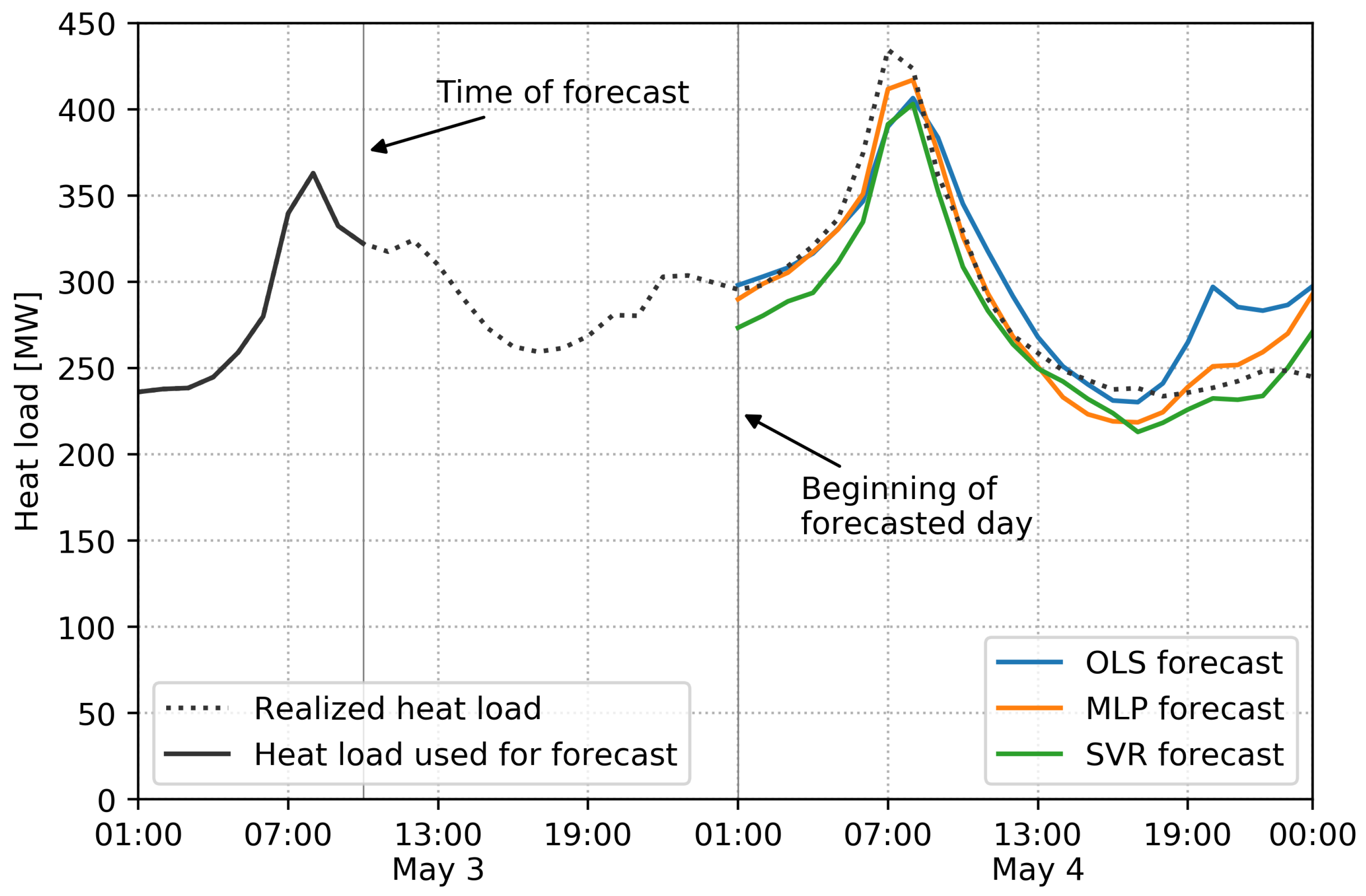
The heat load in a district heating system has been forecasted using three different machine learning models, described in the previous section: OLS, MLP, and SVR. The performance of these models have been tested by letting them produce a forecast for the following day using the input data available each day at 10:00 a.m.The models have been trained exclusively on data prior to the test year 2016 to be able to accurately gauge their generalization performance. Figure 3 shows an example of the forecasts produced for 4 May. Only the heat load up to the time of the forecast was used as input to produce the forecast. Real weather forecasts were used as weather inputs for 4 May, as opposed to the historical weather data used for training. It is clear how the three forecast models produce similar, yet distinct forecasts. On 4 May, the MLP model appears to produce the best forecast, especially in the morning.
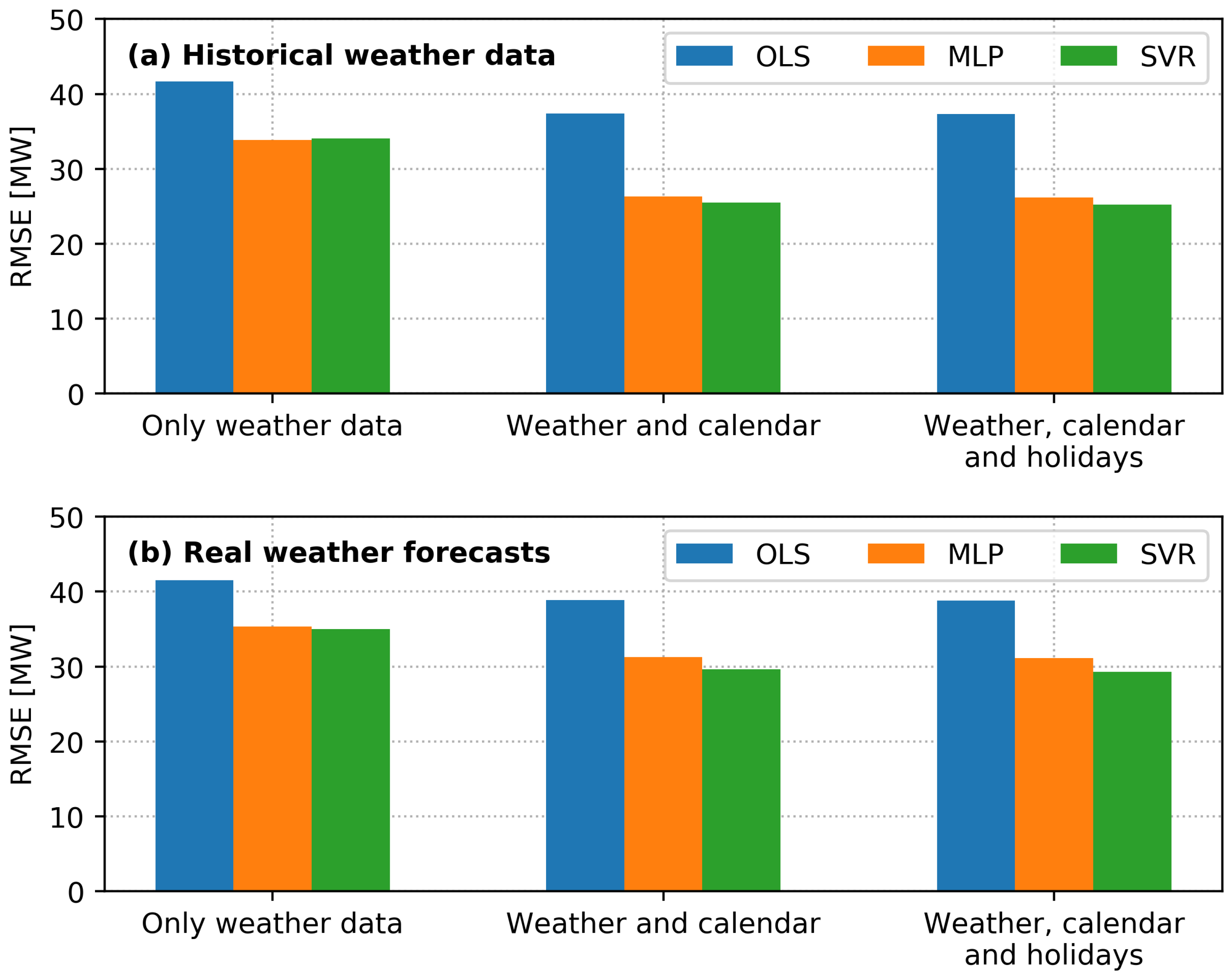
Figure 4 summarizes the performance of the three models in the three different data scenarios. The top panel shows the forecast performance that could be achieved if weather forecasts were 100% accurate, simulated by using historical weather data. The bottom panel shows the performance using real weather forecasts. Comparing the three data scenarios, we see the benefit of including different data types in the modeling. In the first scenario, only lagged heat load and weather data are used as input. In the second scenario, generic calendar data is included as well, and in the third scenario, local observances, national holidays, and school holidays are also included as inputs to the model. Including calendar data significantly improves performance, compared to only using weather data. Extending the input data with holiday data as well results in an additional, but small improvement compared to using generic calendar data only. Obtaining the local holiday data can be laborious or impossible, so it is positive to see generic calendar data yielding comparable results. It is much easier to apply these models to a wide range of district heating systems around the world if it can be done without collecting local holiday data.
Figure 4 allows for comparison of the performance of the three machine learning models as well. The OLS model stands out by performing significantly worse than the other two models in all scenarios. The OLS model has a root mean square error of 38.9 MW, compared to 31.1 MW and 29.3 MW for the other two models when using real weather forecasts, calendar, and holiday data (bottom panel). The poor performance of the OLS model can be attributed to its linear structure. The relationship between the outdoor temperature and the heat load in a temperate climate is nonlinear. This causes the linear model to perform poorly during summer by undershooting the heat load and overestimating its variance. The two nonlinear models, MLP and SVR, perform similarly in these scenarios. The SVR model has the smallest error, and the focus in the rest of this paper will be on the SVR model using weather, calendar, and holiday data.
3.1. The Value of Improving Weather Forecasts
Figure 4 has two panels. The top panel shows the forecast errors that could be achieved if weather forecasts predicted the measured weather completely accurately. This has been simulated by allowing the models to use actual measured weather data, instead of weather forecasts as input when producing the load forecast. The top panel reflects the scenario in the which future weather is known. The bottom panel shows the results in the case where real forecast data has been used instead. This is the actual forecast performance that can be achieved in an operational situation, given the current quality of weather forecasts. Having access to weather forecasts without prediction errors could, in a perfect world, reduce the error from 29.3 MW to 25.2 MW in the forecasts from the best model. While an error reduction of 4.1 MW is a start, perfecting the weather forecast only shaves 14% off the error. The remainder of the load forecast error has other causes than weather forecast errors, a result that was also found in [24], where ensemble weather predictions were used to quantify heat load forecasting uncertainty.
The OLS model using only weather data and lagged heat load does not perform notably different on historical weather data compared to real weather forecasts. This can be explained by the OLS model attributing greater weight to the lagged heat load compared to the weather, because the relationship between the heat load and the weather is nonlinear.
The forecast performance, shown in the top of Figure 4, is similar to the performance that was achieved during training and cross-validation. This indicates that the models have not been overfitted and generalize well to out-of-sample predictions.
It is worth pointing out that the performance of all these models, even the OLS model using only weather data, exceeds the performance of the commercial forecasting system that is currently in operation in the Aarhus district heating system. This commercial forecasting system had an RMSE of 41.9 MW in year of 2016 on the same forecast horizons. In relative terms, the SVR model has a MAPE of 6.4% versus 8.3% for the commercial system. The models presented here perform better than all other forecast models that have been used in the Aarhus district heating system.
3.2. Seasonal Performance Variations
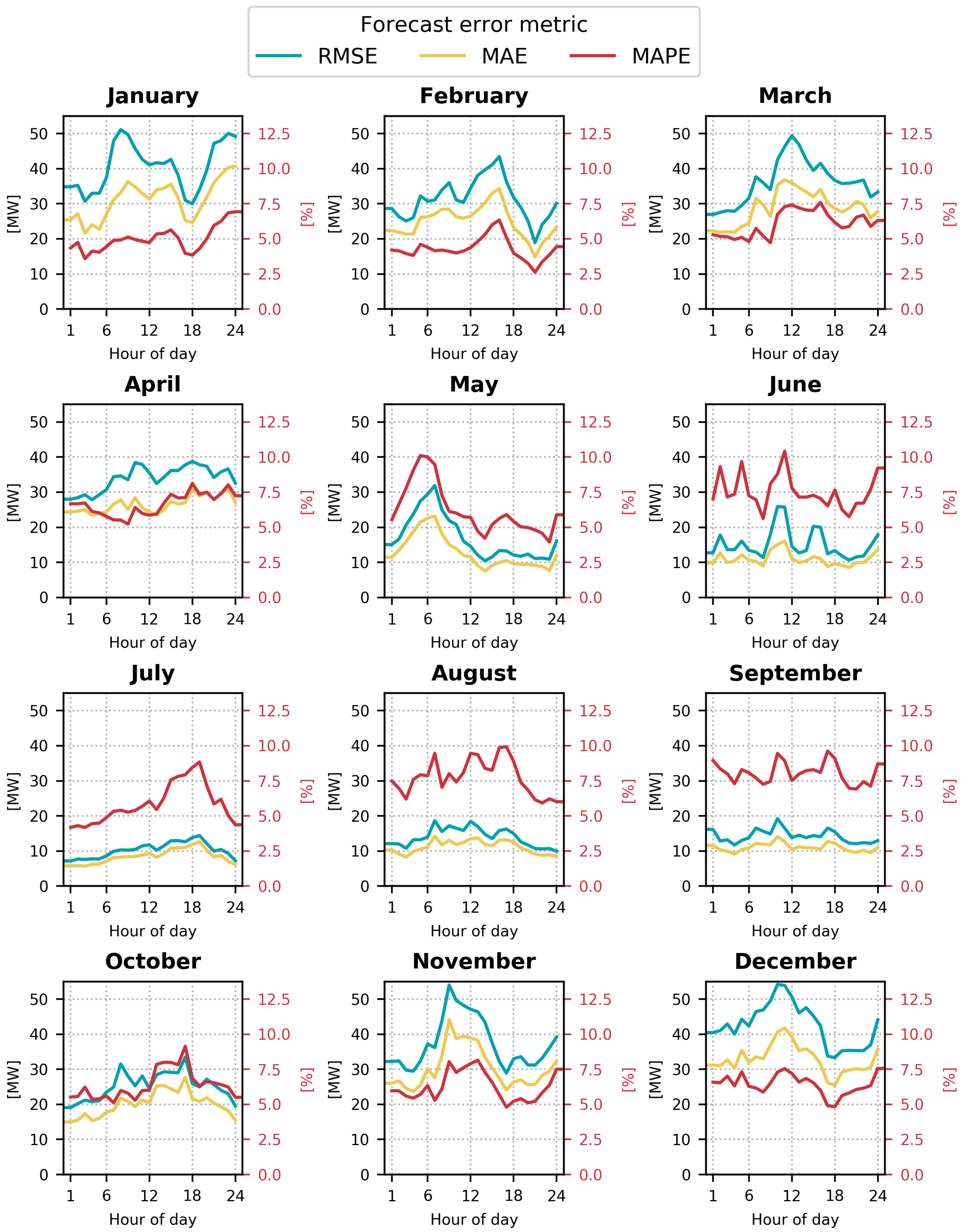
The heat load varies significantly over the year, both in magnitude and in variance, as exemplified in Figure 2. It can be a challenge for a single model to adequately forecast both winter and summer heat loads. Therefore, it is relevant to further investigate the model performance throughout the year. The forecast error of the best model, SVR using weather, calendar, and holiday data, is illustrated in Figure 5. Three different error metrics are shown: on the left axes, the RMSE (blue) and MAE (yellow) are shown in MW; on the right axes, the MAPE (red) is shown in percent. The horizontal axes show the hour of day for the forecasted hour, and each subplot depicts a month in the year. This makes it possible to see if it is harder to forecast the morning peak and if the forecast horizon impacts the accuracy. Keep in mind that Hour 1 has the shortest forecast horizon (15 h), and Hour 24 has the longest horizon (38 h), since the forecasts are produced at 10:00 a.m. the previous day.
Inspecting Figure 5, it is clear that the absolute error measures RMSE and MAE are largest in winter and smallest in summer. This is a reflection of the annual heat load profile and the large load with large variance during winter. In late fall and winter, the RMSE can be above 50 MW in some hours, whereas it can be below 10 MW in some hours in July. The relative error metric MAPE behaves in the opposite way. The relative error is smaller in the winter months and larger in summer months, but it stays between 2.5% and 10.5%. This is a consequence of the annual load variations being larger than the annual variations in the absolute error.
There is no clear pattern in the way the error changes during the day. The model does not seem to perform worse between 7:00 and 8:00 in the morning, where the morning peak falls. November and May are exceptions to this rule. In many applications, the error of a forecast model increases with the forecast horizon (here the hour of day). We do not observe a general increasing trend in the error with the hour of day. This indicates that the weather forecasts that are used as inputs to create the forecast are not significantly worse at the longest horizon compared to the shortest horizon. It may also be due to weather forecasting accuracy having a minor impact on the heat load forecasting error, as we saw from Figure 4. If we were to increase the forecast horizon further, the forecast error would most likely increase.
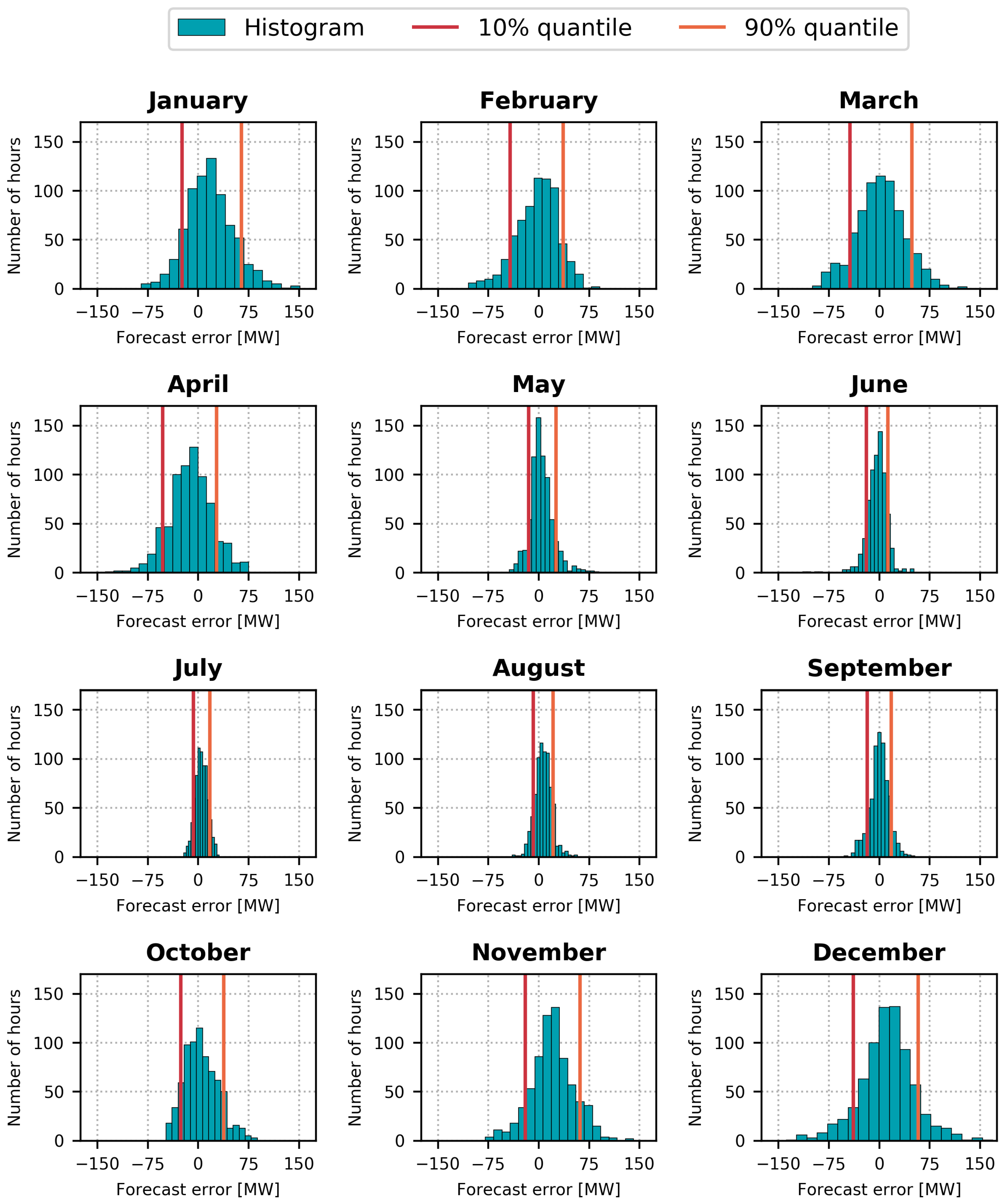
The forecast error varies significantly over the year, but aggregated error metrics such as RMSE, MAE, or MAPE do not tell the full story. Maximum errors can be relevant for unit commitment in the production planning and for evaluating risk regarding trading in the electricity market. Figure 6 shows histograms for the hourly error for each month of the blind test year 2016. The 10% and 90% quantiles have been indicated in each plot. It is clear that the width of the error distribution varies substantially from month to month. During the summer, the forecast error is quite confined, but the distribution widens in late fall and becomes widest in December.
In Table 2, a summary of the error distribution is shown. The 99% and 1% quantiles of the error distribution are indications of the maximum errors that can be expected. Ninety-eight percent of the forecasted hours have forecast errors between the 1% and the 99% quantile. The best month is July with 98% of the errors falling between −16.0 and 25.8 MW. The worst month is December, where there is a 1% risk of the forecast overshooting by more than 115.0 MW and a 1% risk of the forecast being more than 96.7 MW too low. These extreme errors can approach 20% of the mean heat load in December.
From the histograms in Figure 6, it is also clear that the error distributions are not completely symmetric around 0. In January, for instance, the distribution is shifted slightly to the positive, and in April it is shifted to the negative side. The forecast appears to be biased differently in different months. The mean error for each month (ME) is shown in Table 2. The bias can be as large as 20.5 MW, with November being the worst month. September performs the best with a mean error of merely 0.3 MW. Varying monthly biases could be remedied by training separate models for each month. However, the focus in this paper is to investigate the effects of including holiday data to model human behavior, and training monthly forecast models would obscure the effects of using holiday data. There is also the possibility that the weather forecasts perform differently at different times of year.
In conclusion, there are significant seasonal variations in the performance of the best heat load forecast. The absolute errors are largest in winter and smallest in summer, with December being the hardest month to forecast and July being the easiest.
3.3. The Value of Calendar and Holiday Data
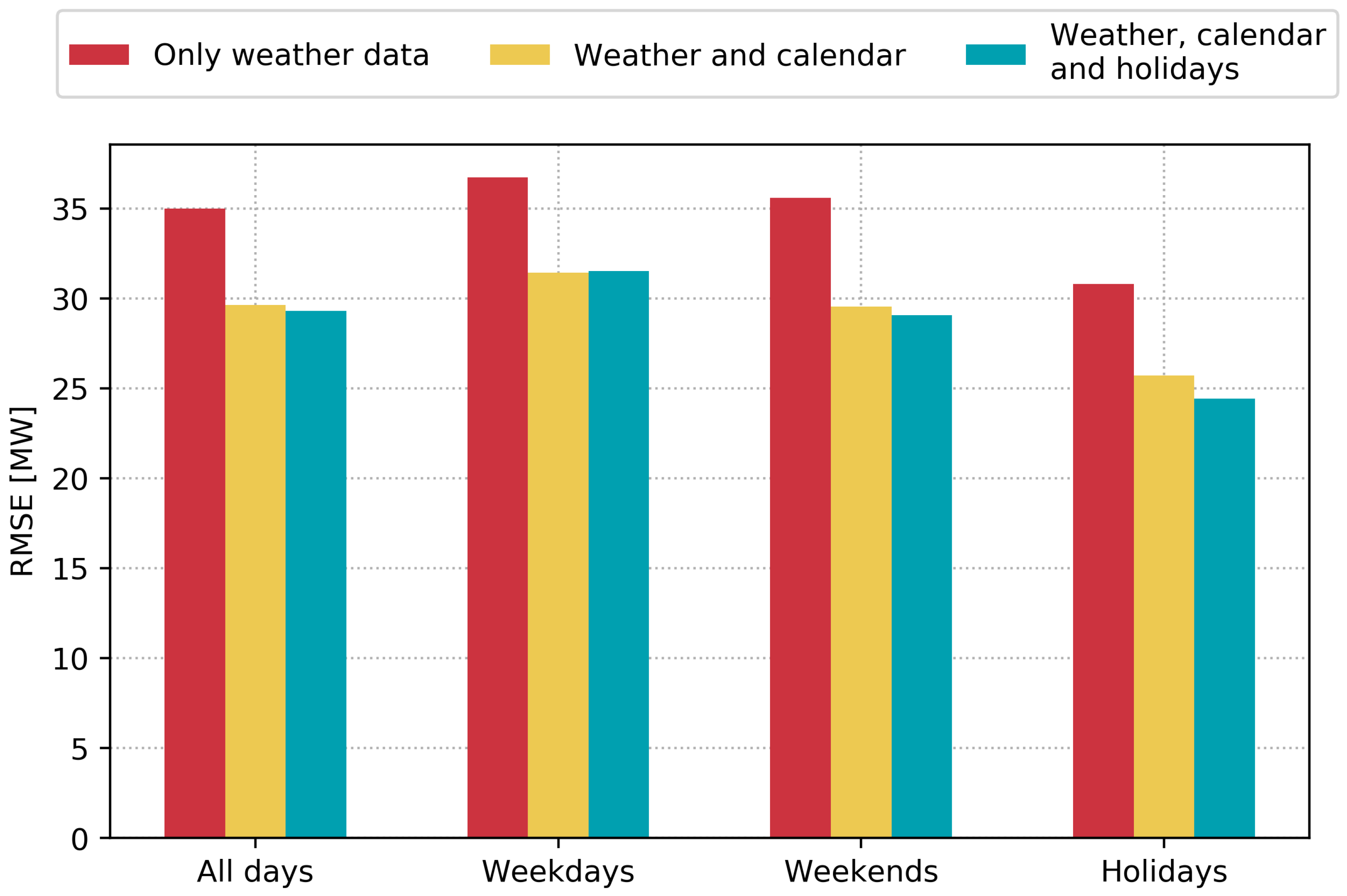
The goal of this analysis is to gauge the potential of including local holiday data in heat load forecasts in order to better capture the consumer behavior. The reduction in the annual error was very small when comparing models with only generic calendar data to models including local holiday data. This was clear from Figure 4b. It is well known among district heating operators that heat load forecasts tend to perform poorly on special occasions, such as Christmas or New Year’s Eve. These special days are rare, so the performance on those specific days has little impact on the average annual performance (Figure 4b). Improved performance on special days is valuable to production planners, and whether including local holiday data can improve forecast performance on specific days is worth investigating in more detail.
Figure 7 shows the performance of the SVR model in the three data scenarios on different sets of days during the year. “Holidays” refer to all days that are observances, national holidays, or school holidays. “Weekdays” include all weekdays that are not also in holidays, and “weekends” include all weekend days not included in holidays. In 2016, there were 201 weekdays, 65 weekend days, and 100 holidays.
There is significant benefit in including generic calendar data in the forecast models for all day types. On weekdays, there is no performance improvement to gain by including local holiday data. The forecast error on weekends can be reduced by 0.5 MW. Not surprisingly, the greatest performance increase can be observed on holidays. The holiday error decreases by 1.3 MW when augmenting the modeling with local holiday data. The holiday error is generally smaller than the error for the other day types. This is due to the holidays being dominated by the schools’ summer holidays, and the error is generally smaller during the summer. Summing up, including local holiday data only improves the forecasts slightly on average. The largest improvement is seen on holidays where the error can be reduced by 5%, compared to only using generic calendar data.
4. Conclusions
We have tested heat load forecasts with horizons from 15 h to 38 h, relevant for district heating production planning considering the day-ahead electricity market. The work was based on seven years of heat load and weather data for the large district heating system of Aarhus, Denmark. In order to measure the forecast performance that can realistically be experienced in actual operation, we used blind testing on a whole year with real weather forecasts.
Three machine learning models have been tested: an ordinary least squares model, a multilayer perceptron, and a support vector regression model. The SVR model performed best, beating the OLS model by a large margin and the MLP model by a small margin. All the models were trained on lagged heat load data and weather data. The forecast performance could be significantly improved by including generic calendar data, such as month, weekday, and hour of day. A smaller improvement of the forecasts could be gained by supplying the models with local holiday data including observances, national holidays, and school holidays. This improvement was most significant on holidays and weekends. Local holiday data can be difficult and time-consuming to obtain, but merely including lagged heat load, weather, and generic calendar data can provide a good overall forecast performance.
The SVR model using weather, calendar, and holiday data had the best performance. The root mean square error was 29.3 MW, and the mean absolute percentage error was 6.4%. This forecast model beat all other models that we have seen for the Aarhus system. The commercial forecast system, currently in operation in the Aarhus district heating system, had an RMSE of 41.9 MW, and a MAPE of 8.3% on the test year.
Including local holiday data showed only minor overall improvements in forecast performance, and including new data types in forecast models requires a careful evaluation of the trade-off between forecast accuracy and reliability of the data source. In live operational forecast systems, reliability is valued highly, and inputting data into a simpler model may work to make a more robust system. More features are thus not always an advantage, if the improvement in accuracy is insufficient to justify the added implementation and maintenance cost.
Initial experiments using long short-term memory networks have not shown notable improvement over the results attainable with the SVR model. However, future works should explore this type of model further, as it has the potential to simplify the feature selection procedure and make it easier to transfer these results to a wide range of district heating systems around the world.
Author Contributions
Conceptualization, G.B.A. and M.D.; Methodology, G.B.A. and M.D.; Formal Analysis, M.D.; Investigation, M.D. and O.S.K.; Data Curation, M.D.; Writing—Original Draft Preparation, M.D.; Writing—Review & Editing, G.B.A. and M.D.; Visualization, M.D.; Supervision, G.B.A. and A.B.; Project Administration, A.B.; Funding Acquisition, G.B.A. and A.B.
Funding
This research has received funding from the European Union’s Seventh Framework Programme for research, technological development and demonstration under grant agreement no ENER/FP7/609127/READY.
Acknowledgments
We would like to thank the Danish Meteorological Institute for providing the weather forecast data. We also thank AffaldVarme Aarhus for providing data about the heat load and production system in Aarhus.
Conflicts of Interest
The authors declare no conflict of interest.
Abbreviations
The following abbreviations are used in this manuscript:
| Heat load in hour t (MW) | |
| Heat load lagged by l hours (MW) | |
| Outdoor temperature in hour t (°C) | |
| Wind speed in hour t (m/s) | |
| Solar irradiation in hour t (W/m2) | |
| Outdoor temperature lagged by l hours (°C) | |
| Solar irradiation lagged by l hours (W/m2) | |
| Heat load forecasted for hour t (MW) | |
| L2 regularization parameter of the MLP model | |
| C | Regularization parameter of the SVR model |
| RBF kernel parameter of the SVR model | |
| RMSE | Root mean square error (MW) |
| MAE | Mean absolute error (MW) |
| MAPE | Mean absolute percentage error (%) |
| ME | Mean error (MW) |
| OLS | Ordinary least squares regression model |
| MLP | Multilayer perceptron model |
| SVR | Support vector regression model |
| RBF | Radial basis function kernel |
| LSTM | Long short-term memory network model |
References
- Ma, W.; Fang, S.; Liu, G.; Zhou, R. Modeling of district load forecasting for distributed energy system. Appl. Energy 2017, 204, 181–205. [Google Scholar] [CrossRef]
- Frederiksen, S.; Werner, S. District Heating and Cooling; Studentlitteratur: Lund, Sweden, 2013. [Google Scholar]
- Dotzauer, E. Simple model for prediction of loads in district-heating systems. Appl. Energy 2002, 73, 277–284. [Google Scholar] [CrossRef]
- Fang, T.; Lahdelma, R. Evaluation of a multiple linear regression model and SARIMA model in forecasting heat demand for district heating system. Appl. Energy 2016, 179, 544–552. [Google Scholar] [CrossRef]
- Grosswindhager, S.; Voigt, A.; Kozek, M. Online Short-Term Forecast of System Heat Load in District Heating Networks. In Proceedings of the 31st International Symposium on forecasting, Prague, Czech Republic, 26–29 June 2011. [Google Scholar]
- Nielsen, H.A.; Madsen, H. Modelling the heat consumption in district heating systems using a grey-box approach. Energy Build. 2006, 38, 63–71. [Google Scholar] [CrossRef] [Green Version]
- Idowu, S.; Saguna, S.; Åhlund, C.; Schelén, O. Forecasting heat load for smart district heating systems: A machine learning approach. In Proceedings of the 2014 IEEE International Conference on Smart Grid Communications (SmartGridComm), Venice, Italy, 3–6 November 2014. [Google Scholar]
- Izadyar, N.; Ghadamian, H.; Ong, H.C.; Moghadam, Z.; Tong, C.W.; Shamshirband, S. Appraisal of the support vector machine to forecast residential heating demand for the District Heating System based on the monthly overall natural gas consumption. Energy 2015, 93, 1558–1567. [Google Scholar] [CrossRef]
- Kusiak, A.; Li, M.; Zhang, Z. A data-driven approach for steam load prediction in buildings. Appl. Energy 2010, 87, 925–933. [Google Scholar] [CrossRef]
- Powell, K.M.; Sriprasad, A.; Cole, W.J.; Edgar, T.F. Heating, cooling, and electrical load forecasting for a large-scale district energy system. Energy 2014, 74, 877–885. [Google Scholar] [CrossRef]
- Kato, K.; Sakawa, M.; Ishimaru, K.; Ushiro, S.; Shibano, T. Heat load prediction through recurrent neural network in district heating and cooling systems. In Proceedings of the 2008 IEEE International Conference on Systems, Man and Cybernetics, Singapore, 15–16 May 2008; pp. 1401–1406. [Google Scholar]
- Nielsen, T.S.; Madsen, H. Control of Supply Temperature in District Heating Systems. In Proceedings of the 8th International Symposium on District Heating and Cooling, Trondheim, Norway, 14–16 August 2002. [Google Scholar]
- Hernández, L.; Baladrón, C.; Aguiar, J.M.; Calavia, L.; Carro, B.; Sánchez-Esguevillas, A.; García, P.; Lloret, J. Experimental analysis of the input variables’ relevance to forecast next day’s aggregated electric demand using neural networks. Energies 2013, 6, 2927–2948. [Google Scholar] [CrossRef]
- Saha, S.; Moorthi, S.; Pan, H.L.; Wu, X.; Wang, J.; Nadiga, S.; Tripp, P.; Kistler, R.; Woollen, J.; Behringer, D.; et al. The NCEP Climate Forecast System Reanalysis. Bull. Am. Meteorol. Soc. 2010, 91, 1015–1057. [Google Scholar] [CrossRef]
- Unden, P.; Rontu, L.; Järvinen, H.; Lynch, P.; Calvo, J.; Cats, G.; Cuxart, J.; Eerola, K.; Fortelius, C.; Garcia-Moya, J.A.; et al. HIRLAM-5 Scientific Documentation; Technical Report; Swedish Meteorological and Hydrological Institute: Norrkoping, Sweden, 2002. [Google Scholar]
- Holidays in Denmark. Available online: www.timeanddate.com/holidays/denmark/ (accessed on 13 June 2017).
- Crawley, D.B.; Hand, J.W.; Kummert, M.; Griffith, B.T. Contrasting the capabilities of building energy performance simulation programs. Build. Environ. 2008, 43, 661–673. [Google Scholar] [CrossRef] [Green Version]
- Dahl, M.; Brun, A.; Andresen, G.B. Decision rules for economic summer-shutdown of production units in large district heating systems. Appl. Energy 2017, 208C, 1128–1138. [Google Scholar] [CrossRef]
- Alpaydin, E. Introduction to Machine Learning; MIT Press: Cambridge, MA, USA, 2014. [Google Scholar]
- Bishop, C.M. Pattern Recognition and Machine Learning; Springer: New York, NY, USA, 2006. [Google Scholar]
- Hochreiter, S.; Schmidhuber, J. Long short-term memory. Neural Comput. 1997, 9, 1735–1780. [Google Scholar] [CrossRef] [PubMed]
- Drucker, H.; Burges, C.J.; Kaufman, L.; Smola, A.J.; Vapnik, V. Support vector regression machines. In Advances in Neural Information Processing Systems; MIT Press: Cambridge, MA, USA, 1997; pp. 155–161. [Google Scholar]
- Pedregosa, F.; Varoquaux, G.; Gramfort, A.; Michel, V.; Thirion, B.; Grisel, O.; Blondel, M.; Prettenhofer, P.; Weiss, R.; Dubourg, V.; et al. Scikit-learn: Machine learning in Python. J. Mach. Learn. Res. 2011, 12, 2825–2830. [Google Scholar]
- Dahl, M.; Brun, A.; Andresen, G.B. Using ensemble weather predictions in district heating operation and load forecasting. Appl. Energy 2017, 193, 455–465. [Google Scholar] [CrossRef]
- Scott, D.W. On optimal and data-based histograms. Biometrika 1979, 66, 605–610. [Google Scholar] [CrossRef]
Figure 1.
Timeline for the heat load forecast that is relevant for the trading decisions in the day-ahead electricity market. Every day at 10:00 a forecast is produced for each hour of the following day.
Figure 1.
Timeline for the heat load forecast that is relevant for the trading decisions in the day-ahead electricity market. Every day at 10:00 a forecast is produced for each hour of the following day.

Figure 2.
Time series for the hourly heat load in the year 2010. The inset shows a zoom of a week in March.
Figure 2.
Time series for the hourly heat load in the year 2010. The inset shows a zoom of a week in March.

Figure 3.
Example forecasts for 4 May 2016. The forecasts were produced on 3 May at 10:00 and based on real weather forecasts, calendar, and holiday data.
Figure 3.
Example forecasts for 4 May 2016. The forecasts were produced on 3 May at 10:00 and based on real weather forecasts, calendar, and holiday data.

Figure 4.
Root mean square error of the three forecast models OLS, MLP, and SVR on the year 2016. The top panel (a) shows the error using historical weather data to simulate 100% accurate weather forecasts. The bottom panel (b) shows the error using real weather forecasts.
Figure 4.
Root mean square error of the three forecast models OLS, MLP, and SVR on the year 2016. The top panel (a) shows the error using historical weather data to simulate 100% accurate weather forecasts. The bottom panel (b) shows the error using real weather forecasts.

Figure 5.
Performance of the SVR model on the year 2016, using real weather forecasts, calendar, and holiday data. Three different error metrics are shown for each month of the year. The forecast error varies with the time of day, shown on the horizontal axes. RMSE (blue) and MAE (yellow) are shown units of MW on the left axes. MAPE (red) is shown in percent on the right axes.

Figure 6.
Histograms for the forecast error of the SVR model on the year 2016 using real weather forecasts, calendar, and holiday data. The distribution of the forecast error is depicted for each month in the year along with the 10% and 90% quantiles. The number of bins was chosen using Scott’s rule [25] within each month. A positive error indicates that the forecast was too high, a negative error that it was too low.

Figure 7.
Forecast performance of the SVR model on the year 2016 using real weather forecasts, calendar, and holiday data. The second and third group of bins refer to weekdays and weekends that are not also included in holidays. Holidays refer to all days that are observances, national holidays, or school holidays (see Table 1).


Table 1.
Input variables used in the three data scenarios (in bold).
| Only Weather Data | Weather and Calendar | Weather, Calendar and Holidays | ||
|---|---|---|---|---|
| Lagged heat load | or | ✓ | ✓ | ✓ |
| ✓ | ✓ | ✓ | ||
| Weather data | ✓ | ✓ | ✓ | |
| ✓ | ✓ | ✓ | ||
| ✓ | ✓ | ✓ | ||
| ✓ | ✓ | ✓ | ||
| ✓ | ✓ | ✓ | ||
| Calendar data | Hour of day | ✓ | ✓ | |
| Day of week | ✓ | ✓ | ||
| Weekend | ✓ | ✓ | ||
| Month of year | ✓ | ✓ | ||
| Holiday data | National holiday | ✓ | ||
| Observance | ✓ | |||
| School holiday | ✓ |
Table 2.
Summary of the hourly forecast error for each month for the SVR model using real weather forecasts, calendar, and holiday data. Histograms of the forecast error appear in Figure 6. The months with the worst performance are indicated in red, the best in green. The quantiles are evaluated in pairs, so the widest symmetric quantile interval is considered the worst.
| RMSE | ME | Error Quantiles (MW) | ||||
|---|---|---|---|---|---|---|
| (MW) | (MW) | 10% | 90% | 1% | 99% | |
| January | 41.2 | 18.7 | −24.0 | 64.1 | −66.8 | 117.6 |
| February | 31.8 | −2.2 | −42.8 | 36.6 | −91.6 | 61.3 |
| March | 36.9 | 2.0 | −43.7 | 48.8 | −80.4 | 89.3 |
| April | 34.2 | −11.7 | −52.9 | 27.1 | −93.6 | 64.8 |
| May | 18.2 | 4.3 | −14.7 | 25.6 | −33.6 | 64.3 |
| June | 15.8 | −3.3 | −19.3 | 12.8 | −45.3 | 34.0 |
| July | 10.6 | 5.0 | −7.0 | 17.2 | −16.0 | 25.8 |
| August | 14.2 | 6.9 | −8.2 | 21.6 | −20.1 | 41.6 |
| September | 14.3 | 0.3 | −17.9 | 17.6 | −35.0 | 33.3 |
| October | 25.6 | 4.8 | −26.0 | 37.8 | −43.5 | 70.0 |
| November | 38.1 | 20.5 | −20.0 | 61.5 | −59.1 | 98.1 |
| December | 43.1 | 12.5 | −38.4 | 58.2 | −96.7 | 115.0 |
© 2018 by the authors. Licensee MDPI, Basel, Switzerland. This article is an open access article distributed under the terms and conditions of the Creative Commons Attribution (CC BY) license (http://creativecommons.org/licenses/by/4.0/).
Share and Cite
MDPI and ACS Style
Dahl, M.; Brun, A.; Kirsebom, O.S.; Andresen, G.B. Improving Short-Term Heat Load Forecasts with Calendar and Holiday Data. Energies 2018, 11, 1678. https://doi.org/10.3390/en11071678
AMA Style
Dahl M, Brun A, Kirsebom OS, Andresen GB. Improving Short-Term Heat Load Forecasts with Calendar and Holiday Data. Energies. 2018; 11(7):1678. https://doi.org/10.3390/en11071678
Chicago/Turabian StyleDahl, Magnus, Adam Brun, Oliver S. Kirsebom, and Gorm B. Andresen. 2018. "Improving Short-Term Heat Load Forecasts with Calendar and Holiday Data" Energies 11, no. 7: 1678. https://doi.org/10.3390/en11071678
Note that from the first issue of 2016, this journal uses article numbers instead of page numbers. See further details here.