Historical Evolution of the Wave Resource and Energy Production off the Chilean Coast over the 20th Century

Abstract

The wave energy resource in the Chilean coast shows particularly profitable characteristics for wave energy production, with relatively high mean wave power and low inter-annual resource variability. This combination is as interesting as unusual, since high energetic locations are usually also highly variable, such as the west coast of Ireland. Long-term wave resource variations are also an important aspect when designing wave energy converters (WECs), which are often neglected in resource assessment. The present paper studies the long-term resource variability of the Chilean coast, dividing the 20th century into five do-decades and analysing the variations between the different do-decades. To that end, the ERA20C reanalysis of the European Centre for Medium-Range Weather Forecasts is calibrated versus the ERA-Interim reanalysis and validated against buoy measurements collected in different points of the Chilean coast. Historical resource variations off the Chilean coast are compared to resource variations off the west coast in Ireland, showing a significantly more consistent wave resource. In addition, the impact of historical wave resource variations on a realistic WEC, similar to the Corpower device, is studied, comparing the results to those obtained off the west coast of Ireland. The annual power production off the Chilean coast is demonstrated to be remarkably more regular over the 20th century, with variations of just 1% between the different do-decades.

1. Introduction

Ocean waves store a tremendous potential that is still untapped. The main reason why wave energy has not been yet exploited is the difficulty to economically harvest energy from ocean waves. Different technological solutions have been suggested in recent decades [1], but none of these technologies has achieved yet economical viability to compete in the energy market with other more established energy sources. The Mutriku wave energy plant, based on the oscillating water column principle, is one of the examples of wave energy converters (WECs), which is the first wave energy plant connected to the electricity grid. Despite its aim to be an experimental plant, the plant has achieved a capacity factor (CF) of 11% in the first years of operation [2], showing WECs can be an additional alternative to reduce greenhouse emissions.

In the way towards designing technically and economically viable WECs, there are several aspects to be improved, such as the survivability of the devices, the cost reduction in the construction stage, minimisation of maintenance operations, energy maximisation via control strategies and design of efficient power take-off (PTO) systems. A precise assessment of the wave energy resource is also essential to accurately design WECs and maximise the power extraction from ocean waves. Wave energy converters, based on different working principles and deployed in different locations, are analysed in [3], where the CF of each WEC varies significantly depending on the wave climate in each location.

In particular, the variability of the resource, both inter- and intra-annual variability, is a critical aspect that can affect the design of the WEC. Intra-annual variations of the resource have been analysed in different spatial scales [4,5,6]. However, historical long-term variations of the wave climate have been often neglected. The authors have studied these long-term variations in the Bay of Biscay and off the west coast of Ireland in [7] and [8], respectively, analysing wave trends over the 20th century and the influence of these trends in the performance of specific WECs. In both locations, positive trends have been found, with wave height ($H_s$), peak period ($T_p$) and wave energy flux ($WEF$) increasing significantly over the 20th century.

The evaluation of the wave energy potential in a specific location usually involves a combination of observations (buoys and satellites), reanalyses and, sometimes, numerical modelling with models such as SWAN or Mike 21. Using these techniques, several studies have recently focused on different parts of the American continent for wave energy potential assessment [9,10,11]. The Chilean coast is one of the interesting areas in South America for the implementation of WEC farms, with an estimated resource of about 165 GW along its 5000 km [12]. This background has encouraged researchers to study the potential of specific converters at specific locations [13].

Chile and the west coast of Ireland are considered paradigmatic examples, with respect to their wave energy resource. Both present high mean wave power, but the wave resource off the west coast of Ireland is highly variable, while the resource off the Chilean coast is more consistent. This contrast is shown in [14], based on measurements collected by several buoys around the world, via the coefficient of variation ($COV$), which is given as follows,

$$COV=\frac{\sigma \left(WEF\right)}{\overline{WEF}},$$

(1)

where $\sigma \left(WEF\right)$ is the standard deviation (SD) of the $WEF$ and $\overline{WEF}$ is the average of the $WEF$.

Ringwood and Brandle [14] showed that the maximum $COV$ for Chile is 0.9, which is observed in the south of the Chilean coast, where the $WEF$ is about 121 kW/m. In contrast, the $COV$ for Ireland is 1.8 (twice as high as the maximum $COV$ for Chile), where the mean wave power is lower than for the southern Chilean coast: 95 kW/m. Therefore, Chile shows a high energetic and consistent wave resource, which is important in the process to harness and produce energy from ocean waves.

The most recent validation of wave energy assessment in Chile covers the 1989–2013 period [15], where a third generation wave model is used, validated against buoy measurements, to generate three-hourly sea-state parameters ($H_s$-$T_p$ pairs). These data are then propagated from offshore to nearshore locations by means of the SWAM model, to characterise the wave climate along the entire coast. Validation results show good agreement between modelled and measured data, with errors of less than 10%. Wave power and seasonal variability in Chile increase with the latitude, which fluctuates between 20 and 35 kW/m in the areas close to shore, and where the most energetic sea-states happen in winter. These results and others [16] show lower wave resource potential, about 5–10 kW/m lower, compared to previous studies, which suggests that previous assessments may have overestimated the wave resource [17].

However, these studies have been developed within a period of 30–40 years, and, thus, historical trends of wave energy are not considered. In the present study, the objective was to analyse the long-term variability of the wave energy resource in Chile, studying the wave energy resource in Chile over the 20th century and comparing the results from the Chilean coast to other locations. Following the recommendations by the World Meteorological Organization [18,19], reliable estimation of climate variables requires at least 30 years of data. These data may be obtained by means of different techniques: buoy measurements [20], observations from ships [21,22], satellite altimeter [23,24] or models and reanalysis datasets [5,25,26,27,28,29,30,31]. The latter method was used in the present study, using the ERA20 reanalysis from the European Centre for Medium-Range Weather Forecasts (ECMWF), calibrated with the ERA-Interim (ERAI) reanalysis.

Among the different techniques to estimate climate variables, the satellite altimeter has considerably improved in the recent decades, generating very interesting data for long-term wind or wave trends. For instance, Young et al. [24] presented a study of wind speed and wave height trends in a global scale, which is the only study, to the best of authors’ knowledge, that covers the same area of study analysed in the present paper (the Chilean shoreline). However, the time period analysed in [24] is shorter, 23 years between 1985 and 2008, and only the trends of wave heights are analysed, which may be insufficient to draw strong conclusions on the historical wave energy trends, since the influence of the wave period is demonstrated to be essential [7]. Young et al. [24] showed a significant statistical trend for wave heights, analysing mean monthly values in the east of Africa, in the east of North America and the west of South America (the Chilean coast and south-eastern Pacific Ocean). Furthermore, the increase of wind speed is very important in Chile, due to the effect of a hot spot (a positive trend of 15%/decade) in the middle of the Pacific Ocean at equatorial latitudes. Thus, according to [24], wave height trends are large in Chile, showing a positive trend between 0% and 0.25% per year, meaning that a typical wave of 2 m height would increase about 5 cm per decade.

A similar analysis is carried out in [30,31], where the global wave energy resource is assessed via the ERA40 reanalysis, the previous version of the ERAI reanalysis used in this paper. Wave trends in [30,31] are calculated by means of a linear regression. As for the study carried out in [24], positive wave trends are found in [30,31] for the Chilean coast, where these trends are also shown to increase with the latitude. More precisely, wave trends of about 1 kW/m/decade are found in the north of the Chilean coast, while trends of 2 kW/m/decade are observed in the south, which implies about 3.3%/decade for a mean wave power of 60kW/m. Additionally, other studies, such as [32], also show long-term wave energy resource variations in several areas.

Therefore, a precise characterisation of the resource requires the analysis of long-term variations, including a time-evolving description of the resource, to accurately understand the resource in which the WEC is deployed. However, wave energy resource assessment studies commonly rely on recent past data (typically, between 10 and 30 years of past data), and analyse the resource as a static element, even though it has been widely demonstrated that the ocean is a highly dynamic environment [7,14,30,31]. The objective of this paper is to fill this gap for the Chilean coast, analysing the long-term trends of wave energy over the 20th century. In addition, the impact of these variations is evaluated on a realistic point absorber (PA) type WEC, similar to the real Corpower device.

The remainder of the paper is as follows: Section 2 presents the datasets and the methodology to calibrate and study the wave trend, Section 3 describes the realistic WEC and the hydrodynamic model employed to evaluate its power absorption, Section 4 shows the results related to the resource variations and the power absorptions, Section 5 discusses the results and Section 6 presents the conclusions of the study.

2. Wave Data and Methodology

2.1. Wave Data

Two different sources of wave data are used in this paper. On the one hand, two reanalyses of the ECMWF are employed and, on the other hand, wave data collected via buoy measurements is used. Further information about both ECMWF reanalyses and buoy measurements is given in Section 2.1.1 and Section 2.1.2.

2.1.1. ERA20C and ERA-Interim Reanalyses

The two reanalyses of the ECMWF used in this study are the ERA20C and ERA-Interim reanalyses (ERA20 and ERAI henceforth). The ERA20 reanalysis is ECMWF’s first atmospheric reanalysis, which covers the whole 20th century. In the ERA20 reanalysis, observations of surface pressure and surface marine winds are assimilated [33] by means of a 4D-Var analysis. More observations are available, the more reliable are the data generated via the ERA20 reanalysis [34]. Consequently, the data provided by the ERA20 reanalysis are more accurate in the northern hemisphere, although they have also been used for the study of historical wave trends and coastal evolution in different locations of the southern hemisphere [35,36,37]. The spatial resolution of the ERA20 reanalysis is approximately 125 km and wave parameters can be obtained three-hourly [34].

The ERAI reanalysis is also a global reanalysis, but only covers the time period since 1979. The wave model implemented in the ERAI reanalysis is the Wave Modelling Project (WAM) approach [38], which reduces the error in the wave period assimilation, compared to previous ECMWF reanalyses, such as the ERA40 [39]. The ERAI reanalysis also assimilates data via a 4D-Var method, but using a 75 km spatial resolution and providing wave parameters every six hours [40].

Therefore, the ERA20 reanalysis was calibrated against the ERAI reanalysis, providing more precise wave data for the whole 20th century. Due to the discrepancy of the temporal resolution between ERA20 and ERAI, only six-hourly data were used in the calibration and the calibration was carried out in the intersection period between both reanalyses, which spans 32 years from 1979 to 2010.

2.1.2. Buoy Measurements

Buoy data used in the present study were provided by the SHOA (Spanish acronym of the Chilean Navy Hydrographic and Oceanographic Service). Data from two specific locations were used, i.e., Iquique and Valparaiso, depicted in Figure 1 together with the complete study area, from the Magellan Strait to the Peruvian border in the southern Pacific Ocean.

Table 1. Main characteristics of the buoys.

Buoy	Longtitude	Latitude	Distance (km)	Period
Iquique	−70.25	− 20.25	38	2004–2008
Valparaiso	−71.65	−32.97	33	2000–2003

shows the characteristics of the two buoys: the exact position (longitude, latitude), the distance to the nearest gridpoint in the reanalyses and the time period in which data were collected.

2.2. Methodology

2.2.1. Computation of the Wave Energy Flux

Although the $WEF$ is directly obtained from the parameters available in the reanalysis, it can be given as a function of $H_s$ and the energy period ($T_e$) as follows [41],

$$WEF=0.49H_s^2{T}_e.$$

(2)

However, the wave period data provided by SHOA include only $T_p$ for our validation. Therefore, to calculate the $WEF$ at the buoy, Equation (2) needs to be adapted by including a correction coefficient between $T_e$ and $T_p$, similar to the $\alpha =T_e/T_p$ coefficient described in [42]. According to this study, for a standard JONSWAP spectrum, $\alpha$ reaches 0.90. We took into account the correction factor $\alpha$ for $T_p$ given by the reanalysis data in the validation procedure at the buoy’s nearest gridpoint. The power matrix of the WECs is given also for $T_p$ and this period was therefore used for the analysis of the production of our device.

On the other hand, Wave Period Ratio (WPR) described in [7,8,41] which relates the energy period to the average zero-crossing period was obtained for the trend computation of wave period. The WPR changes depending on the area of study, which, in the case of Iquique and Valparaiso, lies between 0.8 and 1. Furthermore, mean wave period and average zero-crossing period are very similar, within an error of 10% for monthly means values used for the trends. In any case, this kind of scale factors does not affect the results of the trends, since they constitute the relative slopes of the absolute values. Thus, $T_m$ is the chosen period for the representation of maps, because it is one of the most frequently used parameters for the description of the wave period.

2.2.2. Directional Quantile-Matching Calibration

The calibration or bias correction is usually referred to as the classified quantile-matching method, although it has also been named in the literature as probability mapping [43], quantile-quantile mapping [44,45], statistical downscaling [46] or histogram equalization [47]. This calibration method is commonly used in the literature to calibrate temperature, precipitation, wind speed or other parameters [48,49,50,51,52].

The classified quantile-matching method presented in this paper allows for a more sophisticated classified calibration, where the relevance of each variable in the calibration can be considered. Hence, instead of using a single transfer function for the whole time-series, as in the previous studies of the authors [7,8], different transfer functions are used for each time-interval. In the case of wind speed, the variable used for the classification can be directionality, using four main wind directions (northeast, southeast, northwest and southwest). That way, a different transfer function is obtained for each direction interval, for a total of four transfer functions.

Another option is selecting irregular directional intervals to match the specific characteristics, i.e. the predominant wind directions, of the location under analysis. This type of classification is known as wind rose bias correction [53], which is an interesting approach for wave resources, due to their directional characterisation. The closer to the shore, the more defined this directionality is, which in the case of the Chilean coast, is significantly dominated by the western waves. More specifically, the predominant wave direction in Iquique and Valparaiso, illustrated by the wave roses depicted in Figure 2, is the southwest direction. Therefore, the strong directionality of the wave resource in Iquique and Valparaiso justifies the use of the classified quantile-matching technique for the calibration, using wave direction as the variable for the classification.

To consider the directionality of the wave resources, seven transfer functions for seven intervals of wave direction, following the wave roses in Figure 2, have been created. Hence, the northeast, southeast and northwest quadrants are represented by a single interval of 90${}^{\circ }$, while the southeast quadrant is divided into four different intervals of 22.5${}^{\circ }$. Although the comparative of different types of distributions is out of the scope of this paper, the seven-interval distribution has been compared via proof and error to other distribution schemes, such as four quadrant or eight octant regular distributions, where the seven-interval distribution scheme provides the best results. In any case, the visual intuition provided by the wind roses is enough to justify the decision.

In previous studies by the authors in the Bay of Biscay and west coast of Ireland [7,8], no classification technique is used in the calibration, and, consequently, this directionally-classified quantile-matching technique can be considered as a novel contribution of this paper in the context of wave energy. To the best of authors’ knowledge, this is the first time that a wave rose bias correction is used, analogous to the aforementioned “wind rose bias correction”.

This method is a statistical method that matches the values with the same quantile between the ERA20 and ERAI reanalyses. Hence, by calibrating the ERAI reanalysis against the ERA20 reanalysis, using the directionally-classified quantile-matching technique, directionally-calibrated wave data (dcERA20) can be obtained. The process is divided into the following steps:

• Classify sea events according to the previously selected direction intervals.
• Compute the $WEF$ of each event for the ERAI and ERA20 reanalyses in their intersection period (1979–2010).
• Calculate the cumulative probability functions for both reanalyses.
• Obtain a transfer function between the couple of $WEF$ values with the same quantile, for each direction interval in the intersection period.
• Apply these transfer functions to all the historical values of ERA20 (1900–2010) to obtain the calibrated dcERA20 time-series.
• Verify the calibrated values against buoy measurements collected at the closest point.

2.2.3. Evaluation Metrics

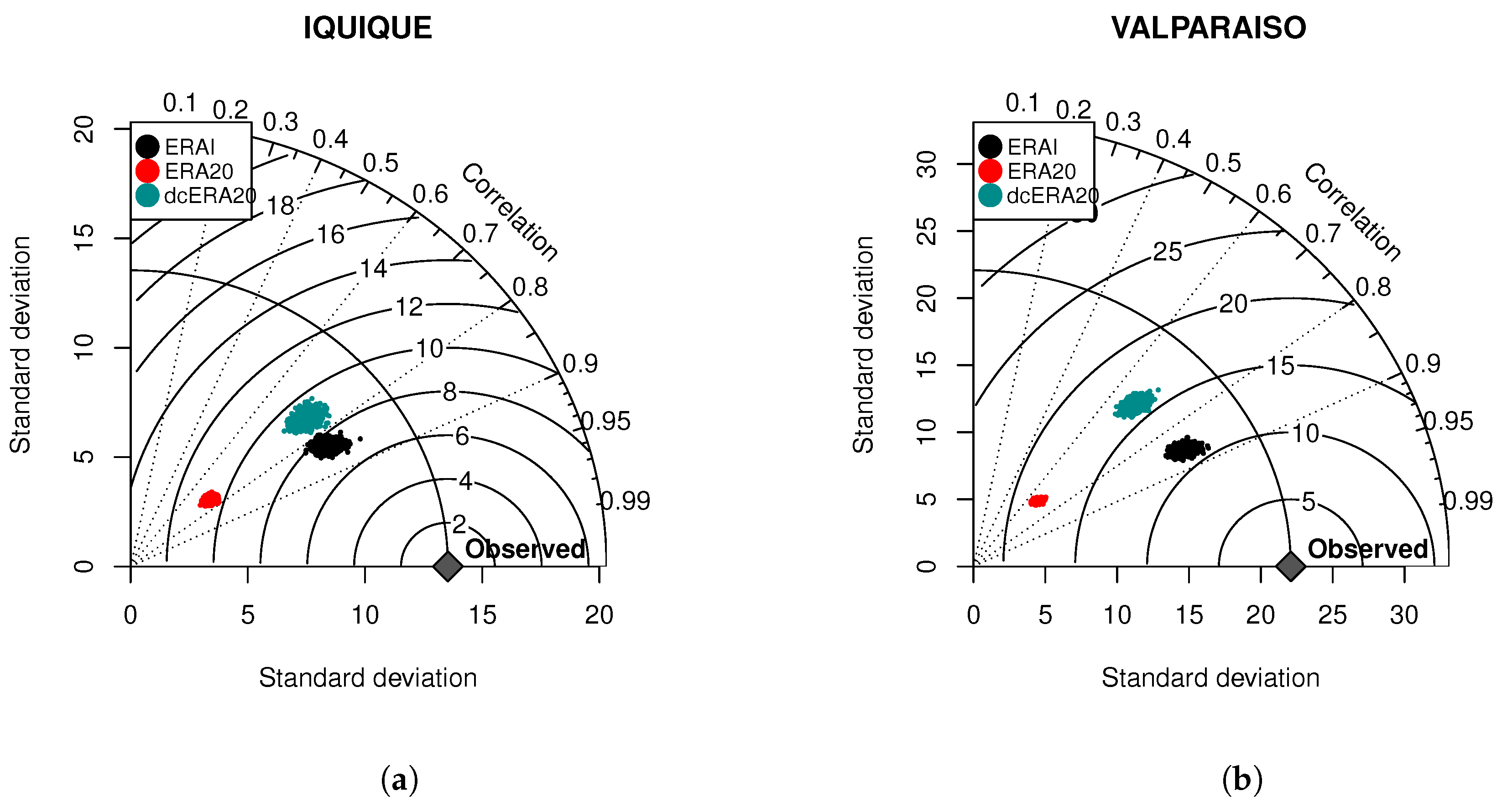
Six statistical metrics were used for the validation of the calibration procedure against the two buoys, that is to say, to compare the non-calibrated data from the ERA20 reanalysis with the directionally-calibrated dcERA20 wave data and the ERAI reanalysis, used as the basis of the calibration:

• Pearson’s correlation of the $WEF$, represented by the exterior arc of a Taylor Diagram [54].
• The root mean square error (RMSE) for the $WEF$, represented by the interior arc of a Taylor Diagram centred on the Observation point.
• The SD of the $WEF$ series represented by the interior arc of a Taylor Diagram that passes from the observation point on the X axis. This allowed for a visual comparison of the variability given by the SD in the observations and the wave models.
• The variability of the data in relative terms was also analysed by the previously mentioned $COV$.
• The bias of the $WEF$ with respect to the buoy measurements, which can be more relevant than the RMSE or other absolute errors, since it facilitates to identify under- and over-estimation.
• The mean absolute percentage error (MAPE) of the $WEF$, which represents the absolute error to be reduced by the calibration procedure.

2.2.4. Wave Resource Maps

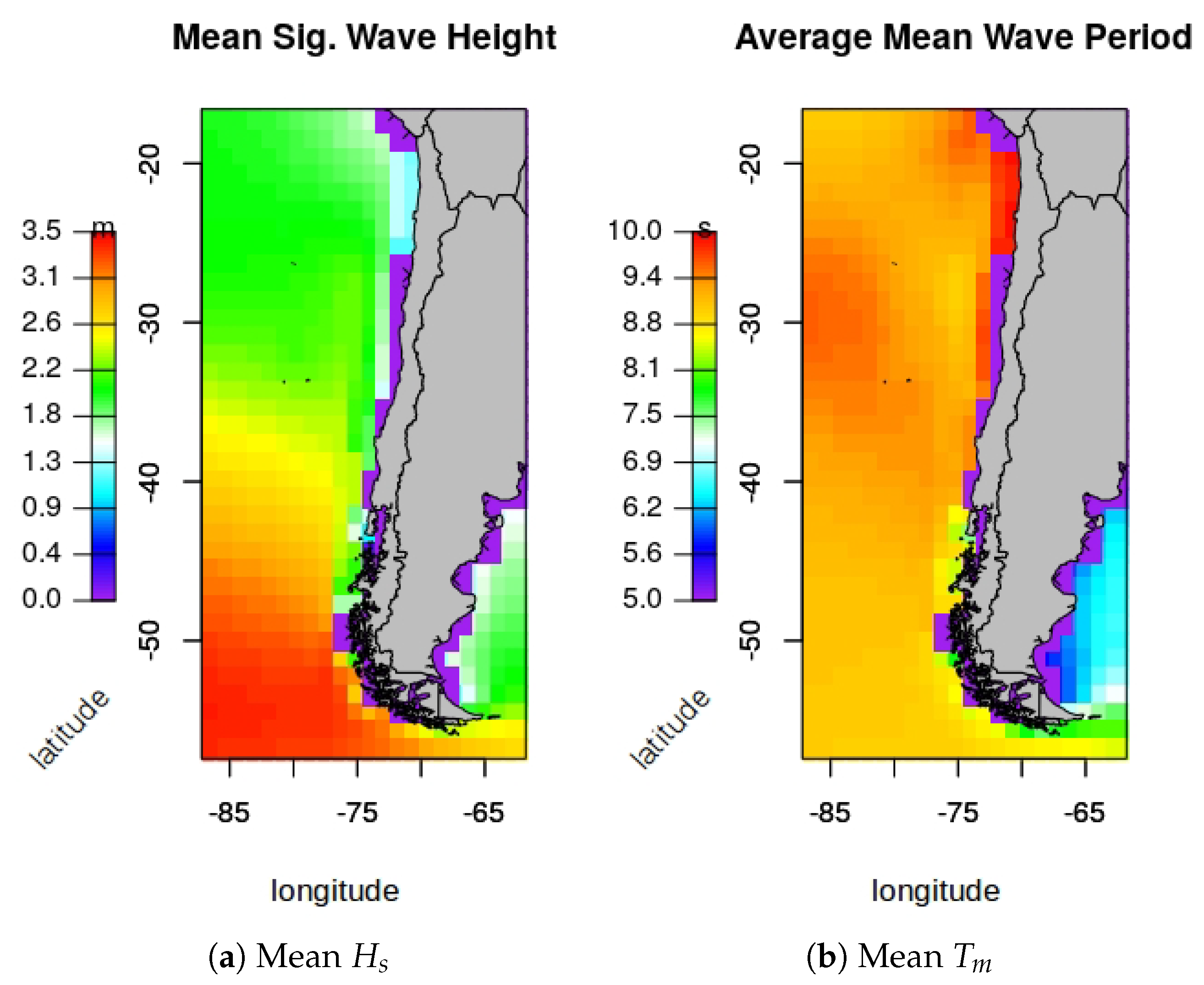
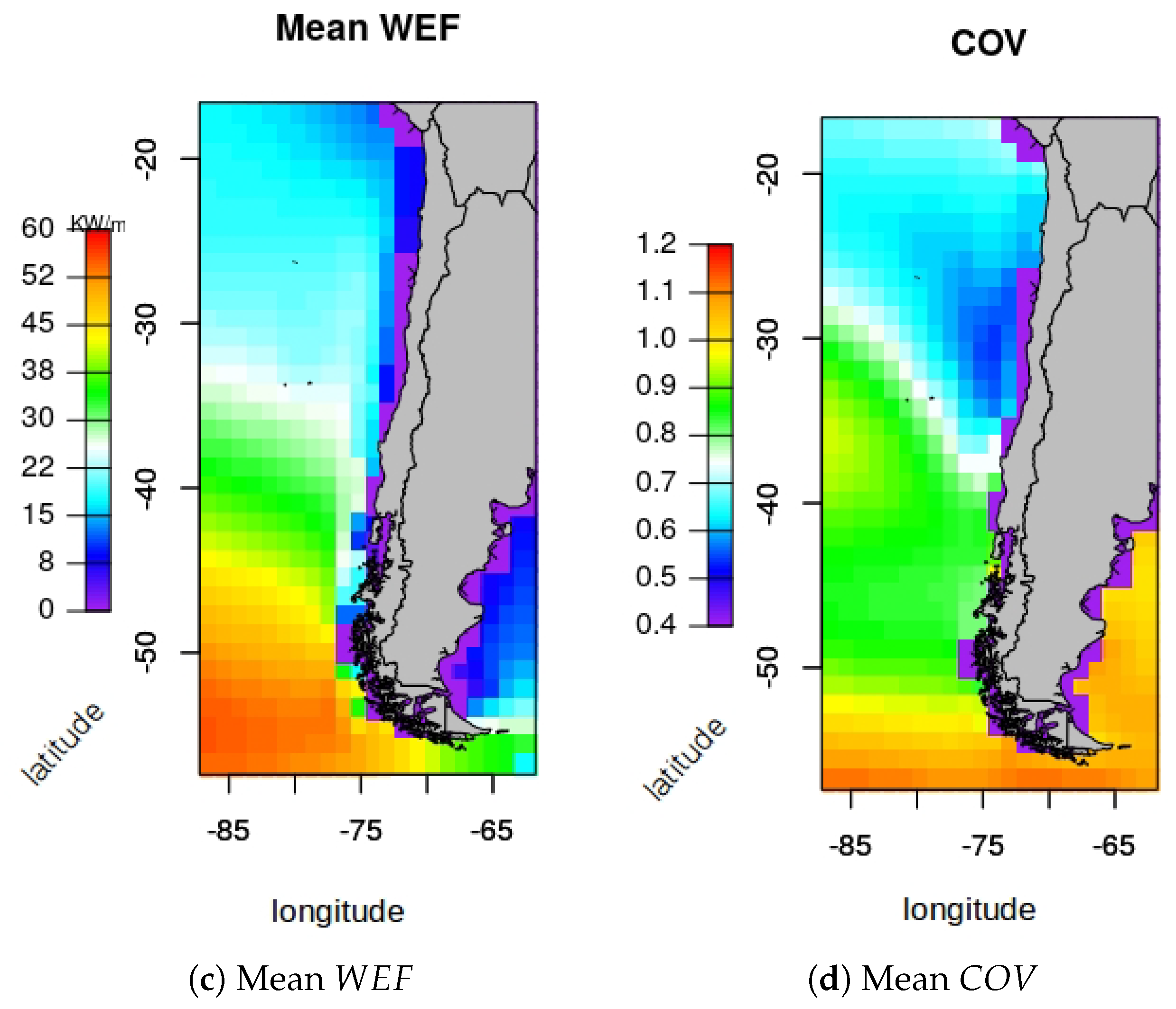
The historical evolution of the resource is also represented by means of maps, showing wave trends of the entire area of study. The trends were computed using the non-parametric Theil-Sen [55,56] method, which fits a line using the median of the slopes. The significance of the trend at each grid point was evaluated at a 95% confidence level using bootstrap resampling with 1000 samples.

Thus, different variables are illustrated using maps:

• The average $H_s$, $T_m$ and $WEF$ values for the entire area of study, based on the ERAI reanalysis, which provides a picture of the wave resource in the recent decades. In addition, the map with the average $WEF$ is useful to identify the highest energetic locations (see Section 4.2.1).
• The $COV$ over the whole study area, also based on the ERAI reanalysis. Together with the average $WEF$ map, the $COV$ map can help to identify interesting locations for the implementation of WEC farms (see Section 4.2.1).
• Decadal trends of the average $H_s$, $T_m$ and $WEF$ values over the 20th century, using the dcERA20 reanalysis, to show resource variations (Section 4.2.2).
• Decadal trends of the seasonal $WEF$ for the four seasons. The seasonal analysis provides more insight into the contribution of each season to the annual wave energy trend (Section 4.2.3).

3. Hydrodynamic Modelling

Several different WECs have been suggested in the literature to extract energy from ocean waves. Based on their working principles, all WEC can be categorised into four main groups [1]: overtopping devices, oscillating water column devices, oscillating wave surge converters and PAs. Although none of the prototypes suggested so far has yet achieved commercial viability, a large part of the most developed prototypes are PAs, such as the CETO [57], Seabased [58] and the Corpower [59] devices. The PA used in this study is inspired by the Corpower device, referred in the following as the cPA, illustrated in Figure 3a, adapted from [60]. Further details about the characteristics of the WEC implemented in this study are provided in [8].

Power production capabilities of the cPA for a wide range of sea-states, represented using irregular-wave time-series based on the JOSNWAP spectrum [61], were estimated via numerical simulation, computing the power-matrix depicted in Figure 3b. The behaviour of the cPA in this study was evaluated by analysing its motion in two degrees of freedom, as in [59], following the linear Cummins’ equation [62] as follows,

$$(M+{\mu }_{\infty })\ddot{x}\left(t\right)=F_{ex}-K_{H}x-{\int }_0^t{K}_{rad}(t-\tau )\dot{x}\left(\tau \right)dt+F_{visc}+F_{PTO}+F_{MOO}+F_{EndStop},$$

(3)

where M and ${\mu }_{\infty }$ are the mass and infinite added-mass matrices; x, $\dot{x}$ and $\ddot{x}$ are the displacement, velocity and acceleration of the device, respectively; $F_{ex}$ is the excitation force; $K_H$ is the hydrostatic stiffness; $K_{rad}$ is the radiation impulse response; $F_{PTO}$ is the PTO force; $F_{MOO}$ is the mooring force; and $F_{EndStop}$ is the force that reproduces the end-stop effect of the PTO mechanism. The only nonlinearity included in the model is the viscous force ($F_{visc}$), which is modelled using a quadratic damping based on a Morison-like equation [63] as follows,

$$F_{visc}=\frac{1}{2}\rho C_D{A}_D(\dot{x}-V_0)|\dot{x}-V_0|$$

(4)

where $\rho$ is the water density, $C_D$ is drag coefficient, $A_D$ is the characteristic area of the WEC and $V_0$ is the velocity of the undisturbed water flow.

The objective of the present study was to study the impact of wave energy resource variations, assessing the power produced by the cPA over the 20th century off the Chilean coast. Nonlinear effects, such as nonlinear Froude–Krylov forces, are shown to be essential for accurately estimating power production capabilities of PAs [64] and, more specifically, for the Corpower device [65]. However, since the authors are only interested in the relative values of the comparison, the mathematical model based on the linear Cummins’s equation is considered adequate.

Similarly, the need for including the most relevant PTO dynamics, losses and constraints to accurately estimate power production capabilities of a WEC is demonstrated in [66]. Nevertheless, the present paper focuses on the impact of wave energy resource variations, for which analysing power absorption is found sufficient. However, constraints of the PTO system significantly affect the power absorption of a WEC. Therefore, three main constraints usually included by any PTO system, i.e., displacement, velocity and force constraints, are also considered, similar to [67].

4. Results

4.1. Evaluation Versus Buoys

Figure 4a,b illustrates the Taylor Diagrams for the Iquique and Valparaiso locations, respectively, where Pearson’s correlation, the RMSE and the SD between the ERA20, ERAI and dcERA20 reanalyses are shown. The correlation of the dcERA20 reanalysis is shown to be very similar to that of the original ERA20, meaning that the correction did not improve the correlation. The correlation of the ERAI reanalysis, which is the upper limit for the calibration, is shown to be about 0.9 in both locations, while the ERA20 and dcERA20 show correlations of about 0.7–0.8. However, the dcERA20 reanalysis shows reasonable improvement in RMSE and SD. The RMSE for the ERA20 reanalysis is above 10 kW/m for Iquique, while reducing below that threshold after calibration. The RMSE reduction is even more significant for Valparaiso, reducing the $WEF$ from 20 kW/m to 15 kW/m. In the case of the SD ratio, which shows the ratio between SDs of the wave models and buoy measurements, the calibration corrects the SD from 4/14 to 11/14 in Iquique, and from 6/22 to 18/22 in Valparaiso, which mean an improvement of over 50% in both cases. Hence, despite the low impact of the calibration on the correlation, the calibration is shown to significantly improve the wave data, approaching the more reliable ERAI reanalysis.

Analysing other metrics described in Section 2.2.3, the effect of the calibration is even more evident, as shown in

Table 2. Mean $WEF$, bias and MAPE metrics for Iquique.

IQUIQUE	Mean $\mathit{WEF}$ (kW/m)	$\mathit{COV}$	Bias (kW/M)	MAPE (%)
ERAI	17.4	0.64	1.7	10.8
ERA20	9.9	0.41	−5.9	37.3
dcERA20	18.6	0.62	2.9	18.5
Buoy	19.7	0.69	-	-

and

Table 3. Mean $WEF$, bias and MAPE metrics for Valparaiso.

VALPARAISO	Mean $\mathit{WEF}$ (kW/m)	$\mathit{COV}$	Bias (kW/M)	MAPE (%)
ERAI	31.0	0.60	−0.3	1.17
ERA20	13.8	0.42	−17.6	56.0
dcERA20	30.1	0.60	−1.2	4.1
Buoy	32.3	0.70	-	-

. In Iquique, the ERA20 reanalysis underestimates the $WEF$, compared to the observations, which is corrected in the dcERA20 reanalysis, as presented in Table 2. This underestimation results in a negative bias of the ERA20 and a MAPE of only 37%. In contrast, the MAPE of the dcERA20 is halved due to the calibration. Important underestimation of the $COV$ is also shown in Table 2 for the ERA20 reanalysis, which is remarkably corrected by the calibration.

In the case of Valparaiso, the improvement of wave data due to the directional calibration method is even more important, as shown in Table 3, reaching mean $WEF$, $COV$, bias and MAPE values very close to the ERAI reanalysis, which sets the upper limit of the calibration. The mean $WEF$ is improved substantially, reducing the MAPE from 56% to 4% and correcting the strong underestimation of the ERA20 reanalysis. The bias is also significantly reduced, from −17.6 to −1.2, and the $COV$ given by the the dcERA20 reanalysis is identical to the $COV$ obtained from the ERAI reanalysis. It should be noted that the $COV$s obtained from the buoy measurements in Iquique and Valparaiso are similar to the $COV$ metrics presented in [14] for the same area, although data from different buoys were used: 0.6 in northern Chile [14], which is slightly lower than the 0.69 observed in this paper for Iquique; and 0.8 in central Chile [14], slightly higher than the 0.7 observed in this study for Valparaiso.

4.2. Representation of Maps in the Study Area

4.2.1. Mean Values

Figure 5a–c shows, respectively, the mean values of $H_s$, $T_m$ and $WEF$ obtained from the ERAI reanalysis between 1979 and 2010. Mean $H_s$ reaches very significant values in the south (up to 3.5 m) and progressively diminishes towards the north, with a minimum mean $H_s$ of 1.7 m shown in the north of the country. The case of the $T_m$ is exactly the opposite, where the mean $T_m$ increases towards the north, with areas of long wave periods (up to 10 s) in the north and relatively short periods (about 7 s) in the south. Since the $WEF$ is proportional to the square of $H_s$, as shown in Equation (2), the $WEF$ follows the same spatial distribution as the $H_s$, meaning that wave power is highest in the south of the country. The results of the nearshore $WEF$, as shown in Figure 5c, are consistent with the recent study by Lucero et al. [15].

The map that illustrates the $COV$ along the Chilean coast is shown in Figure 5d, where the spatial distribution of the $COV$ is similar to that shown in [14], with $COV$ values increasing towards the south. Additionally, one can observe a relation between the most energetic area in the south and the highest $COV$, and the decrease of both parameters towards the North. Consequently, the two locations under analysis in this paper (Iquique and Valparaiso) show reasonably low $COV$ values (about 0.6). Note that, in the map illustrated in Figure 5d, and the maps shown in the following sections, purple cells with an x symbol mean that there is no significant variation at a 95% confidence level in that location.

According to the spatial distribution of the mean $WEF$ and the $COV$, Valparaiso shows interesting characteristics for the deployment of a WEC and, therefore, wave data from the dcERA20 reanalysis for the closest gridpoint to Valparaiso were used to evaluate historical wave resource variations and their impact on the power production of the cPA presented in Section 3.

4.2.2. Decadal Wave Trends

Decadal trends of the wave resource in Valparaiso are shown in Figure 6, where the evolution of the $WEF$, $H_s$ and $T_p$ are given in kW/m/decade, cm/decade and centiseconds per decade (cs/decade), respectively. The $H_s$ is shown to increase slightly in the central and northern latitudes of Chile (1 cs/decade), while more significant increases (up to 5 cs/decade) are observed in the southern latitudes, as illustrated in Figure 6a. A similar pattern is also observed for $WEF$ variations, as shown in Figure 6c, where the $WEF$ increases up to 2 kW/m/decade. In contrast, variations of the mean $T_p$ seem to be negligible in the north of the Chilean coast, while the $T_p$ increases significantly (up to 4 cs/decade) in the central and southern latitudes. These results are consistent with the results shown in [24] for the $H_s$ and in [30] with respect to the $WEF$. Trends of the $COV$ are also studied over the 20th century, but are not shown in Figure 6, because the results do not show any significant variation at a 95% confidence level.

4.2.3. Seasonal Wave Energy Trends

The calibration of the ERA20 reanalysis, described in Section 2.2, can also be classified according to the seasonal variations, creating a transfer function for each season, referred to as the seasonally-calibrated ERA20 (scERA20). Figure 7a–d shows the four maps corresponding to the decadal $WEF$ trends for autumn, winter, spring and summer, respectively, along the Chilean coast. The results obtained from the scERA20 show a relevant hot spot in the south of Chile, where the wave trend is particularly strong in autumn and winter (up to 2.5 kW/m/decade). This wave trend is still positive in the central and northern latitudes of the Chilean coast, although the wave trend is slightly weaker (about 0.5 kW/m/decade). Wave resource variations are slightly different in spring, where the positive wave trends can be observed in the south (up to 2 kW/m/decade) and north (about 0.5 kW/m/decade) of the Chilean coast. However, no significant variations are observed in the central latitudes, where the resource is consistent all over the 20th century, as illustrated in Figure 7c. Finally, resource variations over the 20th century are negligible in summer, as shown in Figure 7d.

4.3. Wave Trends and Power Production in Valparaiso

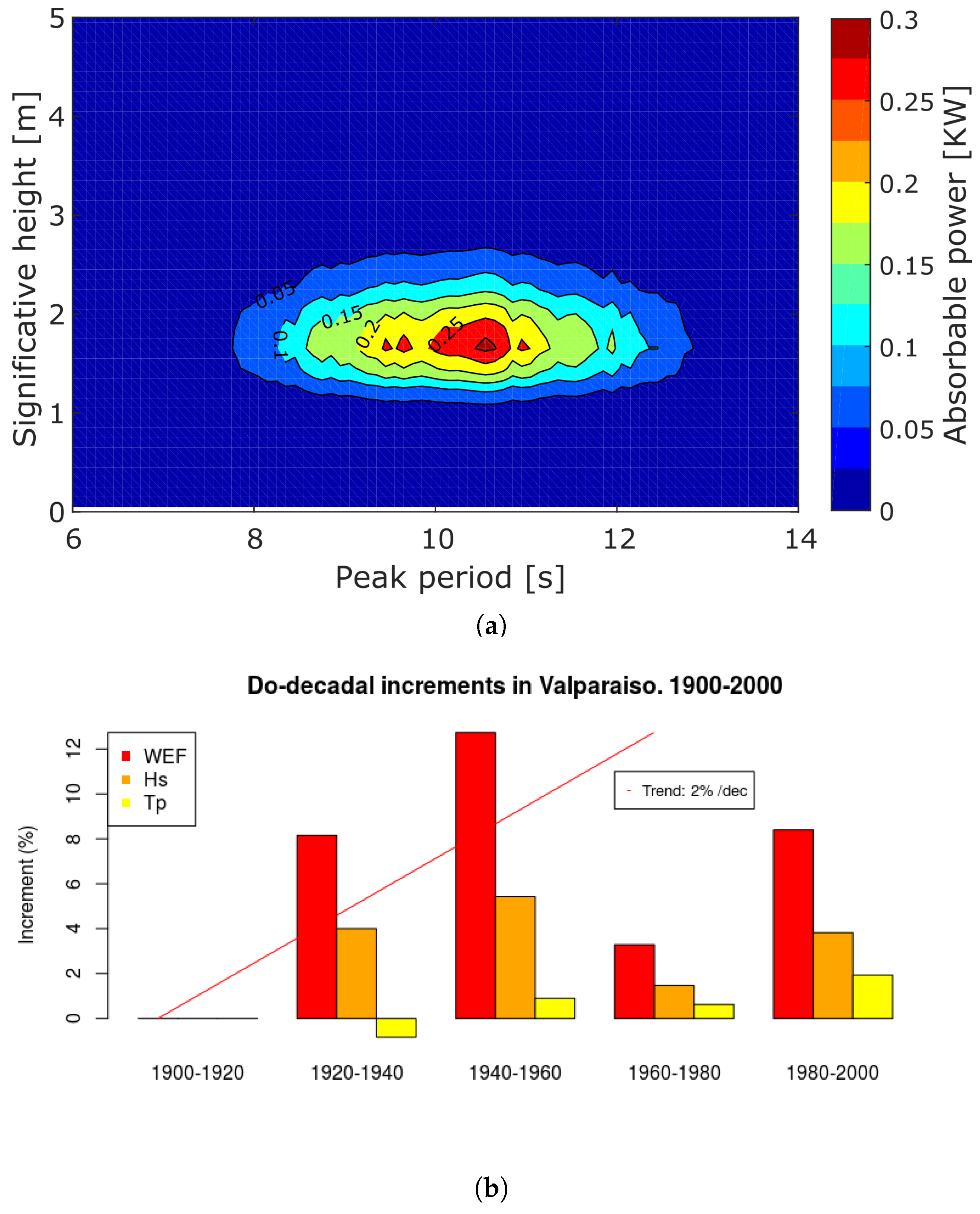
4.3.1. Wave Resource Variations

According to Figure 6, which is created using wave data from the dcERA20 model, decadal $H_s$, $T_m$ and $WEF$ trends are approximately 1.2 cm/decade, 2. 5 cs/decade and 0.4 kW/m/decade, respectively. A more detailed study, analysing each do-decade of the 20th century separately, shows that the mean $WEF$ in the first do-decade, i.e., 1900–1920, was about 19.1 kW/m/decade. Hence, the decadal $WEF$ increase of 0.4 kW/m shown in Figure 6c corresponds to a decadal increase of about 2% ($0.39/19.1\times 100=2\%$).

The scatter-diagram of the resource in this first do-decade of the 20th century is illustrated in Figure 8a, where the most frequent $H_s$ and $T_p$ are shown to be 1.5 m and 10.5 s, respectively. Wave trends of the next do-decades are shown as relative variations (in percentage) with respect to the wave resource in the first do-decade, as shown in Figure 8b, where the decadal increase of 2% is also illustrated. This general trend is consistent with other studies carried out in the same area [24,30]. However, as depicted in Figure 8b, the inter-decadal trends over the 20th century are highly irregular, with significant increases in some do-decades, between 1920 and 1960, for example, and a strong reduction in others, such as between 1960 and 1980.

The bars in Figure 8 show the increase of $WEF$, $H_s$ and $T_p$ in percentage at each do-decade, with respect to the first do-decade. These bars show a progressive increase of the wave period all over the century, while the $WEF$ and $H_s$ show more irregular patterns, with significant increases in the first two do-decades, and a very strong decrease in the fourth do-decade. The $WEF$ and $H_s$ increase again in the last do-decade. Despite the irregular variations in the different do-decades, wave energy resource variations are significantly more consistent compared to the progressive strong increases detected in the Bay of Biscay and west coast of Ireland in [7] and [8], respectively.

4.3.2. Impact on Wave Energy Absorption

The power absorbed from ocean waves by the cPA is assessed using the annual mean power production (AMPP) metric. Figure 9 illustrates the variation of the AMPP over the 20th century, if the cPA were deployed in Valparaiso. AMPP variations follow the same pattern as the $WEF$ variations, illustrated in Figure 8. However, AMPP variations are lower than resource variations. An increase of 6% in AMPP is observed in the second do-decade, with respect to the first do-decade, while the resource increases by 8%. This difference is even larger for the third do-decade, with an increase of over 12% in $WEF$, while the increase in AMPP is almost identical to the second do-decade (6%). The reason the AMPP does not increase with the $WEF$ may be the variation of the mean $T_p$ between the second and third do-decades. While $WEF$ increases in the second do-decade, the variation of the mean $T_p$ is negative, meaning that the resource shows lower wave periods, getting closer to the natural period of the cPA (5.2 s). In contrast, mean $T_p$ variation in the third do-decade is positive, which means that the mean $T_p$ moves away from the natural period of the cPA and, as a consequence, limits the increase in AMPP. Likewise, $WEF$ variation is very similar in the second and fifth do-decades, as shown in Figure 8, while the AMPP increase depicted in Figure 9 is significantly lower in the fifth do-decade. The only difference between resource variations in the second and the fifth do-decades is again the mean $T_p$, which is significantly larger in the fifth do-decade. Consequently, the same increase in $WEF$ does not involve the same increase in AMPP, illustrating the relevance of wave period variations.

5. Discussion

The wave trend results of the calibrated wave model presented in this paper for the Chilean coast are consistent with previous studies presented in the literature, either based on data from satellite altimeter [24] or reanalyses [30,31]. The particular case of Valparaiso presented in this study shows an overall $WEF$ increase of 2%/decade over the last century, while previous studies show increments of 0–3.3% from the north to the south of Chile. In any case, this general slope is important only for the validation of the calibration, since the barplot presented in Figure 8 shows that resource variations are quite irregular over the century, including relatively strong decreases between the third and the fourth do-decades. This irregular trend, without a clear uniform variation profile, contrasts the almost linear increment profile observed in the Atlantic Ocean, more specifically, in the Bay of Biscay [7] and the west coast of Ireland [8].

This non-uniform behaviour in trends over the different decades suggests that the causes of the detected variations may be complex and multiple. Although these kind of variations are often attributed to climate change [9], different, relatively unknown global mechanisms may also play an important role.

The comparison of the wave resources in the Chilean coast and the west coast of Ireland is a judicious comparison, due to their similar wave power, as shown in [14]. However, an important difference between Chile and Ireland, also pointed out in [14], is the $COV$, which is significantly greater in Ireland. In fact, results for the $COV$ presented in [14] are similar to those presented in the present study, where a longer time-period is analysed. Hence, the wave resource in Chile is shown to be significantly more consistent than the wave resource in the west coast of Ireland. However, the impact of a more consistent resource on the AMPP of WECs is not analysed in [14]. Figure 9 compares the variations of the AMPP for the same cPA in the Chilean coast and the west coast of Ireland, where AMPP variations are shown to be significantly lower in Chile, as expected. It should be noted that Valparaiso is located in the centre of Chile, while the variability of the resource (as the $WEF$) increases most in the southern latitudes [14].

Apart from the differences in resource variations and their impact on WECs’ power production capabilities, the frequency of storms is another important factor in the process of selecting the optimum location to install a WEC farm. Storms imply that WECs are shifted into survivability mode in order to protect them from structural damages, which directly affects the cost of the structure. A simple method to quantify the frequency of storms is using a maximum $H_s$ value ($H_s^{MAX}$) that delimits the operational space of the WEC, above which the WEC shifts into survivability mode. The same method is used in [68] or [8], among others. The $H_s^{MAX}=4$ m value is found to be quite restrictive in [8], where the AMPP is shown to be drastically reduced, up to 50%, compared to the unlimited case. The events where the wave resource exceeds the $H_s^{MAX}$ limit are referred to as off-limit events, and the frequency of these off-limit events is shown in Figure 10a. These off-limit events represent 20% of the resource off the west coast of Ireland at the beginning of the 20th century, which has significantly increased, up to almost 30%, by the end of the century. In contrast, using the same $H_s^{MAX}$ limitation, the off-limit events represent less than 1% of the resource in Valparaiso, which remains quite constant over the whole century.

The impact of this difference in the frequency of off-limit events on the AMPP is shown in Figure 10b, where the AMPP is shown to decrease up to a 50% off the west coast of Ireland, while only decreasing by 1% in Valparaiso. Hence, the significantly more consistent and mild wave resource in Chile represents a more attractive location, compared to Ireland, for the implementation of wave energy projects, allowing for cost minimization and facilitating deployment or maintenance operations.

The Southern areas of the Pacific Ocean lack detailed data coverage for reanalyses during the early parts of the 20th century. Even in periods relatively close in time (1985–2012), the lack of a dense coverage by observations over scarce data regions of the Pacific implies that the computations of surface heat fluxes over the Eastern Pacific show there the highest errors [69]. In long reanalysis spanning back in time to early instrumental periods, such as is the case with ERA-20CM or 20CRA, observations poorly constrain the reanalyses during early 20th Century. This is evident in the higher spread of the forcing by HadISST during 1900 versus 2000 in ERA20-CM or the lack of closure of the surface energy balance during early years over that area even though SSTs are prescribed [70]. In the case of 20CRA, there appear lacking trends of the Pacific Circulation or the Pacific-North American (PNA) pattern [71]. The smaller number of observations over the southern Pacific during early 20th Century [34] affects the ability of the ERA-20C reanalysis to simulate a realistic PNA index and other atmospheric indices before 1940. Since ocean waves are produced by atmospheric forcing at the surface, the fact that these problems due to data coverage of the early period have already been identified in the literature point that the use of bias correction techniques such as the ones used in this paper might be more important in Southern Pacific areas than in others. However, since different bias correction techniques are available [72,73], it will be interesting in the future to compare the results presented in this paper with the ones from complementary techniques.

6. Conclusions

Results of the ERA20 reanalysis of the European Centre for Medium-Range Weather Forecasts has been shown unreliable when comparing to buoy measurements. However, the directional calibration, based on the ERAI reanalysis, presented in this paper, is shown to significantly improve the results of the ERA20 reanalysis. This calibration provides reasonably reliable wave data for the whole 20th century, which allows the study of long-term wave resource variations off the Chilean coast.

Positive wave trends over the 20th century off the Chilean coast are detected in the present study, with the southern coast showing the most significant variations. However, in contrast to other locations in the Atlantic Ocean, the positive wave trend in the Chilean coast is reasonably irregular, with the strong increases of the wave resource in some do-decades and significant reductions in others. These irregular variations indicate that a straightforward attribution of these changes to climate change may be misleading and, thus, further research is needed to establish the driving mechanisms behind these trends. In addition, although long-term variations are significant, about 2kW/m/decade over the 20th century, inter- and intra-annual variations, represented by the coefficient of variation, are shown to be significantly lower than in other locations in the Atlantic Ocean.

These resource variations over the 20th century also affect the the power absorption of wave energy converters, although variations on annual mean power production do not exactly agree with the variations of the wave energy resource. Similar to the wave energy resource variations, annual mean power production variations are significantly lower in the Chilean coast than off the west coast of Ireland. In addition, the frequency of storms, for which the wave energy converters shift to survivability mode, is significantly lower in the Chilean coast (always lower than 1%), compared to the west cost of Ireland (up to 30%). This directly affects the annual mean power production of wave energy converters, and the design of different aspects of the wave energy converters, such as mooring lines, foundations and the structure.

Hence, the selection of the optimum location for the implementation of a wave energy converter farm should consider both short- and long-term variations of the wave energy resource where the farm is planned to be installed.

References

1. Falcão, A.d.O. Wave energy utilization: A review of the technologies. Renew. Sustain. Energy Rev. 2010, 14, 899–918. [Google Scholar] [CrossRef]
2. Ibarra-Berastegi, G.; Sáenz, J.; Ulazia, A.; Serras, P.; Esnaola, G.; Garcia-Soto, C. Electricity production, capacity factor, and plant efficiency index at the Mutriku wave farm (2014–2016). Ocean Eng. 2018, 147, 20–29. [Google Scholar] [CrossRef]
3. Rusu, E.; Onea, F. Estimation of the wave energy conversion efficiency in the Atlantic Ocean close to the European islands. Renew. Energy 2016, 85, 687–703. [Google Scholar] [CrossRef]
4. Carballo, R.; Sánchez, M.; Ramos, V.; Fraguela, J.; Iglesias, G. The intra-annual variability in the performance of wave energy converters: A comparative study in N Galicia (Spain). Energy 2015, 82, 138–146. [Google Scholar] [CrossRef]
5. Reguero, B.; Losada, I.; Méndez, F. A global wave power resource and its seasonal, interannual and long-term variability. Appl. Energy 2015, 148, 366–380. [Google Scholar] [CrossRef]
6. Ramos, V.; López, M.; Taveira-Pinto, F.; Rosa-Santos, P. Influence of the wave climate seasonality on the performance of a wave energy converter: A case study. Energy 2017, 135, 303–316. [Google Scholar] [CrossRef]
7. Ulazia, A.; Penalba, M.; Ibarra-Berastegi, G.; Saenz, J. Wave energy trends over the Bay of Biscay and the consequences for wave energy converters. Energy 2017, 141, 624–634. [Google Scholar] [CrossRef]
8. Penalba, M.; Ulazia, A.; Ibarra-Berastegui, G.; Ringwood, J.; Sáenz, J. Wave energy resource variation off the west coast of Ireland and its impact on realistic wave energy converters’ power absorption. Appl. Energy 2018, 224, 205–219. [Google Scholar] [CrossRef]
9. Lehmann, M.; Karimpour, F.; Goudey, C.A.; Jacobson, P.T.; Alam, M.R. Ocean wave energy in the United States: Current status and future perspectives. Renew. Sustain. Energy Rev. 2017, 74, 1300–1313. [Google Scholar] [CrossRef]
10. Alonso, R.; Jackson, M.; Santoro, P.; Fossati, M.; Solari, S.; Teixeira, L. Wave and tidal energy resource assessment in Uruguayan shelf seas. Renew. Energy 2017, 114, 18–31. [Google Scholar] [CrossRef]
11. Lisboa, R.C.; Teixeira, P.R.; Fortes, C.J. Numerical evaluation of wave energy potential in the south of Brazil. Energy 2017, 121, 176–184. [Google Scholar] [CrossRef]
12. Cruz, J.; Thomson, M.; Stavrioulia, E. Preliminary Site Selection—Chilean Marine Energy Resources. Technical Report 100513/BR/02, Garrad Hassan and Partners Limited. Available online: http://www.etymol.com/downloads/garrad_hassan_chilean_marine_energy_resources.pdf (accessed on 18 July 2018).
13. Di Lauro, E.; Contestabile, P.; Vicinanza, D. Wave Energy in Chile: A Case Study of the Overtopping Breakwater for Energy Conversion (OBREC). In Proceedings of the 12th European Wave and Tidal Energy Conference, Cork, Ireland, 27 August–1 September 2017. [Google Scholar]
14. Ringwood, J.; Brandle, G. A new world map for wave power with a focus on variability. In Proceedings of the 11th European Wave and Tidal Energy Conference, Nantes, France, 6–11 September 2015. [Google Scholar]
15. Lucero, F.; Catalán, P.A.; Ossandón, Á.; Beyá, J.; Puelma, A.; Zamorano, L. Wave energy assessment in the central-south coast of Chile. Renew. Energy 2017, 114, 120–131. [Google Scholar] [CrossRef]
16. Mediavilla, D.G.; Sepúlveda, H.H. Nearshore assessment of wave energy resources in central Chile (2009–2010). Renew. Energy 2016, 90, 136–144. [Google Scholar] [CrossRef]
17. Monárdez, P.; Acuña, H.; Scott, D. Evaluation of the potential of wave energy in Chile. In Proceedings of the ASME 2008 27th International Conference on Offshore Mechanics and Arctic Engineering, Estoril, Portugal, 15–20 June 2008; pp. 801–809. [Google Scholar]
18. WMO. Calculation of Monthly and Annual 30-year Standard Normals; WCDP-No. 10. WMO-TD/No. 341; World Metheorological Organization: Geneva, Switzerland, 1989. [Google Scholar]
19. WMO. The role of Climatological Normals in a Changing Climate; WCDMP-61, WMO-TD/1377; Word Metheorological Organization: Geneva, Switzerland, 2007. [Google Scholar]
20. Ruggiero, P.; Komar, P.D.; Allan, J.C. Increasing wave heights and extreme value projections: The wave climate of the US Pacific Northwest. Coast. Eng. 2010, 57, 539–552. [Google Scholar] [CrossRef]
21. Gulev, S.K.; Grigorieva, V. Last century changes in ocean wind wave height from global visual wave data. Geophys. Res. Lett. 2004, 31. [Google Scholar] [CrossRef] [Green Version]
22. Gulev, S.K.; Grigorieva, V. Variability of the winter wind waves and swell in the North Atlantic and North Pacific as revealed by the voluntary observing ship data. J. Clim. 2006, 19, 5667–5685. [Google Scholar] [CrossRef]
23. Woolf, D.K.; Challenor, P.; Cotton, P. Variability and predictability of the North Atlantic wave climate. J. Geophys. Res. Ocean. 2002, 107. [Google Scholar] [CrossRef] [Green Version]
24. Young, I.; Zieger, S.; Babanin, A.V. Global trends in wind speed and wave height. Science 2011, 332, 451–455. [Google Scholar] [CrossRef] [PubMed]
25. Sterl, A.; Komen, G.; Cotton, P. Fifteen years of global wave hindcasts using winds from the European Centre for Medium-Range Weather Forecasts reanalysis: Validating the reanalyzed winds and assessing the wave climate. J. Geophys. Res. Ocean. 1998, 103, 5477–5492. [Google Scholar] [CrossRef] [Green Version]
26. Cox, A.T.; Swail, V.R. A global wave hindcast over the period 1958–1997: Validation and climate assessment. J. Geophys. Res. 2001, 106, 2313–2329. [Google Scholar] [CrossRef]
27. Wang, X.L.; Zwiers, F.W.; Swail, V.R. North Atlantic ocean wave climate change scenarios for the twenty-first century. J. Clim. 2004, 17, 2368–2383. [Google Scholar] [CrossRef]
28. Wang, X.L.; Swail, V.R. Climate change signal and uncertainty in projections of ocean wave heights. Clim. Dyn. 2006, 26, 109–126. [Google Scholar] [CrossRef]
29. Bertin, X.; Prouteau, E.; Letetrel, C. A significant increase in wave height in the North Atlantic Ocean over the 20th century. Glob. Planet. Chang. 2013, 106, 77–83. [Google Scholar] [CrossRef]
30. Zheng, C.; Shao, L.; Shi, W.; Su, Q.; Lin, G.; Li, X.; Chen, X. An assessment of global ocean wave energy resources over the last 45 a. Acta Oceanol. Sin. 2014, 33, 92–101. [Google Scholar] [CrossRef]
31. Zheng, C.W.; Wang, Q.; Li, C.Y. An overview of medium- to long-term predictions of global wave energy resources. Renew. Sustain. Energy Rev. 2017, 79, 1492–1502. [Google Scholar] [CrossRef]
32. Sierra, J.; Casas-Prat, M.; Campins, E. Impact of climate change on wave energy resource: The case of Menorca (Spain). Renew. Energy 2017, 101, 275–285. [Google Scholar] [CrossRef]
33. Worley, S.J.; Woodruff, S.D.; Reynolds, R.W.; Lubker, S.J.; Lott, N. ICOADS release 2.1 data and products. Int. J. Climatol. 2005, 25, 823–842. [Google Scholar] [CrossRef] [Green Version]
34. Poli, P.; Hersbach, H.; Dee, D.P.; Berrisford, P.; Simmons, A.J.; Vitart, F.; Laloyaux, P.; Tan, D.G.; Peubey, C.; Thépaut, J.N.; et al. ERA-20C: An atmospheric reanalysis of the twentieth century. J. Clim. 2016, 29, 4083–4097. [Google Scholar] [CrossRef]
35. Dada, O.A.; Li, G.; Qiao, L.; Ma, Y.; Ding, D.; Xu, J.; Li, P.; Yang, J. Response of waves and coastline evolution to climate variability off the Niger Delta coast during the past 110 years. J. Mar. Syst. 2016, 160, 64–80. [Google Scholar] [CrossRef]
36. Patra, A.; Bhaskaran, P.K. Temporal variability in wind–wave climate and its validation with ESSO-NIOT wave atlas for the head Bay of Bengal. Clim. Dyn. 2017, 49, 1271–1288. [Google Scholar] [CrossRef]
37. Kumar, P.; Min, S.K.; Weller, E.; Lee, H.; Wang, X.L. Influence of Climate Variability on Extreme Ocean Surface Wave Heights Assessed from ERA-Interim and ERA-20C. J. Clim. 2016, 29, 4031–4046. [Google Scholar] [CrossRef]
38. Komen, G.J.; Cavaleri, L.; Donelan, M.; Hasselmann, K.; Hasselmann, S.; Janssen, P. Dynamics and Modelling of Ocean Waves; Cambridge University Press: Cambridge, UK, 1996. [Google Scholar]
39. Bidlot, J.; Janssen, P.; Abdalla, S.; Hersbach, H. A Revised Formulation of Ocean Wave Dissipation and Its Model Impact; European Centre for Medium-Range Weather Forecasts: Reading, UK, 2007. [Google Scholar]
40. Berrisford, P.; Dee, D.; Fielding, K.; Fuentes, M.; Kallberg, P.; Kobayashi, S.; Uppala, S. The ERA-Interim Archive; European Centre for Medium-Range Weather Forecasts: Reading, UK, 2009; pp. 1–16. [Google Scholar]
41. Cahill, B.; Lewis, T. Wave period ratios and the calculation of wave power. In Proceedings of the 2nd Annual Marine Energy Technology Symposium(METS 2014), Seattle, WA, USA, 15–17 April 2014. [Google Scholar]
42. Contestabile, P.; Ferrante, V.; Vicinanza, D. Wave energy resource along the coast of Santa Catarina (Brazil). Energies 2015, 8, 14219–14243. [Google Scholar] [CrossRef]
43. Block, P.; Souza Filho, F.; Sun, L.; Kwon, H.H. A streamflow forecasting framework using multiple climate and hydrological models. J. Am. Water Resour. Assoc. 2009, 45, 828–843. [Google Scholar] [CrossRef]
44. Boa, J.; Terray, L.; Habets, F.; Martin, E. Statistical and dynamical downscaling of the Seine basin climate for hydro-meteorological studies. Int. J. Climatol. 2007, 27, 1643–1655. [Google Scholar] [CrossRef] [Green Version]
45. Sun, F.; Roderick, M.L.; Lim, W.H.; Farquhar, G.D. Hydroclimatic projections for the Murray-Darling Basin based on an ensemble derived from Intergovernmental Panel on Climate Change AR4 climate models. Water Resour. Res. 2011, 47. [Google Scholar] [CrossRef] [Green Version]
46. Piani, C.; Haerter, J.O.; Coppola, E. Statistical bias correction for daily precipitation in regional climate models over Europe. Theor. Appl. Climatol. 2010, 99, 187–192. [Google Scholar] [CrossRef]
47. Rojas, R.; Feyen, L.; Dosio, A.; Bavera, D. Improving pan-European hydrological simulation of extreme events through statistical bias correction of RCM-driven climate simulations. Hydrol. Earth Sys. Sci. 2011, 15, 2599–2620. [Google Scholar] [CrossRef] [Green Version]
48. Teutschbein, C.; Seibert, J. Bias correction of regional climate model simulations for hydrological climate-change impact studies: Review and evaluation of different methods. J. Hydrol. 2012, 456, 12–29. [Google Scholar] [CrossRef]
49. Watanabe, S.; Kanae, S.; Seto, S.; Yeh, P.J.F.; Hirabayashi, Y.; Oki, T. Intercomparison of bias-correction methods for monthly temperature and precipitation simulated by multiple climate models. J. Geophys. Res. Atmos. 2012, 117. [Google Scholar] [CrossRef] [Green Version]
50. Lafon, T.; Dadson, S.; Buys, G.; Prudhomme, C. Bias correction of daily precipitation simulated by a regional climate model: a comparison of methods. Int. J. Climatol. 2013, 33, 1367–1381. [Google Scholar] [CrossRef] [Green Version]
51. Bett, P.E.; Thornton, H.E.; Clark, R.T. Using the Twentieth Century Reanalysis to assess climate variability for the European wind industry. Theor. Appl. Climatol. 2015, 1–20. [Google Scholar] [CrossRef]
52. Panofsky, H.; Brier, G. Some Applications of Statistics to Meteorology; Pennsylvania State University: University Park, PA, USA, 1958. [Google Scholar]
53. Applequist, S. Wind Rose Bias Correction. J. Appl. Meteorol. Climatol. 2012, 51, 1305–1309. [Google Scholar] [CrossRef]
54. Taylor, K.E. Summarizing multiple aspects of model performance in a single diagram. J. Geophys. Res. Atmos. 2001, 106, 7183–7192. [Google Scholar] [CrossRef] [Green Version]
55. Sen, P.K. Estimates of the regression coefficient based on Kendall’s tau. J. Am. Stat. Assoc. 1968, 63, 1379–1389. [Google Scholar] [CrossRef]
56. Theil, H. A rank-invariant method of linear and polynomial regression analysis, 3; confidence regions for the parameters of polynomial regression equations. Indagat. Math. 1950, 1, 467–482. [Google Scholar]
57. Fiévez, J.; Sawyer, T. Lessons Learned from Building and Operating a Grid Connected Wave Energy Plant. In Proceedings of the 11th European Wave and Tidal Energy Conference, Nantes, France, 6–11 September 2015. [Google Scholar]
58. Lejerskog, E.; Boström, C.; Hai, L.; Waters, R.; Leijon, M. Experimental results on power absorption from a wave energy converter at the Lysekil wave energy research site. Renew. Energy 2015, 77, 9–14. [Google Scholar] [CrossRef] [Green Version]
59. Hals, J.; Ásgeirsson, S.G.; Hjálmarsson, E.; Maillet, J.; Moller, P.; Pires, P.; Guérinel, M.; Lopes, M. Tank testing of an inherently phase controlled Wave Energy Converter. In Proceedings of the 11th European Wave and Tidal Energy Conference, Nantes, France, 6–11 September 2015. [Google Scholar]
60. Wang, W.; Wu, M.; Palm, J.; Eskilsson, C. Estimation of numerical uncertainty in computational fluid dynamics simulations of a passively controlled wave energy converter. Proc. Inst. Mech. Eng. Part M J. Eng. Marit. Environ. 2018, 232, 71–84. [Google Scholar] [CrossRef]
61. Hasselmann, K.; Barnett, T.; Bouws, E.; Carlson, H.; Cartwright, D.; Enke, K.; Ewing, J.; Gienapp, H.; Hasselmann, D.; Kruseman, P.; et al. Measurements of Wind-wave Growth and Swell Decay During the Joint North Sea Wave Project (JONSWAP); Deutsches Hydrographisches Institut: Hamburg, Germany, 1973. [Google Scholar]
62. Cummins, W. The impulse response function and ship motion. Schiffstechnik 2010, 9, 101–109. [Google Scholar]
63. Morison, J.; Johnson, J.; Schaaf, S. The force exerted by surface waves on piles. J. Petrol. Technol. 1950, 2, 149–154. [Google Scholar] [CrossRef]
64. Penalba, M.; Giorgi, G.; Ringwood, J.V. Mathematical modelling of wave energy converters: A review of nonlinear approaches. Renew. Sustain. Energy Rev. 2017, 78, 1188–1207. [Google Scholar] [CrossRef]
65. Giorgi, G.; Ringwood, J.V. A Compact 6-DoF Nonlinear Wave Energy Device Model for Power Assessment. IEEE Trans. Sustain. Energy 2018. [Google Scholar] [CrossRef]
66. Penalba, M.; Davison, J.; Windt, C.; Ringwood, J. A High-Fidelity Wave-to-Wire Model for Wave Energy Converters: Coupled numerical wave tank and power take-off models. Appl. Energy 2018, 226, 655–669. [Google Scholar] [CrossRef]
67. Babarit, A.; Hals, J.; Muliawan, M.; Kurniawan, A.; Moan, T.; Krokstad, J. Numerical benchmarking study of a selection of wave energy converters. Renew. Energy 2012, 41, 44–63. [Google Scholar] [CrossRef]
68. Mérigaud, A.; Ringwood, J.V. Power production assessment for wave energy converters: Overcoming the perils of the power matrix. Proc. Inst. Mech. Eng. Part M J. Eng. Marit. Environ. 2018, 232, 50–70. [Google Scholar] [CrossRef]
69. Liu, C.; Allan, R.P.; Berrisford, P.; Mayer, M.; Hyder, P.; Loeb, N.; Smith, D.; Vidale, P.L.; Edwards, J.M. Combining satellite observations and reanalysis energy transports to estimate global net surface energy fluxes 1985–2012. J. Geophys. Res. Atmos. 2015, 120, 9374–9389. [Google Scholar] [CrossRef]
70. Hersbach, H.; Peubey, C.; Simmons, A.; Berrisford, P.; Poli, P.; Dee, D. ERA-20CM: A twentieth-century atmospheric model ensemble. Q. J. R. Meteorol. Soc. 2015, 141, 2350–2375. [Google Scholar] [CrossRef]
71. Compo, G.P.; Whitater, J.S.; Sardeshmukh, P.D.; Matsui, N.; Allan, R.J.; Yin, X.; Gleason, B.E.; Vose, R.S.; Rutledge, G.; Bessemoulin, P.; et al. The Twentieth Century Reanalysis Project. Q. J. R. Meteorol. Soc. 2011, 137, 1–28. [Google Scholar] [CrossRef] [Green Version]
72. Kim, K.B.; Kwon, H.H.; Han, D. Bias correction methods for regional climate model simulations considering the distributional parametric uncertainty underlying the observations. J. Hydrol. 2015, 530, 568–579. [Google Scholar] [CrossRef] [Green Version]
73. Maraun, D. Bias Correcting Climate Change Simulations—A Critical review. Curr. Clim. Chang. Rep. 2016, 2, 211–220. [Google Scholar] [CrossRef]
Figure 1. The complete area of study and the exact location of the two buoys used in this study.
Energies 11 02289 g001
Figure 2. Wave roses of the two buoys: (a) Iquique; and (b) Valparaiso.
Energies 11 02289 g002
Figure 3. The illustration (a); and the power-matrix (b) of the Corpower device.
Energies 11 02289 g003
Figure 4. Taylor Diagrams for Iquique (a) and Valparaiso (b) buoys.
Energies 11 02289 g004
Figure 5. Mean values of H s (a), T m (b), W E F (c) and C O V (d) in the study area.
Energies 11 02289 g005aEnergies 11 02289 g005b
Figure 6. Trends of H s (cm/decade) (a), T m (cs/decade) (b) and W E F (kW/m/decade) (c) in the study area.
Energies 11 02289 g006
Figure 7. Wave energy trends for autumn (a), winter (b), spring (c) and summer (d).
Energies 11 02289 g007aEnergies 11 02289 g007b
Figure 8. The scatter-diagram of Valparaiso using the data for the first do-decade of the 20th century (1900–1920) (a) and the variations of the resource over the century (b).
Energies 11 02289 g008
Figure 9. AMPP variation over the 20th century in Valparaiso (Chile) and Galway bay (Ireland).
Energies 11 02289 g009
Figure 10. Occurrence of the off-limit sea-states (a) and its impact on the AMPP of the Corpower device (b) over the 20th century in Valparaiso (Chile) and Galway bay (Ireland).
Energies 11 02289 g010