On Wind Turbine Power Delta Control

IKERLAN, Po. J. M.a Arizmendiarrieta, 2, 20500 Arrasate-Mondragón, Gipuzkoa, Spain
*
Author to whom correspondence should be addressed.
Energies 2019, 12(12), 2344; https://doi.org/10.3390/en12122344
Submission received: 1 April 2019
/
Revised: 14 June 2019
/
Accepted: 14 June 2019
/
Published: 19 June 2019
(This article belongs to the Special Issue Design, Fabrication and Performance of Wind Turbines 2019)
Abstract
:One of the major challenges facing wind energy at the moment is its dependence on dispatchable energy sources to match power supply to demand and provide an adequate spinning reserve. There is no fundamental impediment for this to be done with wind energy when wind conditions are such that sufficient wind power is available. It is, in fact, common for wind farms to participate in primary and secondary frequency regulation via droop curves, curtailment, synthetic inertia, proportional de-loading, and delta control. However, although the literature presents several approaches to turbine-level control functions of this sort, it is not trivial to extract from it a readily industrializable set of algorithms. Said extraction, focused on delta control and the addition of our own contributions, is the purpose of this paper, where we propose an extension of popular torque and pitch control algorithms, which allows delta control without the wind speed observers used by other authors.
1. Introduction
We are interested in delta control algorithms, as defined by Table 1 in reference to the notation used by Aho et al. [1], because they are used by several authors for frequency control [2,3,4,5,6,7,8]. Given a de-rating command [1], the wind turbine operates with a power reserve given by Table 1.
In Mode 1, a power limit proportional to rated power is set: . In practical terms, available power is the power the turbine can generate in normal operation given the wind conditions. If is larger than , a power reserve of exists. However, said reserve is not controlled, and therefore, Mode 1 is not normally referred to as delta control [9]. We call it power limitation, after Kristoffersen [9].
In Mode 2, the power reserve is actively controlled so that it remains constant at . Obviously, this is only possible as long as . This is referred to by Kristoffersen as delta control [9]. Since, for a given value of , the desired power reserve is constant in Mode 2, we call it constant delta control, to distinguish it from Mode 3.
In Mode 3, the power reserve is actively controlled so that it remains proportional to available power, with factor . We therefore call it proportional delta control.
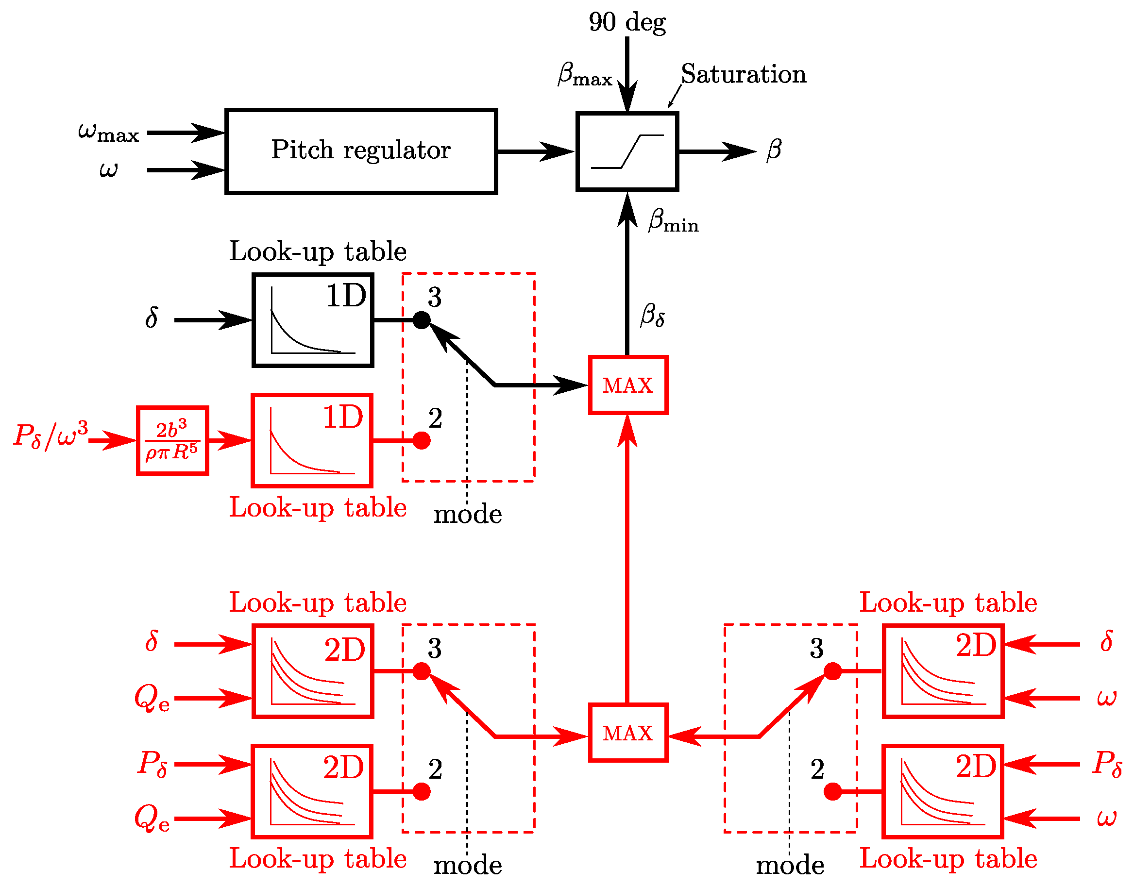
Proportional delta control has been extensively discussed in the literature. Early works, such as that of Ramtharan et al. [10], modified the maximum power point tracking (MPPT) generator speed-torque curve to track a known, sub-optimal power coefficient. This results in operating points within the turbine’s variable speed range moving to considerably higher speeds, as explained by Aho et al. [1]. A number of authors have adopted the same approach [11,12,13] and recognized that the power reserve is limited by the maximum allowable generator speed. Other authors have proposed a simple extension to the modified MPPT curve, to achieve proportional delta control via a combination of generator speed and blade pitch angle modifications [14]. This allows precise control of the tip-speed ratio and the blade pitch angle at different de-rating command values, which is relevant to turbine dynamics and loads [14,15,16,17]. Its implementation is rather simple, as shown by Figure 1 and Figure 2, where the two black 1D look-up tables are sufficient. However, as explained in Section 4.2 and Section 4.3, methods based on the MPPT curve are no longer viable when generator speed or torque limits are reached. Here, we propose an extension to said methods, which overcomes said difficulty. It is also shown by Figure 1 and Figure 2, in red. Note that it only requires two extra 2D look-up tables for proportional delta control (Mode 3), both affecting the minimum pitch on Figure 2.
Constant delta control is typically pursued via estimation of available power. This requires direct measurement of wind speed [18] or estimation thereof [1,19], with suitably slow estimator dynamics [1]. This may be considered a drawback [20]. However, an alternative exists along the lines of MPPT curve modification typical of proportional delta control techniques. Janssens et al. used a 2D look-up table [21], which gave the generator power based on the generator speed and the de-rating command. This is equivalent to substituting a 2D look-up table for the red one in Figure 1. In Section 5, we simplify this to a 1D look-up table (as shown in Figure 1) and extend it to allow control over and , as in proportional delta control (for this, we use the red 1D look-up table in Figure 2). We then extend it further to overcome generator speed and torque limitations, with the two 2D look-up tables for constant delta control (Mode 2) in Figure 2.
Section 2 reviews previous work cited here. Section 3 presents the control algorithm we wish to extend, which we subsequently extend for proportional and constant delta control in Section 4 and Section 5, respectively, on a control-region-by-control-region basis, i.e., assuming that operating points within each region (variable speed and torque, constant speed, constant torque) remain in said region regardless of the power delta. Since this is not always the case, Section 6 describes the method used here to produce look-up tables valid for any wind speed. A set of look-up tables thus produced has been used to carry out the simulations presented in Section 7 as a proof of concept. Further discussion and a detailed description of the materials and methods follow in Section 8 and Section 9, respectively.
2. Literature Review
2.1. Proportional Delta Control
Aho et al. [1] used proportional delta control (Mode 3 in their algorithm) for primary frequency control. Their technique is based on previous work by Ma and Chowdhury [22] and Juankorena et al. [23], in which a simple modification of the MPPT curve was proposed. However, Aho et al. recognized that said precedents ignored the turbine’s speed limitation and that said limitation is relevant in practice because de-rating causes a considerable increase in generator speed (they give an example in which, to produce 80% of available power, the turbine accelerates from 1000 to 1500 rpm). This effectively sets a very restrictive limit on the range of de-rating command values and wind speeds for which delta control can be achieved with their technique. They consequently made the power command proportional to available power, thus reducing a delta control problem to a power limitation problem. They estimated available power with a method by Østergaard et al. [24]. This requires considerable low-pass filtering, which results in a slow response to changes in wind speed.
Ramtharan et al. [10] also proposed the same MPPT curve modification technique above and realized the limitation imposed by the turbine’s speed limitation. They consequently applied a four degree pitch offset in order to maintain a power reserve at the maximum generator speed. This resulted in a power reserve that was not actively controlled and that was independent of the de-rating command.
De Almeida et al. [11] also proposed the same MPPT curve modification technique above, in this case without any consideration of the generator speed limits.
Zertek et al. [16] used proportional delta control to maintain an adequate power reserve for primary response to frequency events. Their technique was based on an optimization of de-rated operating points [25], for which they extended previous work [10,11] to modify the pitch angle systematically, as well as the generator speed. However, they did not consider the generator speed limits.
2.2. Constant Delta Control
Aho et al. [1] also used constant delta control (Mode 2 in their algorithm) for primary frequency control. For this, they needed a wind speed estimation for the MPPT curve modification, as well as for power limitation at the turbine’s speed limit.
Mirzaei et al. [19] proposed a model predictive control strategy for constant delta control optimization. This method required knowledge of the wind speed, for which Lio et al. proposed the use of LiDAR [18].
Zhu et al. [17] proposed a different, load-based delta control optimization at the farm level. This required the farm controller to set the turbine-level power setpoint based on wind speed.
Janssens et al. [21] proposed a modification of the MPPT curve for constant delta control. It was based on a simple 2D look-up table. The inputs to it were the desired power reserve and generator speed. The result was a method very similar to that of Ramtharan et al. [10] or de Almeida et al. [11], but it resulted in a constant power reserve, independent of the wind speed. Obviously, it suffered from the same limitations as proportional delta control methods based only on the MPPT curve modification, i.e., generator speed quickly increased with de-rating, and no reserve was possible once the maximum generator speed was reached.
3. Torque and Pitch Control
Following Jenkins et al. [26], we consider a base turbine controller with two generator speed regulators, e.g., PI controllers, one of which modifies the blades’ collective pitch angle, , while the other one modifies the generator torque .
The generator speed setpoint for the pitch controller, , was always the maximum operating speed, . The lower pitch angle saturation limit is:
where is chosen to maximize the power coefficient; we use subscript , rather than the more usual “opt” because we will use this torque for delta control in Section 4 and Section 5.
On the contrary, the generator speed setpoint for the torque controller, , is switched between and the minimum operating speed, . The choice between the two is made based on the proximity to the actual generator speed, , and the generator torque saturation limits, and , are chosen so that:
where is the rated power, while is a function of , which is chosen to make the tip-speed ratio converge to its optimal value; again, we used subscript rather than “opt”.
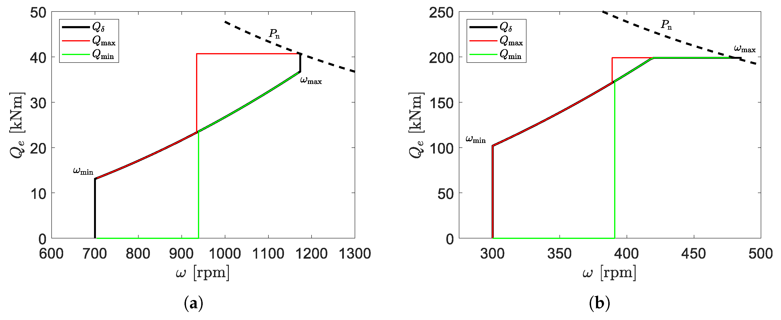
Figure 3 shows , , and for two popular reference wind turbines.
3.1. Operation at Optimal Tip-Speed Ratio
The choice of is well established, e.g., in [27]. It is based on the following simple turbine model:
where J is the rotor inertia (including the hub, drivetrain, and generator rotor), b is the gearbox ratio, is the aerodynamic torque, and is the torque due to mechanical losses.
The available aerodynamic power is:
where , R, and U are the air density, rotor radius, and wind speed, respectively, while and are the tip-speed ratio and blade pitch angle, respectively, for which the power coefficient is the greatest. Operating at is trivial; one need only choose . However, cannot be directly manipulated, or indeed measured, since it is defined as follows:
When operating at , but in general, , the aerodynamic torque is:
Equation (9) is the most common MPPT algorithm for variable-speed wind turbines [26]. It is also interesting to know whether (4), (8), and (9) lead to being asymptotically stable. To find out, we use (6) to rewrite (4), (8), and (9) thus [27]:
We then choose the following Lyapunov function candidate:
From (12), the fixed point is asymptotically stable if:
The fulfillment of these conditions may easily be verified from a turbine’s power coefficient curve, as shown by Figure 4 for two popular reference turbines.
The choice of is therefore based on (9), i.e.,
3.2. Operation at Constant Rotor Speed
Once or is reached, it is no longer possible to operate the turbine at . The tip-speed ratio at which the turbine operates now, , is determined by wind speed U, thus:
where is either or .
It is still possible, however, to choose the pitch angle, , which also influences efficiency. We are therefore interested in finding , the optimal pitch angle for the tip-speed ratio at which we are forced to operate.
When operating at , the aerodynamic torque is:
We propose the use of a look-up table giving as a function of , to set the minimum pitch saturation limit. The choice of is, therefore, made as follows:
Figure 5 shows the curves for two popular reference turbines. To calculate them, we have used Algorithm 1 for the range of wind speeds between cut-in and rated. As a result, we have two vectors for each turbine, one with pitch angles and the other with the corresponding torque values. This constitutes a usable look-up table.
| Algorithm 1 Calculate the look-up table. |
3.3. Operation at Constant Generator Torque
Larger, more powerful wind turbines operate at lower rotor speeds and, therefore, at higher torques. This may result in a turbine’s torque limit being reached before its rotational speed limit, when operating at the optimal tip-speed ratio. Such is the case, for example, of the DTU 10-MW reference wind turbine [28], if operated in “constant torque control” mode, as described in [29]. As a result, there exists a wind speed range, just below rated, in which the turbine operates at constant generator torque , yet at and . Then, instead of (17), we have:
From (6) and (19),
and because the power output is , we are interested in solutions of (20) that maximize and, therefore, . Note that this is equivalent to maximizing , for every given value of , and therefore, we are interested in using , i.e., the optimum pitch angle for a given tip-speed ratio.
We propose the use of a look-up table giving as a function of , to set the minimum pitch. The choice of is, therefore, made as follows:
Figure 6 shows the curves for two popular reference turbines. To calculate them, we have used Algorithm 2 for the range of tip-speed ratios between cut-in and rated. As a result, we have two vectors for each turbine, one with pitch angles and the other with the corresponding generator speed values. This constitutes a usable look-up table. Note, from Figure 3a, that the NREL 5-MW reference turbine does not operate at constant torque, so Figure 6a is constant at for all .
| Algorithm 2 Calculate the look-up table. |
3.4. Operation at Constant Generator Power
Power limitation at rated power is often part of the torque and pitch control described in Section 3.1. It is simply implemented by modifying (2) and (3) thus [1]:
where we have generalized to any power setting .
Note that the dynamics are the same as in Section 3.1 for , i.e., at wind speeds insufficient to reach the power setting. However, at higher wind speeds, we have, instead of (9),
Equation (25) has a fixed point at and , which satisfies:
Note that , because, although (26) has another solution at , it corresponds to generator speed , for which , and therefore, (24) does not apply.
We are, again, interested in the stability of the fixed point at , so we choose the following Lyapunov function candidate:
4. Proportional Delta Control
4.1. Proportional Delta Control with Constant Power Coefficient
Proportional delta control at certain wind speeds may easily be accomplished by modifying (14) thus [14]:
where:
Here, and are such that:
being the proportion of the available power to be kept as a reserve. This is implemented via two look-up tables, giving and , respectively, as a function of .
Note that solutions of (33) are generally non-unique, which leaves one degree of freedom for the choice of and on the basis of criteria other than those discussed here (see, for example, [15]). Figure 7 shows two different trajectories, over the contour plots of two popular reference turbines (note that the one on the right coincides exactly with Strategy 3 in [15]). The resulting and look-up tables are shown by Figure 8 and Figure 9, respectively.
4.2. Proportional Delta Control at Constant Rotor Speed
When, at higher or lower wind speeds, we are constrained to operation at , the available aerodynamic power is:
We would like to choose such that:
However, we do not know . We therefore propose extending the minimum pitch look-up table method of Section 3.2 to , via a two-dimensional look-up table giving as a function of and . Figure 10 shows said tables for two popular reference turbines and the trajectories shown by Figure 7. To calculate them, we have used Algorithm 3 for the range of wind speeds between cut-in and rated. As a result, we have two vectors for each turbine, one with de-rating command values and the other with torque values. We also have a matrix with the corresponding pitch angles. This constitutes a usable 2D look-up table.
| Algorithm 3 Calculate the look-up table. |
Note that the lines corresponding to are the same as those on Figure 5 and that the flat regions, which correspond to the interval, are as dictated by the curves on Figure 9. Note also that the considerations in Section 6 apply here and that Figure 10 has been produced via the methods described there.
4.3. Proportional Delta Control at Constant Generator Torque
When, at wind speeds just below rated, with some larger wind turbines, we are constrained to operation at (see Section 3.3), the available aerodynamic power is:
We would like to choose such that:
where is the tip-speed ratio with . However, we do not know . We therefore propose extending the minimum pitch look-up table method of Section 3.3 to , via a two-dimensional look-up table giving as a function of and . Figure 11 shows said tables for two popular reference turbines. To calculate them, we have used Algorithm 4 for the range of tip-speed ratios between cut-in and rated. As a result, we have two vectors for each turbine, one with de-rating command values and the other with generator speed values. We also have a matrix with the corresponding pitch angles. This constitutes a usable 2D look-up table.
| Algorithm 4 Calculate the look-up table. |
Note that the lines corresponding to are the same as those on Figure 6 and that the flat regions, which correspond to , are as dictated by the curves on Figure 9. Note also that the considerations in Section 6 apply here and that Figure 11 has been produced via the methods described there, where the non-flat sections on the left of Figure 11a are explained.
4.4. Proportional Delta Control at Constant Generator Power
For wind speeds above rated, it is necessary to limit to .
5. Constant Delta Control
5.1. Constant Delta Control with Variable Rotor Speed and Generator Torque
If we want to keep a constant power, , as a reserve, the choice of and may appear less obvious than in Section 4.1, because depends on , which is not directly known:
As discussed in Section 2, this is often approached by means of an estimation of . We do not discuss the merit of such means. However, a different approach is possible, based solely on a look-up table like that in Section 4.
Because (39) makes explicit reference to U, it is not directly usable without a measurement or estimation of the wind speed. We therefore rewrite (39) thus:
From (40), we would like to choose and so that:
We therefore propose using two look-up tables, giving and , respectively, as functions of . We may then use in (1) and in (31). Figure 12 and Figure 13 show said look-up tables for two popular reference turbines. To calculate them, we have used Algorithm 5 for the values on Figure 7. As a result, we have three vectors for each turbine, one with pitch angles, another with MPPT curve gains, and another with the corresponding values of ratio . This constitutes two usable look-up tables.
| Algorithm 5 Calculate the and look-up tables. |
We are, of course, interested in the dynamic characteristics of (4), (31), and (41), from which we now get, instead of (10),
There always exist and such that (41) is satisfied for and , so there is a fixed point of (42) at and . We therefore choose the following Lyapunov function candidate:
Derivation w.r.t. time and substitution of (42) yield:
From (44), the fixed point is asymptotically stable if:
Whether or not these conditions are satisfied is determined by the nature of , as shown by Figure 14 for two popular reference turbines. Note that the fixed points, which correspond with the crossing of each black line with its red counterpart, follow the trajectories shown by the red lines on Figure 7, i.e., they move from to around , as changes from 0 to 1, on Figure 14a, while they remain at on Figure 14b. Note also that all black lines turn sharply up at lower , when the trajectories on Figure 7 reach .
5.2. Constant Delta Control at Constant Rotor Speed
When, at higher or lower wind speeds, we are constrained to operation at , we would like to choose so that, instead of (41),
However, we do not know . We therefore propose using a two-dimensional look-up table giving as a function of and . Figure 15 shows said tables for two popular reference turbines and the trajectories shown by Figure 7. To calculate them, we have used Algorithm 6 for the range of wind speeds between cut-in and rated. As a result, we have two vectors for each turbine, one with de-rating command values and the other with torque values. We also have a matrix with the corresponding pitch angles. This constitutes a usable 2D look-up table.
| Algorithm 6 Calculate the look-up table. |
5.3. Constant Delta Control at Constant Generator Torque
When, at wind speeds just below rated, with some larger wind turbines, we are constrained to operation at (see Section 3.3), we would like to choose so that, instead of (37),
where is the tip-speed ratio with . However, we do not know or . We therefore propose extending the minimum pitch look-up table method of Section 3.3 to , via a two-dimensional look-up table giving as a function of and . Figure 16 shows said tables for two popular reference turbines. To calculate them, we have used Algorithm 7 for the range of tip-speed ratios between cut-in and rated. As a result, we have two vectors for each turbine, one with de-rating command values and the other with generator speed values. We also have a matrix with the corresponding pitch angles. This constitutes a usable 2D look-up table.
| Algorithm 7 Calculate the look-up table. |
5.4. Constant Delta Control at Constant Generator Power
For wind speeds above rated, it is necessary to limit to .
6. Look-Up Table Calculation
We have discussed, in Section 4, a proportional delta control method based on two 1D look-up tables (for and , respectively) within the unconstrained generator speed and torque operating region (which coincides with the region of optimal tip-speed ratio when ) and two 2D look-up tables (for and , respectively) for the generator speed- or torque-constrained operating regions. This description also applies to the constant delta control method discussed in Section 5, with instead of . There are, however, some wind speeds, near the boundaries between said operating regions, at which a wind turbine will operate in a different region depending on or .
Consider, for example, a turbine that does delta control via over-speed, as is the case of the NREL 5-MW reference turbine here, as shown by Figure 7a. Consider also a wind speed at which said turbine operates at generator speed when . Then, there is a over which said turbine, at said wind speed, must operate at generator speed . If the pitch angle is such that, at said generator speed, , then power output will be more than -times the power output at , because at generator speed for any .
The same thing happens to all over-speed-based delta control methods, which always run into for large enough , where no more over-speed is possible. Pitch-based delta control is necessary then (hence, for example, Ramtharan et al.’s four degree pitch offset [10]).
In this section, we will discuss a method to calculate the look-up tables introduced in Section 4 and Section 5 so that they are valid for any wind speed, regardless of the operating point moving between regions, as just described. The method is described by Algorithm 8.
| Algorithm 8 Calculate the look-up tables. |
|
Once the steps of Algorithm 8 have been carried out for the range of wind speeds of interest, one is left with three vectors, with the values of , , and corresponding to different wind speeds and one value of or . Repeating for different values of or , these vectors become matrices, and the 2D look-up tables giving and or and are ready. Figure 10, Figure 11, Figure 15 and Figure 16 show said tables for two popular reference turbines.
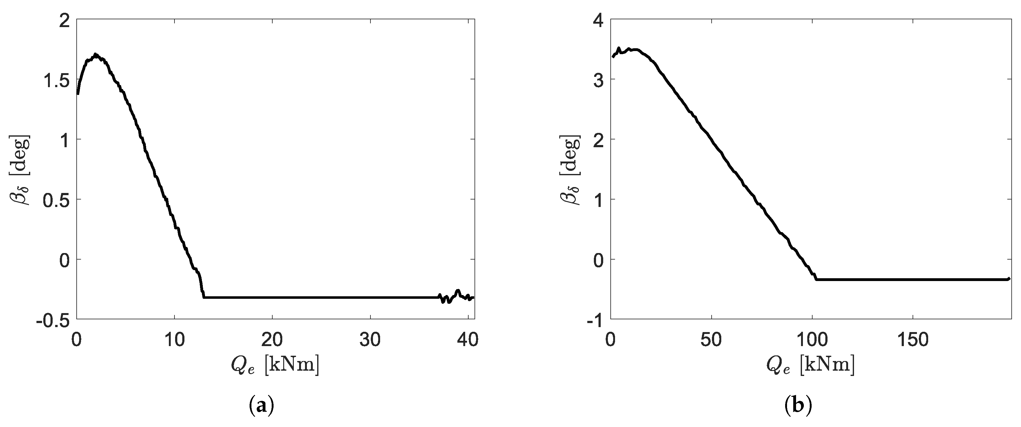
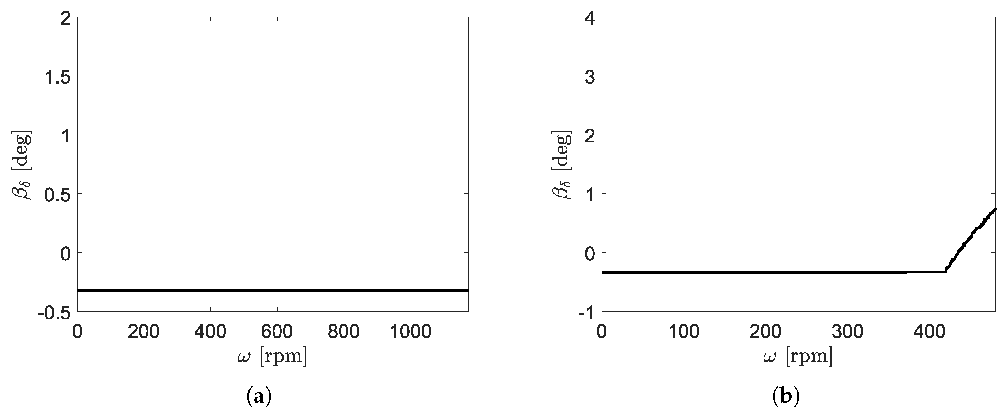
It is also possible to interpret the results of Algorithm 8 as tables giving or , as shown by Figure 17 and Figure 18. These are indeed the steady state operating points we expect from the application of the control algorithms described in this paper, but they are not used in said algorithms directly. Instead, is influenced via in (22) and (23). is calculated via (31), which uses . 1D look-up tables for and are given by Figure 8 and Figure 12, respectively.
7. Results
In order to preliminarily test the methods proposed in this paper, it is easiest for us to modify a free controller slightly [30], which we have recently produced for a research project. It was adapted to the DTU 10-MW reference wind turbine [28]. As a first proof of concept, we carried out some simulations with said controller and turbine model, which had constant speed and constant torque operating regions. This allowed us to assess the performance of all our methods at a glance, provided that we used a wide enough range of wind speeds. Unfortunately, we had no similar code for the NREL 5-MW reference wind turbine [31], and it would be inefficient for us to produce one at the time of writing.
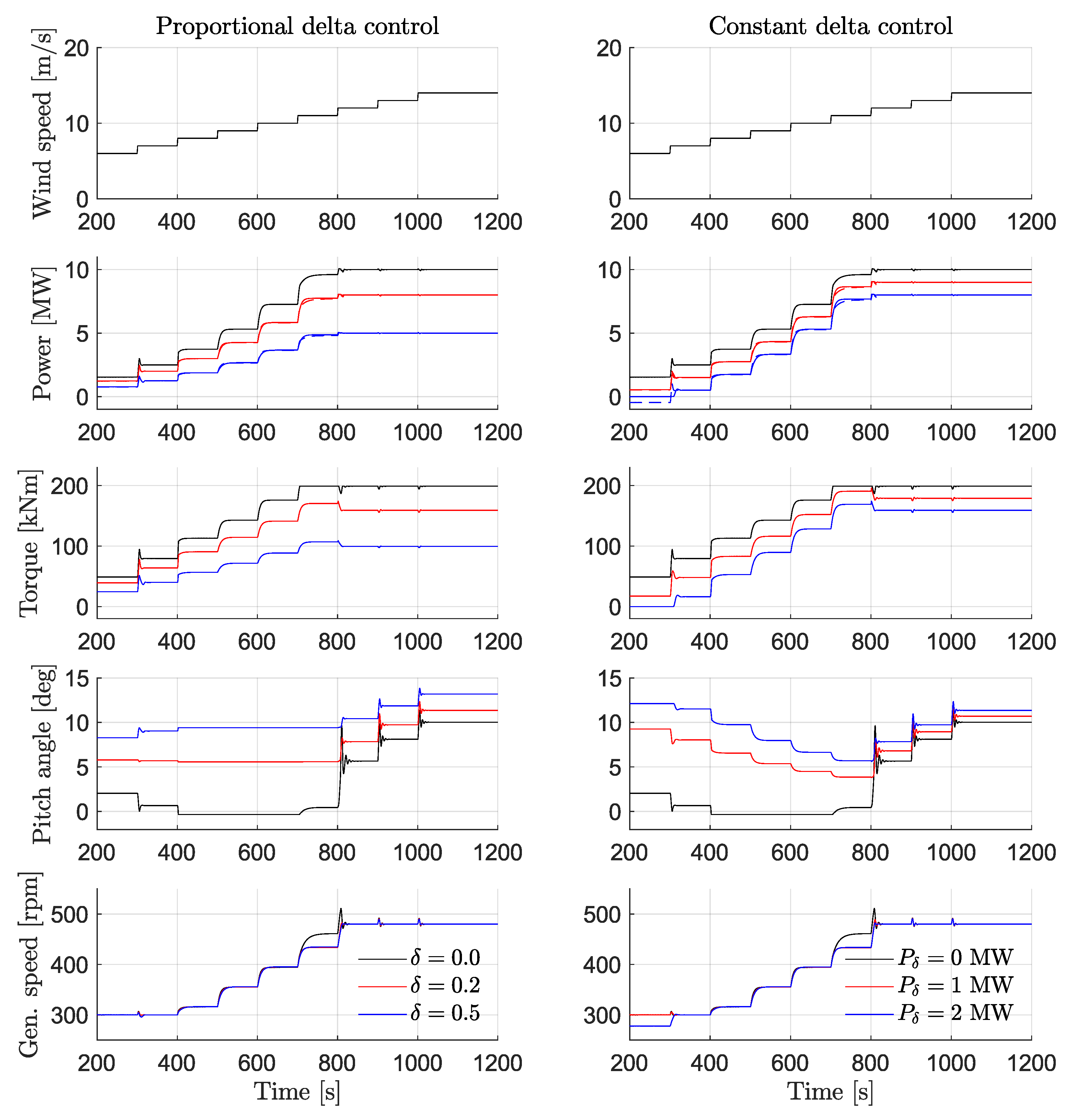
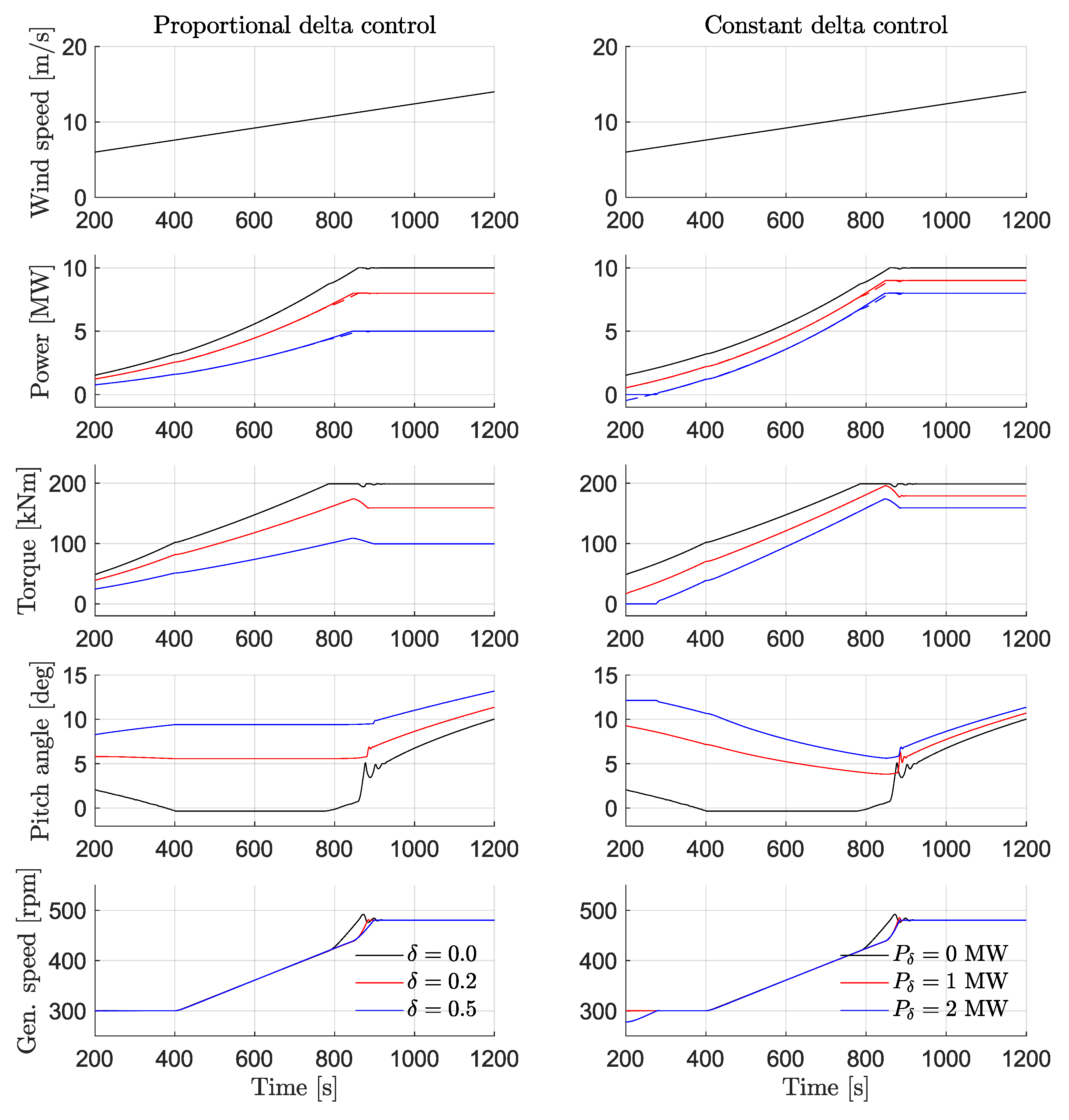
Figure 19, Figure 20 and Figure 21 show six FAST [32] simulations of the DTU 10-MW [28] reference wind turbine. Three of them were carried out with proportional, the other three with constant delta control. In each case, three different power deltas (including zero) were used. The power output of simulations corresponding to and , multiplied by and minus , respectively, are plotted in dashed lines for other values of and .
In Figure 19, the wind speed increased suddenly by 1 m/s every 100 s, so we can assess the turbine’s steady state behavior at different operating points. Prior to 400 s, the wind speed was low enough to force the turbine to work at the minimum generator speed (300 rpm). Note that, for , the generator speed was lower prior to the 300-s mark. This is because the available power was less than and suggests a further change to the control strategy, as discussed briefly in Section 8.
Between the 400-s and 500-s marks, the steady-state generator speed remained proportional to wind speed, because the trajectory on Figure 7b dictates a constant tip-speed ratio.
Between the 700-s and 800-s marks, the turbine worked at the maximum torque (198 kNm) for and , and the generator accelerated above the optimal tip-speed ratio. After the 800-s mark, the generator worked at the maximum speed for all values of and .
In all cases (except, as already pointed out, when was larger than available power, prior to the 300-s mark), the delta control behavior was excellent, as indicated by the dashed and continuous lines being very close to each other. However, an appreciable transient error appeared after the 700-s mark, due to the generator accelerating more for and than for other values of and . This also suggests a further change to the control strategy, as discussed briefly in Section 8.
In Figure 20, the wind speed slowly increased during the simulations, in order to visualize quasi-steady-state turbine behavior easily over a wide range of wind speeds. Again, the delta control behavior was excellent, except for the case of constant delta control at low wind speeds, where not enough aerodynamic power was available for a 2-MW power reserve; as a consequence, power output remained at 0 and generator speed was too low. Note also that, after the 800-s mark, there was an appreciable power delta error. This was because the generator speed was different for different de-rating commands, as was the case between the 700-s and 800-s marks on Figure 19.
In Figure 21, a turbulent wind field produced via TurbSim [33] was used. The mean wind speed was approximately 9 m/s, and the turbulence intensity was 30% (which is considerably larger than the standard [34]), so that a wide range of wind velocities may be covered within a single simulation. Note that, despite the high turbulence, the delta control behavior remained excellent. Again, as on Figure 19 and Figure 20, appreciable transient power delta errors appeared when the and simulations reached the maximum torque, due to generator speed being different for different de-rating command values. Additionally, in the simulation, the controller could not maintain the minimum generator speed when the wind speed was so low that a 2-MW reserve was impossible (around the 500-s mark). As mentioned above, these shortcomings suggest further changes to our delta control technique, which we briefly discuss in Section 8.
Finally, it is noticeable that the power delta error was slightly larger when the power output was decreasing, while it was practically perfect when the power output was increasing. This may merit further investigation.
8. Discussion
It appears, from the results presented in Section 7, that the delta control algorithms discussed in Section 4 and Section 5 work as expected, at least for the DTU 10-MW reference turbine, which we have used for our proof of concept in the wake of our work on the H2020 project CL-Windcon (see the section on funding). This leaves us with a turbine control algorithm based on three look-up tables, one of which is 1D, the other two 2D, and a method for calculating said look-up tables from a turbine’s power coefficient and operational limits, with one design freedom: the trajectory necessary for Step 12 in Section 6. Said trajectory affects several aspects of turbine control:
- Over-speed-based strategies, such as the one shown on Figure 7a, require a change of rotor speed for a change of or , which results in power transients to be studied. Specifically, the rotor speed reduction coming from the reduction of the power reserve (due to part of said reserve being summoned) during, for example, a grid under-frequency event, provides an extra energy reserve, comprised of the reduction in the rotor’s kinetic energy. How to best extract and exploit said energy is an interesting topic, strongly related to synthetic inertia methods, for future research.
- Purely pitch-based strategies, such as the one shown on Figure 7b, result in the turbine’s operating speed being independent of or for most wind speeds, as shown by Figure 20. This probably minimizes power transients due to changes in the power reserve. Note, however, from Figure 20, that the constant delta control is unable, when the wind speed is insufficient to maintain the required power reserve, to maintain generator speed at . This suggests a change in the control algorithm, according to which the generator speed setpoint for the pitch controller would be switched between and , like the setpoint for the torque controller . This would allow the pitch controller to maintain generator speed at at low wind speeds, when generator torque is saturated at zero due to being larger than available power.
- As mentioned in Section 7, strategies that result in different generator speeds for different de-rating commands result in transient power reserve errors due to changes in wind speed. This is necessarily the case in the constant torque region (Section 4.3 and Section 5.3) with the technique proposed here. It may be interesting to modify said technique to ensure that the turbine’s operating speed is independent of or for all wind speeds.
- Pitch actions due to the and (or and ) look-up tables may have relevant effects on the pitch actuator’s duty cycle and on the generator speed regulators. It is interesting to study said effects, as well as the influence of the trajectory on them.
9. Materials and Methods
NREL’s FAST [32] was used to calculate values and perform simulations. Wind turbine model data for the NREL 5-MW [35] and DTU 10-MW [28] reference turbines were taken from [31] and [36], respectively. OpenDiscon [30] commits c7c155629ee4767b8ac6176c9c3c86ecd0f82107 and 8abdf3d4d884a549e31aa8c3c803933149cdd1d7 have been used for proportional and constant delta control, respectively, in the simulations of Section 7.
Author Contributions
Conceptualization, methodology, software, validation, formal analysis, investigation, resources, data curation, visualization, and writing, original draft preparation, I.E.; writing, review and editing, supervision, project administration, and funding acquisition, I.E., C.C., and A.P.-A.
Funding
This project has received funding from the European Union’s Horizon 2020 research and innovation program under Grant Agreement No. 727477.
Conflicts of Interest
The authors declare no conflict of interest.
References
- Aho, J.; Pao, L.; Fleming, P. An Active Power Control System for Wind Turbines Capable of Primary and Secondary Frequency Control for Supporting Grid Reliability. In Proceedings of the 51st AIAA Aerospace Sciences Meeting including the New Horizons Forum and Aerospace Exposition 2013, Grapevine, TX, USA, 7–10 January 2013. [Google Scholar]
- Ahmadyar, A.S.; Verbič, G. Coordinated Operation Strategy of Wind Farms for Frequency Control by Exploring Wake Interaction. IEEE Trans. Sustain. Energy 2017, 8, 230–238. [Google Scholar] [CrossRef]
- Golden, R.; Paulos, B. Curtailment of Renewable Energy in California and Beyond. Electr. J. 2015, 28, 36–50. [Google Scholar] [CrossRef]
- Tsili, M.; Papathanassiou, S. Review of grid code technical requirements for wind farms. IET Renew. Power Gener. 2009, 3, 308–332. [Google Scholar] [CrossRef]
- Martínez de Alegría, I.; Andreu, J.; Martín, J.; Ibañez, P.; Villate, J.; Camblong, H. Connection requirements for wind farms: A survey on technical requirements and regulation. Renew. Sustain. Energy Rev. 2007, 11, 1858–1872. [Google Scholar] [CrossRef]
- Danish Energy Authority. Wind Turbines Connected to Grids with Voltages above 100 kV—Technical Regulation for the Properties and the Regulation of Wind Turbines. 2004. Available online: https://en.energinet.dk/-/media/1196EE254B854D21AD88B2DC813BFEA9.pdf (accessed on 18 June 2019).
- Siemens. Active Power Control in Wind Parks. 2011. Available online: https://www.bpa.gov/Doing%20Business/TechnologyInnovation/ConferencesVoltageControlTechnical/ActivePowerControlinWindParks_Siemens.pdf (accessed on 10 September 2018).
- Díaz-González, F.; Hau, M.; Sumper, A.; Gomis-Bellmunt, O. Participation of wind power plants in system frequency control: Review of grid code requirements and control methods. Renew. Sustain. Energy Rev. 2014, 34, 551–564. [Google Scholar] [CrossRef]
- Kristoffersen, J.R. The Horns Rev Wind Farm and the Operational Experience with the Wind Farm Main Controller; Copenhagen Offshore Wind: Copenhagen, Denmark, 2005. [Google Scholar]
- Ramtharan, G.; Ekanayake, J.B.; Jenkins, N. Frequency support from doubly fed induction generator wind turbines. IET Renew. Power Gener. 2007, 1, 3–9. [Google Scholar] [CrossRef]
- De Almeida, R.G.; Pecas Lopes, J.A. Participation of Doubly Fed Induction Wind Generators in System Frequency Regulation. IEEE Trans. Power Syst. 2007, 22, 944–950. [Google Scholar] [CrossRef] [Green Version]
- Vidyanandan, K.V.; Senroy, N. Primary frequency regulation by deloaded wind turbines using variable droop. IEEE Trans. Power Syst. 2013, 28, 837–846. [Google Scholar] [CrossRef]
- Loukarakis, E.; Margaris, I.; Moutis, P. Frequency control support and participation methods provided by wind generation. In Proceedings of the 2009 IEEE Electrical Power Energy Conference (EPEC), Montreal, QC, Canada, 22–23 October 2009; pp. 1–6. [Google Scholar] [CrossRef]
- Astrain-Juangarcia, D.; Eguinoa, I.; Knudsen, T. Derating a single wind farm turbine for reducing its wake and fatigue. J. Phys. Conf. Ser. 2018, 1037, 032039. [Google Scholar] [CrossRef]
- Van der Hoek, D.; Kanev, S.; Engels, W. Comparison of Down-Regulation Strategies for Wind Farm Control and their Effects on Fatigue Loads. In Proceedings of the 2018 Annual American Control Conference (ACC), Milwaukee, WI, USA, 27–29 June 2018; pp. 3116–3121. [Google Scholar] [CrossRef]
- Zertek, A.; Verbič, G.; Pantos, M. A Novel Strategy for Variable-Speed Wind Turbines’ Participation in Primary Frequency Control. IEEE Trans. Sustain. Energy 2012, 3, 791–799. [Google Scholar] [CrossRef]
- Zhu, J.; Ma, K.; Soltani, M.; Hajizadeh, A.; Chen, Z. Comparison of loads for wind turbine down-regulation strategies. In Proceedings of the 11th Asian Control Conference (ASCC), Gold Coast, QLD, Australia, 17–20 December 2017; pp. 2784–2789. [Google Scholar] [CrossRef]
- Lio, A.W.H.; Mirzaei, M.; Larsen, G.C. On wind turbine down-regulation control strategies and rotor speed set-point. J. Phys. Conf. Ser. 2018, 1037, 032040. [Google Scholar] [CrossRef] [Green Version]
- Mirzaei, M.; Soltani, M.; Poulsen, N.; Niemann, H. Model based active power control of a wind turbine. In Proceedings of the American Control Conference, Portland, OR, USA, 4–6 June 2014; pp. 5037–5042. [Google Scholar] [CrossRef]
- Attya, A.; Dominguez-Garcia, J.; Anaya-Lara, O. A review on frequency support provision by wind power plants: Current and future challenges. Renew. Sustain. Energy Rev. 2018, 81, 2071–2087. [Google Scholar] [CrossRef] [Green Version]
- Janssens, N.A.; Lambin, G.; Bragard, N. Active Power Control Strategies of DFIG Wind Turbines. In Proceedings of the 2007 IEEE Lausanne Power Tech, Lausanne, Switzerland, 1–5 July 2007; pp. 516–521. [Google Scholar] [CrossRef]
- Ma, H.T.; Chowdhury, B.H. Working towards frequency regulation with wind plants: Combined control approaches. IET Renew. Power Gener. 2010, 4, 308–316. [Google Scholar] [CrossRef]
- Juankorena, X.; Esandi, I.; Lopez, J.; Marroyo, L. Method to enable variable speed wind turbine primary regulation. In Proceedings of the 2009 International Conference on Power Engineering, Energy and Electrical Drives, Lisbon, Portugal, 18–20 March 2009; pp. 495–500. [Google Scholar] [CrossRef]
- Østergaard, K.Z.; Brath, P.; Stoustrup, J. Estimation of effective wind speed. J. Phys. Conf. Ser. 2007, 75, 012082. [Google Scholar] [CrossRef]
- Žertek, A.; Verbič, G.; Pantoš, M. Optimised control approach for frequency-control contribution of variable speed wind turbines. IET Renew. Power Gener. 2012, 6, 17–23. [Google Scholar] [CrossRef]
- Jenkins, N.; Burton, A.; Sharpe, D.; Bossanyi, E. Wind Energy Handbook; Wiley: Chichester, West Sussex, UK, 2001. [Google Scholar]
- Johnson, K.E. Adaptive Torque Control of Variable Speed Wind Turbines; National Renewable Energy Laboratory (NREL): Golden, CO, USA, 2004. [Google Scholar]
- Christian, B.; Frederik, Z.; Robert, B.; Taeseong, K.; Anders, Y.; Lars, C.H.; Anand, N.; Morten, H. Description of the DTU 10 MW Reference Wind Turbine; DTU Wind Energy Report-I-0092; DTU Wind Energy: Roskilde, Denmark, 2013. [Google Scholar]
- Morten Hartvig, H.; Lars Christian, H. Basic DTU Wind Energy Controller; DTU Wind Energy E-0028; DTU Wind Energy: Roskilde, Denmark, 2013. [Google Scholar]
- OpenDiscon. Available online: https://github.com/ielorza/OpenDiscon (accessed on 18 June 2019).
- Jonkman, J. Available online: https://wind.nrel.gov/public/jjonkman/ (accessed on 10 September 2018).
- FAST. Available online: https://nwtc.nrel.gov/FAST (accessed on 10 September 2018).
- TurbSim. Available online: https://nwtc.nrel.gov/TurbSim (accessed on 10 September 2018).
- Wind Turbine Generator Systems—Part 1: Safety Requirements, 2nd ed.; IEC 61400-1; IEC: Geneva, Switzerland, 1999.
- Jonkman, J.; Butterfield, S.; Musial, W.; Scott, G. Definition of a 5MW Reference Wind Turbine for Offshore System Development; National Renewable Energy Laboratory (NREL): Golden, CO, USA, 2009. [Google Scholar]
- The DTU 10MW Reference Wind Turbine Project Site. Available online: http://dtu-10mw-rwt.vindenergi.dtu.dk (accessed on 10 September 2018).
Figure 1.
MPPT curve modification for delta control (our extension in red).

Figure 2.
Minimum pitch modification for delta control (our extension in red).

Figure 3.
Generator speed-torque curves of NREL 5-MW (a) and DTU 10-MW (b) reference turbines.

Figure 4.
Optimal tip-speed ratio stability criterion for NREL 5-MW (a) and DTU 10-MW (b) reference turbines.
Figure 4.
Optimal tip-speed ratio stability criterion for NREL 5-MW (a) and DTU 10-MW (b) reference turbines.

Figure 5.
Optimal minimum pitch angle as a function of generator torque for NREL 5-MW (a) and DTU-10 MW (b) reference turbines.
Figure 5.
Optimal minimum pitch angle as a function of generator torque for NREL 5-MW (a) and DTU-10 MW (b) reference turbines.

Figure 6.
Optimal minimum pitch angle as a function of generator speed for NREL 5-MW (a) and DTU 10-MW (b) reference turbines.
Figure 6.
Optimal minimum pitch angle as a function of generator speed for NREL 5-MW (a) and DTU 10-MW (b) reference turbines.

Figure 7.
Power coefficients of NREL 5-MW (a) and DTU 10-MW (b) reference turbines.

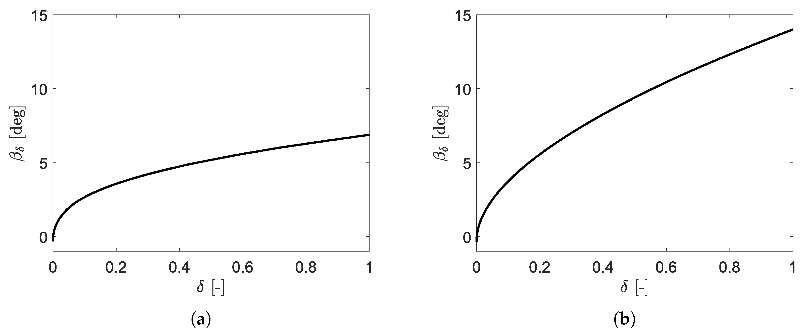
Figure 8.
tables for NREL 5-MW (a) and DTU 10-MW (b) reference turbines.

Figure 9.
tables for NREL 5-MW (a) and DTU 10-MW (b) reference turbines.

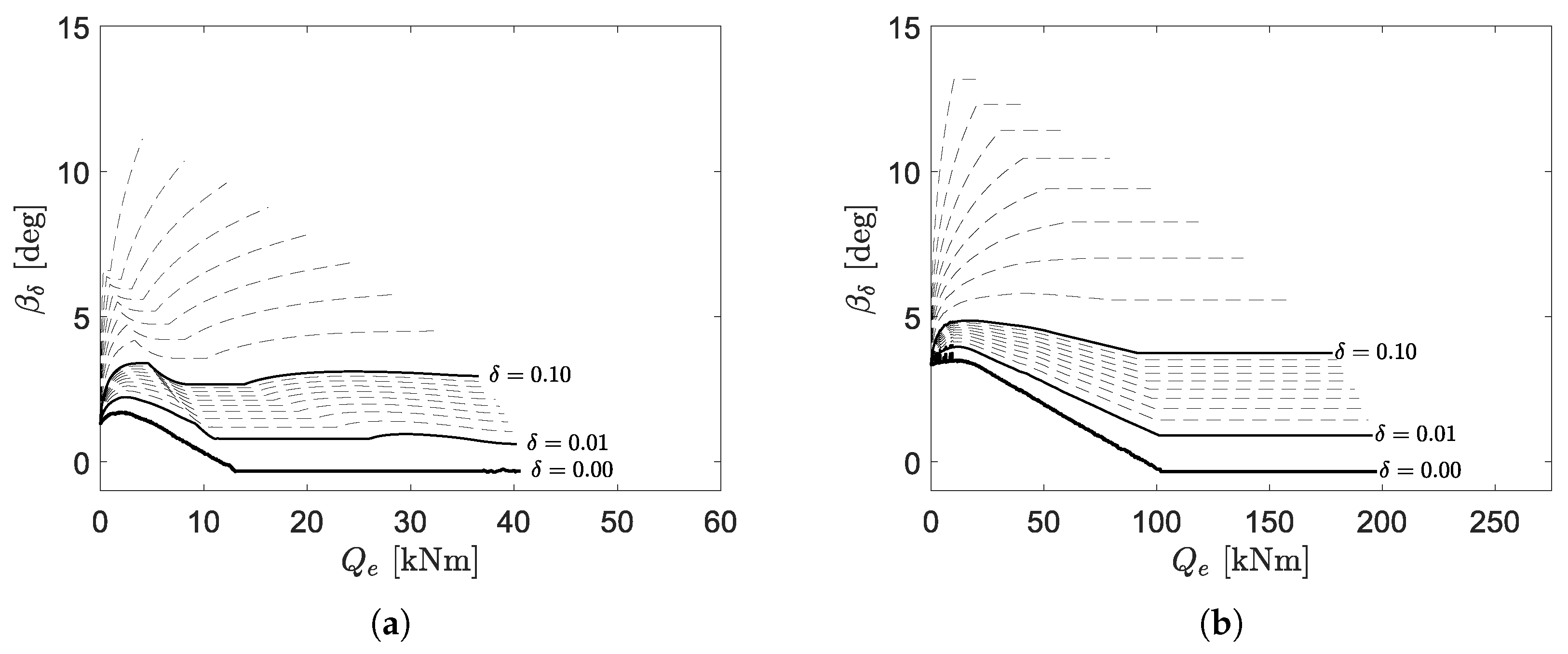
Figure 10.
tables for NREL 5-MW (a) and DTU 10-MW (b) reference turbines.

Figure 11.
tables for NREL 5-MW (a) and DTU 10-MW (b) reference turbines.

Figure 12.
tables for NREL 5-MW (a) and DTU-10 MW (b) reference turbines.

Figure 13.
tables for NREL 5-MW (a) and DTU 10-MW (b) reference turbines.

Figure 14.
Constant delta control stability criterion for NREL 5-MW (a) and DTU 10-MW (b) reference turbines, with variable generator speed and torque.
Figure 14.
Constant delta control stability criterion for NREL 5-MW (a) and DTU 10-MW (b) reference turbines, with variable generator speed and torque.

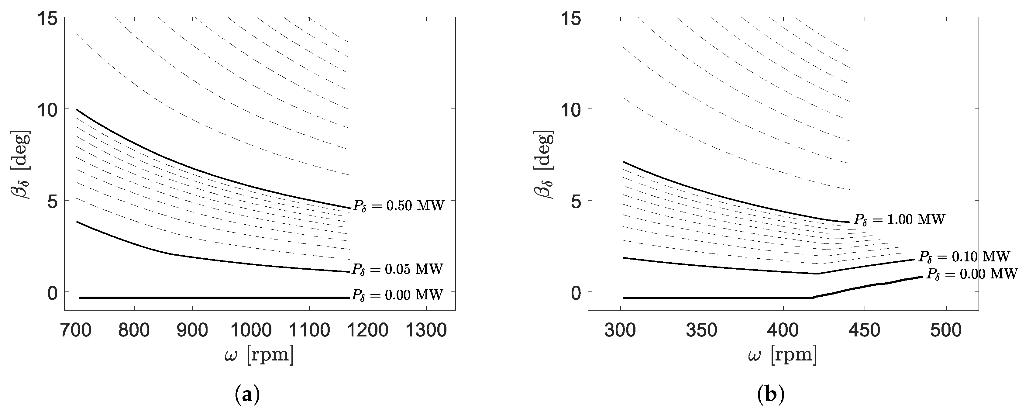
Figure 15.
tables for NREL 5-MW (a) and DTU 10-MW (b) reference turbines.

Figure 16.
tables for NREL 5-MW (a) and DTU 10-MW (b) reference turbines.

Figure 17.
tables for NREL 5-MW (a) and DTU 10-MW (b) reference turbines.

Figure 18.
tables for NREL 5-MW (a) and DTU 10-MW (b) reference turbines.

Figure 19.
DTU 10-MW reference turbine with proportional and constant delta control, wind speed steps.
Figure 19.
DTU 10-MW reference turbine with proportional and constant delta control, wind speed steps.

Figure 20.
DTU 10-MW reference turbine with proportional and constant delta control, wind speed ramp.
Figure 20.
DTU 10-MW reference turbine with proportional and constant delta control, wind speed ramp.

Figure 21.
DTU 10-MW reference turbine with proportional and constant delta control, turbulent wind field.
Figure 21.
DTU 10-MW reference turbine with proportional and constant delta control, turbulent wind field.


Table 1.
Power reserve levels resulting from the de-rating command modes in [1].
© 2019 by the authors. Licensee MDPI, Basel, Switzerland. This article is an open access article distributed under the terms and conditions of the Creative Commons Attribution (CC BY) license (http://creativecommons.org/licenses/by/4.0/).
Share and Cite
MDPI and ACS Style
Elorza, I.; Calleja, C.; Pujana-Arrese, A. On Wind Turbine Power Delta Control. Energies 2019, 12, 2344. https://doi.org/10.3390/en12122344
AMA Style
Elorza I, Calleja C, Pujana-Arrese A. On Wind Turbine Power Delta Control. Energies. 2019; 12(12):2344. https://doi.org/10.3390/en12122344
Chicago/Turabian StyleElorza, Iker, Carlos Calleja, and Aron Pujana-Arrese. 2019. "On Wind Turbine Power Delta Control" Energies 12, no. 12: 2344. https://doi.org/10.3390/en12122344
Note that from the first issue of 2016, this journal uses article numbers instead of page numbers. See further details here.