Modeling Phase Shifters in Power System Simulations Based on Reduced Networks ^†

Abstract

Phase shifters are becoming widespread assets operated by transmission system operators to deal with congestions and contingencies using non-costly remedial actions. The setting of these controllable devices, which impacts power flows over large areas, may vary significantly according to the operational conditions. It is thus a key challenge to model phase shifters appropriately in power system simulation. In particular, accounting for the flexibility of phase shifters in reduced network models is a vibrant issue, as system stakeholders rely more and more on reduced models to perform studies supporting operational and investment decisions. Different approaches in the literature are proposed to model phase shifters in reduced network. Nevertheless, these approaches are based on the electrical parameters of the system which are not suitable for reduced network models. To address this problem, our paper proposes a methodology and assesses the impact of this contribution in terms of accuracy of the modelling on reduced network models. The approach was applied to a realistic case-study of the European transmission network that was clustered into a reduced network consisting of 54 buses and 82 branches. The reduction was performed using classical clustering methods and represented using a static power transfer distribution factor matrix. The simulations highlight that including an explicit phase shifter transformers representation in reduced models is of interest, when comparing with the representation using only a static power transfer distribution factor matrix.

1. Introduction

To deal with increasing uncertainty in system operation, Transmission System Operators (TSOs) rely more and more frequently on power flow control devices, such as Phase-Shifter Transformers (PSTs) or High-Voltage Direct Current (HVDC) links. These can be used as non-costly remedial actions to solve congestions by redirecting power flows, while avoiding redispatching or countertrading or in the longer-term the costly reinforcement of the network. It is therefore important to consider those assets appropriately when performing simulation of complex processes in large-scale power systems. As such, simulations are most frequently based on a simplified representation of the network (e.g., [1,2,3]), and modeling phase shifters in reduced networks has become a vibrant issue. Indeed, reduced networks generally aim to reflect the main steady-state features of the full system (e.g., [4]), but most studies perform static reductions based on a single operation point and therefore do not consider potential setting variations for the power flow control devices [5,6]. In [7], the authors considered multiple operation points in network reduction, but ended up with a reduced model based on static Power Transfer Distribution Factors (PTDF), independent of the setting of power flow control devices.

Different approaches are proposed in the literature to model a PST in load flow computations, either by modeling the PST as an impedance in series with an ideal transformer that varies with the tap angle [8], or by modeling its impact as an injected power, using a phase-shifter distribution factor (PSDF) matrix that establishes a relationship between the injected power and flow distribution through other network elements [9]. A limitation for these kinds of approaches is the need to know the electrical parameters of the system, namely lines’ impedances or buses’ angles. This can be a challenge when dealing with reduced network models, which can often be described using a PTDF matrix only.

To address this problem, this paper proposes a methodology to emulate and assess the impact of PSTs in reduced network models. In the reduced model, PSTs are represented as an extra variable that can be adjusted subject to the systems operating point, whereas the other network components are represented by a static PTDF matrix defined with the methodology presented in [7]. To assess the proposed methodology, multiple scenarios considering different operating conditions in both the reduced and complete models are simulated and branches’ power flows are compared.

The approach was applied to a reduced network model based on the European power system using realistic parameters. The original European network data (available in [10]) with 2800 buses, 4000 branches and 4800 generation units were clustered to a 54-bus and 82-branch model and represented using a static PTDF matrix. The static PTDFs were defined based on 300 optimal power flows (OPFs) for various levels of net load to capture the seasonal characteristics of the European load profile.

The paper is organized as follows. Section 2 describes the clustering and connection modeling approach applied to obtain a reduced network model, details the methodology to define a PSDF and presents an illustrative example. Section 3 details the approach used to assess the impact of the proposed methodology. Section 4 presents a real scale test case and discusses the main results. Section 5 concludes.

2. Modeling Phase Shifters in a Reduced Model

2.1. Clustering

Historically, reduction techniques such as those in [11,12], relied on an ex-ante definition of buses to be maintained or aggregated, usually referred to as internal and external buses, respectively. These approaches were particularly successful for dynamic simulation models, where external buses were considered not to impact the internal buses and therefore would not be considered. Recent works apply clustering methodologies to aggregate buses with differences in the input information, i.e., topological [13] or economic data [14].

Following the observations in [15], where hierarchical clustering outperforms other clustering techniques for the aggregation of the European transmission network, hierarchical clustering was applied to aggregate the network buses in a determined number of zones. In this bottom-up algorithm, each network bus starts as an isolated zone, and at each step, the indicator A, as defined in Equation (1), is assessed and two electrically connected zones are aggregated until all the network buses belong to the same zone or the algorithm reaches the stopping criterion, which can either be a pre-determined number of zones or a threshold for the minimum distance between clusters.

The aggregation A is defined considering the local best scenario (minimum distance) at each stage, between the observations of Locational Marginal Prices (LMPs) for all the system’s buses $n\in N$.

$$A=min\left(dis{t}_{n,n^{\prime }}\right)\forall n\in N,\forall n^{\prime }\in N$$

(1)

In [15], we suggested using the sum of the squared euclidean distances to determine the distance between pairs of observations for each scenario $s\in S$ as:

$$dis{t}_{n,n^{\prime }}=\sum _{s\in S}\Vert LM{P}_{n,s}-LM{P}_{n^{\prime },s}{\Vert }^2$$

(2)

This algorithm presents a slow convergence for large datasets. On the other hand, given its bottom up approach, it guarantees electrical coherence of the aggregated buses.

2.2. Defining a PTDF Matrix for Static Network Assets

To model the transmission infrastructure connecting clusters, the most common input data are the nodal PTDFs of the complete network [5]. PTDFs describe the flow repartition through the entire system, caused by a potential change in power injection at a given bus. As detailed in [7], it is possible to determine a PTDF matrix ($\mathsf{\Psi }$) and a set of loop flows ($f^0$) that reflect the flows between two clusters induced by the injected power within another cluster [16], while minimizing the difference between observed and estimated flows for each scenario s.

$$\underset{\{\mathsf{\Psi },f^0\}}{min}{(F_{l,s}-{\overline{F}}_{\overline{l},s})}^2$$

(3)

subject to

$$\forall s,\forall \overline{l}{\overline{F}}_{\overline{l},s}=\sum _{\overline{n}}{\mathsf{\Psi }}_{\overline{l},\overline{n}}\times P_{\overline{n},s}^{inj}+f_{\overline{l}}^0$$

(4)

$$\forall \overline{n},\forall \overline{l}\left|{\mathsf{\Psi }}_{\overline{l},\overline{n}}\right|\le 1$$

(5)

where:

• Variables:

  -

  $\mathsf{\Psi }$ is the PTDF matrix of dimension $\overline{L}\times \overline{N}$, with $\overline{L}$ and $\overline{N}$ being the reduced number of branches and buses, respectively;

  -

  ${\overline{F}}_{\overline{l},s}$ is the estimated flow in branch $\overline{l}$ for scenario s; and

  -

  $f_{\overline{l}}^0$ is the flow estimated error in branch $\overline{l}$ due to the aggregation of generation, denominated as loop flows.

• Parameters:

  -

  $F_{l,s}$ is the observed flow in branch l for scenario s; and

  -

  $P_{\overline{n},s}^{inj}$ is the power injected in bus $\overline{n}$ for scenario s.

2.3. Defining a PSDF Matrix for Phase Shifters

A PST introduces a difference in voltage angle between two nodes that can be modeled as a power injection through the branch where it is installed. This increase/decrease in the branch’s flow affects the entire system with a redistribution over the other assets. In other words, considering that the tap position of a PST, corresponding to an angle $\delta$, would reduce/increase the flow in a given branch l of a given system, to comply with Kirchoff’s laws, this power variation $\Delta P_l$ should be distributed through the remaining branches of the system. This variation could be calculated using the coefficient from the system’s PTDF matrix ($\mathsf{\Psi }$) considering a as the injection bus and l the impacted branch. For example, ${\mathsf{\Psi }}_{c,d}^a$ is the coefficient of the matrix representing the influence of the injection in bus a over the branch connecting buses c and d.

Considering a PST installed on the branch connecting buses a and d, as illustrated in Figure 1, the percentage of the new flow ($F_{(a,d)}^1$) that will be transferred to the branch connecting buses $(c,d)$, ${\omega }_{(a,d)\to (c,d)}$ is determined as follows:

$${\omega }_{(a,d)\to (c,d)}=\frac{\Delta F_{(c,d)}}{F_{(a,d)}^1}$$

(6)

The PST will induce an extra flow $\Delta P\left(\delta \right)$ that depends on the PST’s angle installed on branch $(a,d)$. Therefore, $F_{(a,d)}^1$ can be calculated as:

$$F_{(a,d)}^1=F_{(a,d)}^0+{\mathsf{\Psi }}_{(a,d)}^a\times \Delta P\left(\delta \right)$$

(7)

which is the original flow on the branch ($F_{(a,d)}^0$) plus the power injected by the PST ($\Delta P\left(\delta \right)$) times the coefficient of the PTDF matrix for bus a in branch $(a,d)$.

Considering that, in an extreme case, the injection by the PST equals the original flow on the branch, $F_{(a,d)}^0=\Delta P\left(\delta \right)$, Equation (7) becomes:

$$\Delta P\left(\delta \right)=\frac{F_{(a,d)}^1}{1+{\mathsf{\Psi }}_{(a,d)}^a}$$

(8)

The flow’s increment on branch $(c,d)$ due to the PST tap change is:

$$\Delta F_{(c,d)}={\mathsf{\Psi }}_{(c,d)}^a\times \Delta P\left(\delta \right)$$

(9)

which is the power injected by the PST ($\Delta P\left(\delta \right)$) times the coefficient of the PTDF matrix for bus a in branch $(c,d)$.

Therefore, the impact of the PST can be calculated as:

$${\omega }_{(a,d)\to (c,d)}=\frac{{\mathsf{\Psi }}_{(c,d)}^a}{1+{\mathsf{\Psi }}_{(a,d)}^a}$$

(10)

For all the branches L of the system, the new flow $F^1$ can be calculated as:

$$F_l^1=F_l^0+{\omega }_l^{PSTbus}\times \Delta P\left(\delta \right)\forall l\in L$$

(11)

2.4. Illustrative Example

As illustrated in Figure 1, the Matpower’s 14 bus test case [17] was modified to accommodate a PST between the buses 4 and 9. The original system buses were manually aggregated into four clusters and a static PTDF matrix was calculated to represent the power flows between them. The newly reduced system is composed of four buses connected by five branches, where the PST was installed in the branch connecting buses a and d. To assess the results, the five branches of the aggregated model were compared with the expected exchanges of the original system. For simplification purposes in notation, those aggregated exchanges were considered as five branches of the original system.

Considering that all branches have the same impedance, the PTDF matrix ∈ $\mathrm{I}{\mathrm{R}}^{\mathrm{L}\times \mathrm{N}}$ of the system is:

$$PTDF=\left[\begin{array}{cccc}0.00& -0.82& -0.25& -0.45\\ 0.00& -0.08& -0.59& -0.28\\ 0.00& -0.09& -0.14& -0.26\\ 0.00& 0.18& -0.25& -0.45\\ 0.00& -0.09& 0.39& -0.40\end{array}\right]$$

For a given set-point, the injected power $[P_{inj}]$ and flows on the system branches $[F]$ are:

$$P_{inj}=\left[\begin{array}{cccc}-53.40& 8.50& -34.30& 79.20\end{array}\right]$$

$$F=\left[\begin{array}{ccccc}-38.22& -5.22& -18.97& -29.72& -40.69\end{array}\right]$$

Applying Equation (10), a new matrix was defined that establishes the impact of the PST on every branch of the system:

$$PSDF=\left[\begin{array}{ccccc}-0.36& -0.22& 1.00& -0.36& -0.24\end{array}\right]$$

Since in the reduced model the representation does not deal with the degrees, a choice was made to represent the MW value caused by the tap change. To do this, in the original system, a change of $\pm 1deg$ in the PST installed in Branch 3 was made to find the associated power injection.

Table 1. Power flows for a PST with $\omega$ = ±1 degree.

	−1 deg	0 deg	+1 deg
Branch 3	−17.40 MW	−14.87 MW	−12.34 MW

shows that $+1deg$ corresponds to an injection of 2.53 MW.

In this illustrative example, we intended to do a first assessment of the suitability of the PSDF matrix in representing PSTs in a reduced network model. Therefore, three load flows were run in the original system setting the PST tap position in 0, 2 and −2 degrees. The same was performed for the reduced system, this time with the linearization of the degrees into MW, as demonstrated in Table 1.

Table 2. Power flows for a PST with $\omega$ = ±2 degree in both the original and reduced model.

	Original				Reduced
	−2 deg	0 deg	+2 deg	−5.06 MW	0 MW	+5.06 MW
Branch 1	−29.22 MW	−32.23 MW	−35.25 MW	−35.14 MW	−38.22 MW	−41.30 MW
Branch 2	−4.88 MW	−6.58 MW	−8.29 MW	−3.31 MW	−5.22 MW	−7.14 MW
Branch 3	−20.30 MW	−15.58 MW	−10.87 MW	−24.03 MW	−18.97 MW	−13.91 MW
Branch 4	−20.72 MW	−23.73 MW	−26.75 MW	−26.64 MW	−29.72 MW	−32.80 MW
Branch 5	−39.18 MW	−40.88 MW	−42.59 MW	−38.64 MW	−40.69 MW	−42.74 MW

shows the results for the same PST tap position in both the original and the reduced system. The same trends were followed in both models when the PST’s tap positions were increased or decreased. As an example, the flow on Branch 1 decreased when the tap position was negative and the flow on Branch 3 increased in both models.

In addition, it can be observed that, in the reduced model, a linear relationship between the positive and negative tap setting was obtained. For example, in Branch 6, both the negative and positive tap setting implied a change of 3.08 MW, ensuring the linearity of the representation. It is important to note that the difference in the branches flows of both models when the PST was not activated was due to the loss of information in the reduction process and it was not related with the PSTs modeling.

3. Impact Assessment Metric

To assess the quality of the reduced model, a comparison of the estimated flows between the clusters ${\overline{F}}_{\overline{l},s}$ and the observed flows of the full model $F_{l,s}$ was made. To perform these simulations, two different sets of injected power were used:

• $P_{zero}^{inj}$ corresponds to the injected power issue of the full model simulation without any PST optimization.
• $P_{optim}^{inj}$ corresponds to the injected power issue of the full model simulation with the optimization of the PST. During this calculation, all PSTs of network were considered as an optimization variable that could vary within $\pm 30$ degrees.

In addition, three different reduced model representations were considered:

• ${\mathsf{\Psi }}_{PST}$ was calculated using the methodology presented in [7], and having as input $P_{optim}^{inj}$. This model does not explicitly include any variable to represent the PSTs. In other words, this is a static PTDF matrix that was built using the injected power from the full model simulation with the optimization of the PST.
• ${\mathsf{\Psi }}_{static}$ was calculated using the methodology presented in [7], and having as input $P_{zero}^{inj}$.
• ${\mathsf{\Psi }}_{static}$ + $PSDF$, where, besides the ${\mathsf{\Psi }}_{static}$ matrix, a $PSDF$ matrix was also calculated using the methodology described in Section 2.3.

With these cases, it was intended to highlight the effects of the PSTs on different reduced network models.

A first assessment was performed using a PTDF matrix following the methodology described in [7] (${\mathsf{\Psi }}_{static}$). As this does not explicitly models the PST, one can assess the error of the proposed methodology when PSTs are optimized. To do that, the different scenarios were simulated, one where PSTs were optimized ($P_{optim}^{inj}$) and other they were not considered ($P_{zero}^{inj}$).

Once the accuracy of the model when PSTs are neglected is known, the accuracy of explicitly representing PSTs in the reduced model is assessed, as suggested in Section 2.3. To do that, a PTDF matrix ${\mathsf{\Psi }}_{static}$ and a PSDF matrix that describes the impact of PSTs were used to describe the system.

The differences between the estimated ${\overline{F}}_{\overline{l},s}$ and observed $F_{l,s}$ flows were compared using the Root Mean Square Error (RMSE):

$$RMSE=\frac{1}{S_E}\sum _{s=0}^{S_E}\sqrt{\frac{{\sum }_{l,\overline{l}=0}^L{(F_{l,s}-{\overline{F}}_{\overline{l},s})}^2}{L}}$$

(12)

where $S_E$ is the set of evaluation scenarios and L the total number of interconnectors.

In addition, to have an overview of the methodology performance over the extreme scenarios of the proposed cases, a Value at Risk (VaR) index was calculated to assess the risk of extreme under performance for a reduced set of scenarios.

4. Case-Study

The proposed approach was applied to a realistic large scale power system to assess the impact of PST of the branches’ power flows.

4.1. Case Description

4.1.1. Network Data

The focus was on a realistic European network model [10] with 2842 400 kV and 225 kV buses, 1820 generators and 3739 branches, representing 12 countries, namely France (FR), Belgium (BE), Netherlands (NL), Germany (DE), Austria (AT), Switzerland (CH), Italy (IT), Slovenia (SL), Poland (PL), Czech Republic (CZ), Slovakia (SK) and (West) Denmark (DK). Five other countries were modeled with a unique bus (i.e., United Kingdom, Greece, Sweden, Norway and (East) Denmark). The original network was updated to account for the inclusion of new branches reported on the 2014 TYNDP report [6].

4.1.2. Load Data

Historic 2013 hourly load demand profiles for each country were used, which were downloaded from the ENTSO-E transparency website [18] and then allocated to each bus based on the original load distribution of the model. Total load values and highest peak can be found in

Table 3. Total load and highest peak for each country in 2013.

Country	Total Load (TWh)	Highest Peak (GW)
DE	590.80	91.80
AT	64.40	10.00
BE	86.60	13.40
FR	445.90	82.80
NL	103.70	16.40
PL	143.10	23.20
CZ	66.60	10.10
CH	61.90	9.80
IT	290.50	52.50
SL	12.30	1.90
SK	24.60	3.80
DK	30.50	5.60

.

4.1.3. Generators Data

Using the commercial database PLATTS [19], containing all the technical information required, generators data were updated to a 2013 scenario.

In

Table 4. Capacity of non-dispatchable generation in $GW$.

Country	PV	WP On	WP Off	CHP	HP RoR
DE	32.00	31.00	0.10	17.50	2.30
AT	0.40	1.30	0.00	1.70	4.30
BE	2.70	1.00	0.40	1.30	0.10
FR	3.60	8.00	0.10	3.20	6.10
NL	0.40	2.30	0.20	4.20	0.00
PL	0.00	2.30	0.00	5.90	0.20
CZ	2.00	0.30	0.00	5.20	0.20
CH	0.20	0.10	0.00	0.20	1.60
IT	15.20	6.70	0.00	4.10	2.30
SL	0.20	0.00	0.00	0.20	0.30
SK	0.50	0.00	0.00	1.00	1.40
DK	0.30	2.60	0.40	0.70	0.00

, the installed capacities of the non-dispatchable generation per country, namely Photovoltaic (PV), Wind Power Onshore (WP On), Wind Power Offshore (WP Off), Combined Heat and Power (CHP) and Hydro Power Run-of-River (HP RoR), are presented. Annual profile samples for each country were collected from [18]. The installed capacity of the dispatchable generation per country is presented in

Table 5. Capacity of dispatchable generation in $GW$.

Country	Nuclear	Coal	Fuel	Gas	Lignite	Reservoir
DE	12.00	18.80	2.50	18.10	20.50	7.80
AT	0.80	0.00	0.40	3.30	4.30	8.00
BE	3.90	0.90	1.20	5.70	0.00	1.30
FR	63.00	7.00	6.90	4.00	0.00	18.50
NL	0.50	3.90	13.20	0.00	0.00	0.00
PL	0.00	15.30	0.40	0.30	9.70	1.70
CZ	3.80	0.80	0.00	0.10	4.90	1.70
CH	3.20	0.00	0.10	0.10	0.00	11.70
IT	0.00	7.20	11.60	47.00	0.20	15.20
SL	0.70	0.50	0.00	0.00	0.80	0.80
SK	1.90	0.40	0.00	0.50	0.50	1.00
DK	1.70	0.00	0.10	1.00	0.00	0.00

.

4.2. Reduced Model

The hierarchical clustering, as defined in Section 2.1, was applied to aggregate the network, using 300 different LMP scenarios.

The LMP scenarios were calculated using 300 operating points corresponding to different levels of net load for the overall system to capture the seasonal characteristics of the European load profile. Those 300 periods were uniformly picked from the annual European load curve, whose total energy values per country can be found in Table 3. During this calculation, all PSTs of network were considered as an optimization variable that could vary between −30 and +30 degrees.

The goal of the network reduction methodology was to keep the information regarding network congestions, with a much smaller representation. For sake of simplicity, the aggregation was performed separately for each existing bidding zone and only for the buses at its interior, avoiding clusters that would share different bidding zones. Despite that, the methodology allowed aggregating buses regardless of the bidding zone definition.

In addition, since the goal of this approach was to study the impact of PST, a supplementary constraint was added r to avoid the aggregation of areas connected by a PST. Therefore, the algorithm would stop when all observations at the interior of a zone were grouped except for those connected by a PST.

This resulted in an equivalent model with 54 buses and 82 branches. The connectivity between clusters were defined to match those of the complete model. The same input data were used to define the reduced PTDF matrix, as detailed in Section 2.2.

4.3. Impact of PST Modeling

Section 2.4 demonstrates the suitability of the PSDF matrix to represent PST in reduced network models. The goal was to assess the accuracy of the representation in a large-scale power system with realistic values. Therefore, the same approach was used: the full European transmission network was clustered into a set of reduced buses and represented by a static PTDF matrix, as stated above, and then the same tap optimization was applied in both the full network model (with an explicit representation of the PST) and in the reduced model (using the PSDF matrix). The results in terms of branches’ power flows were compared to determine the best PST representation.

Given the high complexity of analyzing the entire power system, for simplification purposes, we focused on analyzing a single PST located at the border between Germany and the Netherlands. As detailed in Section 3, three different cases ertr used to assess the proposed methodology:

• ${\mathsf{\Psi }}_{PST}$ is a static PTDF matrix calculated having as input $P_{optim}^{inj}$ and does not explicitly include any variable to represent the PSTs.
• ${\mathsf{\Psi }}_{static}$ is a static PTDF matrix calculated having as input $P_{zero}^{inj}$ and does not explicitly include any variable to represent the PSTs.
• ${\mathsf{\Psi }}_{static}$ + $PSDF$ includes the previous PTDF matrix ${\mathsf{\Psi }}_{static}$ and a $PSDF$ matrix.

The generation plan was firstly obtained by running an OPF with the full model and was then used to perform a load flow with the reduced model. The resulting flows of both the OPF and load flow were compared to assess the accuracy of the modeling.

Table 6. Error values for the power flows comparison between the full and reduced model, without an explicit PST modeling.

	${\mathit{P}}_{\mathit{zero}}^{\mathit{inj}}$	${\mathit{P}}_{\mathit{optim}}^{\mathit{inj}}$
${\mathsf{\Psi }}_{static}$ (MW)	$143.30$	$200.60$
${\mathsf{\Psi }}_{PST}$ (MW)	$204.70$	$138.50$

presents the error of the flows obtained with the reduced network model for ${\mathsf{\Psi }}_{static}$ and ${\mathsf{\Psi }}_{PST}$ PTDF matrix modeling. The error was calculated using Equation (12) with the evaluation scenarios $S_E$.

Table 6 demonstrates the impact of the optimization of the PST in the reduced model. The ${\mathsf{\Psi }}_{static}$ matrix performed well when the input scenarios did not consider the optimization of the PST, but the error tended to increase when the $P_{optim}^{inj}$ was used. On the other hand, the ${\mathsf{\Psi }}_{PST}$ matrix could reduce the error for the case where the PST was optimized $P_{optim}^{inj}$, with a RMSE of only 138.5 MW per branch per scenario, but the error rapidly increased when $P_{zero}^{inj}$ was applied.

The results in Table 6 show that the static PTDF matrix representation performed well under the scenarios from which it was built. When the “non PST optimized” injected powers ($P_{zero}^{inj}$) were applied to the “PST optimized” PTDF matrix (${\mathsf{\Psi }}_{PST}$), the results are less accurate than when applied to the “non PST optimized” PTDF matrix (${\mathsf{\Psi }}_{static}$) representation and vice versa.

The same trend can be observed in

Table 7. Value at risk of 5% for the flows comparison between the full and reduced model, without an explicit PST modeling.

	${\mathit{P}}_{\mathit{zero}}^{\mathit{inj}}$	${\mathit{P}}_{\mathit{optim}}^{\mathit{inj}}$
${\mathsf{\Psi }}_{static}$ (MW)	$273.10$	$279.30$
${\mathsf{\Psi }}_{PST}$ (MW)	$307.20$	$248.90$

, which presents the VaR of 5% for the flows calculated using the reduced model. It can be remarked that the values of VaR were similar for both $P_{zero}^{inj}$ and $P_{optim}^{inj}$ when using the ${\mathsf{\Psi }}_{static}$, but more significant values arose when applying $P_{zero}^{inj}$ to the ${\mathsf{\Psi }}_{PST}$ matrix.

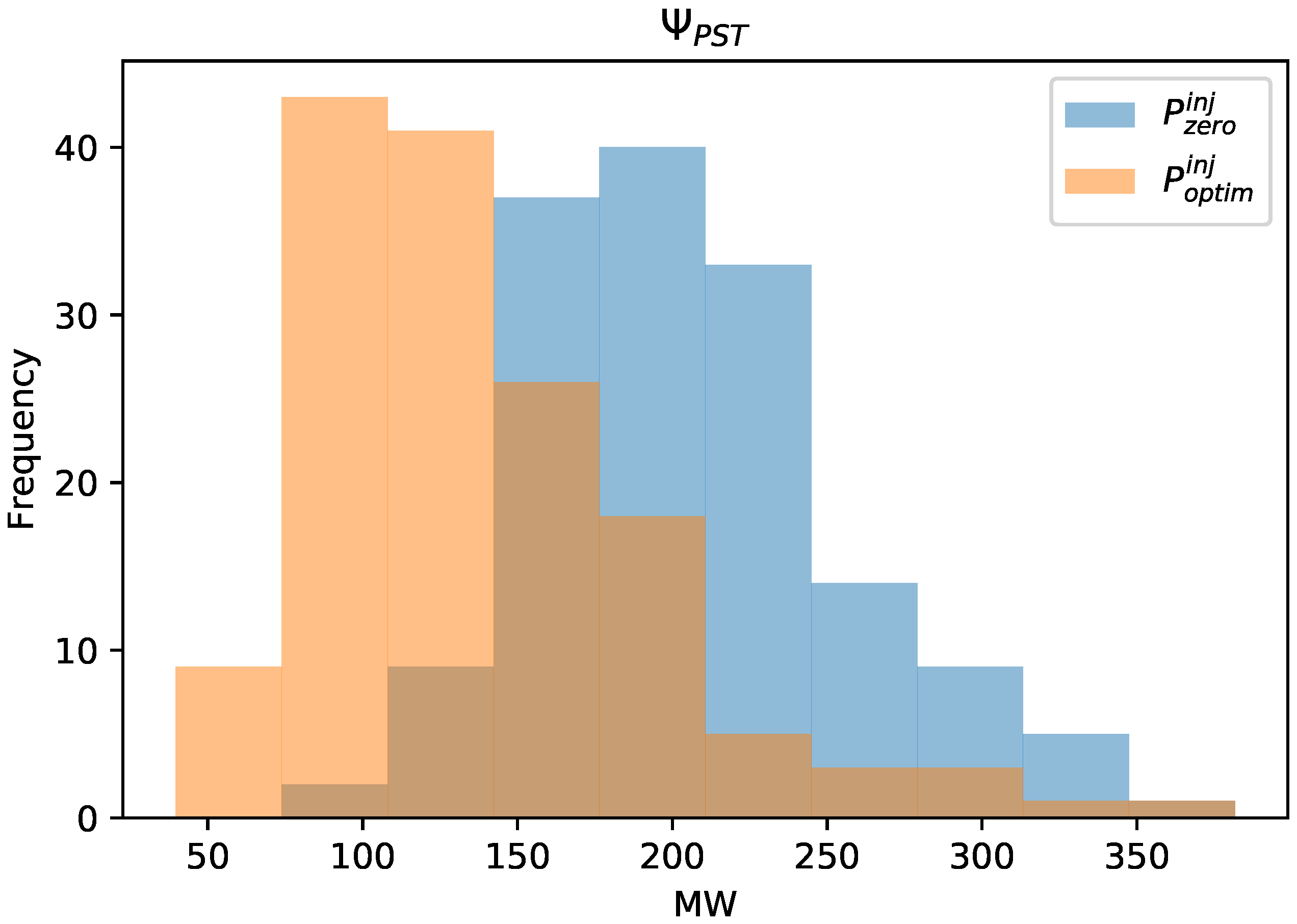
Figure 2 and Figure 3 show the error distribution for the ${\mathsf{\Psi }}_{static}$ and ${\mathsf{\Psi }}_{PST}$ PTDF matrix, respectively, when applying $P_{zero}^{inj}$ and $P_{optim}^{inj}$. Following the same trend observed in Table 6 and

Table 8. Performance indexes for the reduced model, with an explicit PST modeling.

${\mathsf{\Psi }}_{\mathit{static}}$ + $\mathit{PSDF}$	${\mathit{P}}_{\mathit{zero}}^{\mathit{inj}}$	${\mathit{P}}_{\mathit{optim}}^{\mathit{inj}}$
RMSE (MW)	$143.30$	$194.20$
VaR (MW)	$273.10$	$275.30$

, the results demonstrate that, when the operational scenarios with no PSTs modeled ($P_{zero}^{inj}$) were applied to the non PST optimized PTDF matrix (${\mathsf{\Psi }}_{static}$), the errors were lower than when the opposite occurred. With these two figures, the over fitting process that occurred in the optimization process defined in Section 2.2 became clear, therefore, stressing the need for a more general representation of PSTs in the reduced models.

Finally, the reduced model including an explicit modeling of the PST (${\mathsf{\Psi }}_{static}$ + $PSDF$) was tested. For the injected power set where PSTs were optimized ($P_{optim}^{inj}$), the PST of the reduced model mimicked its behavior; in other words, an injected power was multiplied by the $PSDF$ matrix. As presented in Section 2.4, a relationship between degrees of the PST and injected power was established and the same power was injected by the PST in the reduced model.

Table 8 shows the error results for the case where an explicit modeling of the PST was done (${\mathsf{\Psi }}_{static}$ + $PSDF$). As can be observed, for the case where the PST was not optimized ($P_{zero}^{inj}$), the error was the same as presented in Table 6, as the injected power of the PST of the reduced model was set to zero.

When considering the case where the PST was optimized ($P_{optim}^{inj}$), the error showed a slight reduction issue to the explicit PST modeling. In addition, when looking into the VaR, it was observed that, with the explicit modeling, the VaR tended to be similar independently of the considered case.

Figure 4 shows the error distribution for the representation using a PTDF + PSDF matrix. It was observed that the error obtained with the $P_{zero}^{inj}$ was similar to the one presented in Figure 2. For the $P_{optim}^{inj}$, the error was superior to the one obtained with the ${\mathsf{\Psi }}_{PST}$ PTDF matrix (as shown in Figure 3) but inferior to the ones obtained with the ${\mathsf{\Psi }}_{static}$ PTDF matrix.

Comparing both the results obtained with and without the explicit PST modeling, it was observed that relying only on the optimization of the PTDF matrix using a set of data where the PSTs were optimized tended to underperform the case where the PST were not optimized and vice versa. When adding the explicit modeling of the PSTs, the results for the case using $P_{optim}^{inj}$ were not as accurate as the ones obtained with the ${\mathsf{\Psi }}_{PST}$ matrix, but were more accurate for the case where $P_{zero}^{inj}$ was applied.

Overall, the proposed model with an explicit modeling of the PSTs lost some accuracy for a specific case $P_{optim}^{inj}$, but compensated for the opposite case $P_{zero}^{inj}$, as highlighted by the VaR values presented in Table 8.

5. Conclusions

This paper presents a simplified methodology to model PSTs in reduced network models and assesses its effects in transmission networks. The proposed methodology is applied to a real test case allowing to identify challenges that are not easily addressed with simplified test systems. A performance assessment index is proposed that allows assessing the pertinence of representation in a reduced model. Three cases were studied, including the one where no PST representation existed.

Preliminary results tend to show promise for modeling PSTs in reduced network models. The simulations showed that explicitly modeling phase shifters along with the PTDF matrix could increase the level of accuracy of the reduced model compared to the approach based only on the definition of the PTDF matrix. In our view, this highlights the interest of the proposed methodology for the development of reduced static model of a large scale power network, such as the ones performed in [6]. The further deployment of these devices over the network triggers more and more difficulties to a static representation of the power system over its different operation conditions.

It is important to stress that, given the specificities of power systems, results are conditioned by the choice of the simulated PST. A PST in a more central position or next to critical bottlenecks can have a different impact on the system flows and production plan, in the same way as a more decentralized PST can cause the inverse. In addition, it is important to remember that all results were obtained using the DC approximation and should therefore be carefully interpreted as the results of a full AC analysis might differ.

A key direction for further work is to expose the proposed methodology to a larger set of operating conditions, and equipment specificities. It would also be of interest to assess the suitability of such methodology to model HVDC lines and assess its impact on reduced network models.

References

- e–HIGHWAY 2050. D 2.2—European Cluster Model of the Pan-European Transmission Grid; Technical Report; European Commission: Brussels, Belgium, 2014. [Google Scholar]
- Lumbreras, S.; Ramos, A. The new challenges to transmission expansion planning. Survey of recent practice and literature review. Electr. Power Syst. Res. 2016, 134, 19–29. [Google Scholar] [CrossRef]
- Shayesteh, E.; Hobbs, B.F.; Amelin, M. Scenario reduction, network aggregation, and DC linearisation: Which simplifications matter most in operations and planning optimisation? IET Gener. Transm. Distrib. 2016, 10, 2748–2755. [Google Scholar] [CrossRef]
- Wang, L.; Klein, M.; Yirga, S.; Kundur, P. Dynamic reduction of large power systems for stability studies. IEEE Trans. Power Syst. 1997, 12, 889–895. [Google Scholar] [CrossRef]
- Shi, D.; Tylavsky, D. A Novel Bus-Aggregation-Based Structure-Preserving Power System Equivalent. IEEE Trans. Power Syst. 2015, 30, 1977–1986. [Google Scholar] [CrossRef]
- ENTSO-E. 10-Year Network Development Plan; ENTSO-E: Bruxelles, Belgium, 2014. [Google Scholar]
- Marinho, N.; Phulpin, Y.; Folliot, D.; Hennebel, M. Network Reduction Based on Multiple Scenarios. In Proceedings of the 2017 IEEE Manchester PowerTech, Manchester, UK, 18–22 June 2017; pp. 1–6. [Google Scholar]
- ENTSOE–E. Phase Shift Transformers Modelling; Technical Report; ENTSO-E: Bruxelles, Belgium, 2014. [Google Scholar]
- Hertem, D.V. The Use of Power Flow Controlling Devices in the Liberalized Market. Ph.D. Thesis, KU Leuven, Leuven, Belgium, 2009. [Google Scholar]
- ENTSO-E Common Grid Model. Available online: https://www.entsoe.eu/major-projects/common-information-model-cim/cim-for-grid-models-exchange/standards/Pages/default.aspx (accessed on 1 July 2018).
- Ward, J.B. Equivalent Circuits for Power-Flow Studies. Trans. Am. Inst. Electr. Eng. 1949, 68, 373–382. [Google Scholar] [CrossRef]
- Dimo, P. Nodal Analysis of Power Systems; Abacus Bks, Editura Academiei: Bucharest, Romania, 1975. [Google Scholar]
- Lumbreras, S.; Ramos, A.; Olmos, L.; Echavarren, F.; Banez-Chicharro, F.; Rivier, M.; Panciatici, P.; Maeght, J.; Pache, C. Network partition based on critical branches for large-scale transmission expansion planning. In Proceedings of the 2015 IEEE Eindhoven PowerTech, Eindhoven, The Netherlands, 29 June–2 July 2015; pp. 1–6. [Google Scholar] [CrossRef]
- Burstedde, B. From nodal to zonal pricing: A bottom-up approach to the second-best. In Proceedings of the 2012 9th International Conference on the European Energy Market (EEM), Florence, Italy, 10–12 May 2012; pp. 1–8. [Google Scholar] [CrossRef]
- Marinho, N.; Phulpin, Y.; Folliot, D.; Hennebel, M. Redispatch index for assessing bidding zone delineation. IET Gener. Transm. Distrib. 2017, 11, 4248–4255. [Google Scholar] [CrossRef]
- THEMA. Loop Flows–Final Advice; Technical Report; European Comission: Brussels, Belgium, 2013. [Google Scholar]
- Zimmerman, R.D.; Murillo-Sanchez, C.E.; Thomas, R.J. MATPOWER: Steady-State Operations, Planning, and Analysis Tools for Power Systems Research and Education. IEEE Trans. Power Syst. 2011, 26, 12–19. [Google Scholar] [CrossRef]
- ENTSO-E Transparency Platform. Available online: https://transparency.entsoe.eu/ (accessed on 26 May 2018).
- PLATTS World Electric Power Plants Database. Available online: https://www.spglobal.com/platts/en/products-services/electric-power/world-electric-power-plants-database (accessed on 26 May 2018).
Figure 1.
Illustrative example of the performance assessment for a reduction approach.
Figure 2.
Error distribution for the static PTDF matrix representation when applying the and datasets.
Figure 3.
Error distribution for the PST optimized PTDF matrix representation when applying the and datasets.
Figure 4.
Error distribution for the explicit PST representation when applying the and datasets.