Importance of Reliability Criterion in Power System Expansion Planning

1
Croatian Power Company (HEP d.d.), Zagreb 10000, Croatia
2
Energy Institute Hrvoje Požar (EIHP), Zagreb 10000, Croatia
3
Faculty of Electrical Engineering, Computer Science and Information Technology (FERIT), Josip Juraj Strossmayer University of Osijek, Osijek 31000, Croatia
*
Author to whom correspondence should be addressed.
Energies 2019, 12(9), 1714; https://doi.org/10.3390/en12091714
Submission received: 15 March 2019
/
Revised: 29 April 2019
/
Accepted: 30 April 2019
/
Published: 7 May 2019
(This article belongs to the Special Issue Selected Papers from MEDPOWER 2018—the 11th Mediterranean Conference on Power Generation, Transmission, Distribution and Energy Conversion)
Abstract
:The self-sufficiency of a power system is no longer a relevant issue at the electricity market, since day-to-day optimization and security of supply are realized at the regional or the internal electricity market. Research connected to security of supply, i.e., having reliable power capacities to meet demand, has been conducted by transmission system operators. Some of the common parameters of security of supply are loss of load probability (LOLP) and/or loss of load expectation (LOLE), which are calculated by a special algorithm. These parameters are specific for each power system. This work presents the way of calculating LOLP as well as the optimization algorithm of LOLP, which takes into consideration the particularities of the power system. It also presents a difference in the treatment of LOLP regarding the observed power system and the necessary installed power capacity if applied to the calculated LOLP in relation to the optimized LOLP. As a conclusion, the study analyzed the parameters impact the regional electricity market—where the participants are countries with different development levels and various particularities of power systems—i.e., what it means when the same LOLP criterion is applied to them and the optimized LOLP.
1. Introduction
The electricity market and the security of electricity supply are defined by several directives and regulations. One of the most important documents stipulating measures for secure customer security is the 2005/89/EC Directive [1], whereby the energy union concept is based on a few (eight in total) new bills, a new regulation on the preparation for risks being among them, which should replace said 2005/89/EC Directive. The analysis of the adequacy of power systems is conducted by the transmission system operators on the basis of methodological instructions by ENTSO-e, and that report [2] serves as the basis for the assessment of mid-term security of supply of the power system. The basic probability indicators for drawing up the mid-term adequacy of power systems are loss of load probability (LOLP) and loss of load expectation (LOLE). LOLP in a power system is expressed as a percentage of time, annually or monthly, in which the power system will not be able to meet demand with available generation capacities. LOLE is the index on which the basis of LOLP shows the total number of hours in a year, in which the power system will not be able to meet demand. In this paper, reliability calculations are described, followed by examples of generation expansion of a real power system under different reliability indices. As it is stated in [3], it is necessary to quantify the value of lost load (VOLL) to obtain the economic value of adequacy. In order to put a value on reliability, a commonly employed parameter is the VOLL, which measures the damage suffered by consumers when the supply is curtailed. In cases of productive activities (such as industrial processes engaged in the production of a good), an objective measure of the cost of interruptions based on the loss of production or the linked benefit is possible.
At the moment in the European Union (EU), a new Regulation (EU) 2018/2019 of the European parliament and of the Council of risk-preparedness in the electricity sector is being prepared, and repealing Directive 2005/89/EC is supposed to be adopted at the beginning of 2020. As it is described in the new Regulation, the electricity sector in the EU is undergoing a profound transformation, characterized by more decentralized markets with more players, a higher penetration of renewable energy, and better interconnected systems. The main idea of the internal electricity market is that well-functioning markets and systems with adequate electricity interconnections are the best guarantee of security of supply.
A common approach to electricity crisis prevention and management also requires that member states use the same methods and definitions to identify risks relating to the security of supply and are in a position to effectively compare how well they and their neighbors perform in that area. This Regulation identifies two indicators for monitoring the security of electricity supply in the Union—expected energy non-served (EUE), expressed in GWh/year, and LOLE, expressed in hours per year. Those indicators are part of the European resource adequacy assessment carried out by ENTSO-E. In the Regulation, there is a description of the methodology of calculation of security of supply. To ensure the coherence of risk assessments in a manner that builds trust between member states in an electricity crisis, a common approach to identifying risk scenarios is needed. Therefore, after consulting the relevant stakeholders, ENTSO-E should develop and update a common methodology for risk identification in cooperation with the Agency for the Cooperation of Energy Regulators (ACER) and with the Electricity Coordination Group (ECG), which was set up by a Commission decision on 15 November 2012 as a forum in which to exchange information and foster cooperation among member states—in particular, in the area of security of supply—in its formation composed only of representatives of the member states. ENTSO-E should propose the methodology, and ACER should approve it. When consulting the ECG, ACER is to take utmost account of its views. ENTSO-E should update the common methodology for risk identification where significant new information becomes available.
ENTSO-e conducts studies about Scenario Outlook and Adequacy Forecast, trying to calculate a Pan-European power system adequacy. In their report [2], there is a question raised related to capacity adequacy. If the reliability index is met beyond the national legal requirement, how large is the related capacity margin surplus available for the neighboring area, or even system wide? Additionally, if the reliability index is not met, by how much would the available capacity need to increase to meet the target? Another question is about the methodology applied.
The LOLP index is used in the analyses of generation parts of power systems but also in reliability analyses of both the transmission and the distribution system. There are many more papers regarding the use of VOLL for both transmission and distribution system analysis. VOLL is an essential parameter for transmission system reliability management [4]. Theoretical analysis shows that using more detailed VOLL data allows for better-informed transmission reliability decisions. Incorporating variations and uncertainties into expansion planning produces a plan that has better economy and reliability performance during operations. Recent progress on robust optimization techniques can consider uncertain parameters in expansion optimization [5].
There are also some papers and studies regarding planning a reserve margin, which is a common metric used in generation planning to determine an electric utility’s resource need above the typical annual peak load. As a proxy for system reliability, the planning reserve margin is useful in informing resource decisions between detailed reliability studies [6]. Questions about providing electricity with adequate power quality and reliability at a reasonable rate are becoming more important. Therefore, there are a number of country-specific analyses, such as German security of supply or questions about capacity market [7,8]. Of high interest in the field of reliability of power systems or the security of supply is a capacity market or remuneration mechanism. In Reference [9], the analysis begins with identifying the optimum level of investments to the 2030 horizon to ensure capacity adequacy, assuming a reference scenario of EU energy system developments, followed by a simulation of the operation of a wholesale energy-only market to estimate the ability of these investments in order to recover their capital cost. The amount of capacity remuneration required to cover for the missing revenue margin is estimated, as are the implications from hypothetical asymmetric remuneration across the member-states of the EU. Also in Reference [10], there is a question raised regarding the competitive energy market and whether it will be sufficiently addressed in the capacity market to garner adequate resources to keep the lights on. The European electricity market has been constructed as an “energy only market” without the compensation for the costs of generation adequacy. Such a market is able to operate in the presence of the capacity excess. However, gradually, the power reserve margins have been diminishing, causing a fear of power balancing in the coming years [11]. All those papers are dealing with one common question—security of supply or capacity adequacy? The basic methodology always relies on a probabilistic approach.
The consequence of capacity shortage is the reduction in electricity supply, which results in a certain VOLL or energy for customers. The reserve of a power system in all three technological parts—generation, transmission, and distribution—depend on the level of damage, i.e., the specific level of value of undelivered kWh of electricity. Both LOLP and LOLE indices are calculated via an algorithm in which the equivalent curve of load duration is formed by the method of convolution [3,4,5,6] from the load duration curve, taking into consideration the probability of outage of every individual generation facility as well as the outage cost, which is VOLL times unserved energy. The fundamental thesis in this paper states that LOLP, and thus LOLE, should not be calculated, but may be optimized regarding VOLL and the available technologies for new generation facilities. The paper further analyzes power systems with different optimum levels of LOLP, which participate in the electricity market. The main objective of this paper is to better understand reliability by the optimization of LOLP and LOLE regarding VOLL and available technologies for new generation facilities.
2. LOLP Optimization Methodology Description
Computer models for the analysis and the planning of the power system were developed on algorithms that described certain aspects of power systems; some of them were simulations, some were optimization types, and some models were a combination of the two [12,13,14]. One of the most famous models used to calculate the LOLP through long-term planning of a power system is the Wien automatic system planning package (WASP), which is used in this analysis as well. The basis of such analysis is load duration curve (LDC) of the power system. When taking into consideration the probability of the first unit outage, the result is the equivalent load duration curve (ELDC1). The result of the outage of two first units is ELDC2, and ELDCn is the result when the probability of the outage of the last unit is taken into consideration [13,15]:
where ELDCn is the equivalent load duration curve after unit n is on the grid; p is the probability that unit n is available; q is the probability that unit n is unavailable; MWn is the capacity of unit n and x is load. The expected generation for each unit is then:
where En is the generation of unit n; T is the time period represented by the load duration curve; ELDCn−1 is the equivalent duration curve, which incorporates the effect of the force outages of unit n−1; an is the system capacity for units 1, 2, 3,…, n−1; and bn is the system capacity for units 1, 2, 3,…, n.
For certain installed capacities of all power plants in the power system (ICP), LOLP is the index determining the probability of the occurrence that the load is higher than the sum of the available capacities of all considered power plants. Energy not served (ENS) is electricity that will not be delivered and represents a part below the ELDCN curve limited by ICP on the left side, as it is shown in Figure 1.
To complete the calculation of LOLP, it is necessary to calculate the total cost of the power system, as described in [13,14]. The optimization of the total cost of the power system requires the minimum of a goal function in a specific scenario of the development of the power system. The objective function represents the total cost of the power system, which consists of investment costs for new power plants, fuel costs, operation and maintenance costs (O & M), costs of VOLL, and the remaining value of new power plants after the last planning period year. The LOLP and the LOLE indices are calculated for each year.
B represents the total cost of the power system of the observed scenario; I is the capital investment cost in new generation units; S is the salvage value of investment costs after the last year of the observed period; F represents the fuel costs; M represents the non-fuel operation and the maintenance costs; VOLL is the outage costs; t represents the years of the scenario; T is the length of the study period, i.e., the number of years in the scenario; and index j is the observed scenario of the generation expansion.
Three main LOLP optimization steps are described as follows:
- In the first step, one should calculate the power capacity to meet LOLP criteria from 5% to 0.001% on a technical level without any economic consideration. Those values are taken from expert analysis as very high and low boundaries of the LOLP value. The results of calculation for each value of LOLP (starting from five and ending with 0.001%) are the number of MW of installed capacity that should be built in order to meet the criteria of LOLP. Those calculations are conducted under no economical limitations. Thus, the first step is a calculation of how many MW’s have to be installed to meet the reliability criteria of LOLP values. That is why LOLP values are first calculated for various combinations of operating power plants. The key point in this stage is to consider reliability aspects only, which means that economic variables are excluded. LOLP criterion is met by introducing new power plants only when it is necessary to satisfy the reliability criteria regardless of the costs of the power system. The solution is acceptable if the calculated LOLP value is lower or equal to the proposed one for all years of the planned period, i.e.:where LOLPUL is the proposed value of LOLP for which the new construction of power plants in the power system is calculated. One can analyze the impact of different technologies or different characteristics of the same technologies of new generation capacity in order to conduct sensitivity analysis.
- The second step considers economic variables for each value of LOLP or the calculated combination of the necessary power plant capacity for a specific value of LOLP from 5% to 0.001%. In this second step, the objective function B (total cost of the power system) is a function for comparison of different scenarios. It takes into consideration the investment of new capacity, O & M cost, fuel cost, outage cost, salvage value, etc.
- The third step or case study considers different combinations of power plant capacity for different values of LOLP on a model of a power system. In this paper, it is a Croatian power system, which was taken as a real model. There are four scenarios modeled and compared, two of them with limited LOLP and two of them with no limitation of LOLP.
3. LOLP Optimizing Case Study Analysis
In this paper, two technologies were chosen for power plant candidates—a coal-fired thermal power plant and a natural gas-fired combined gas power plant with usual characteristics taken from literature. Analyses were conducted separately for power plant candidates, coal-fired thermal power plants (TPP), and natural gas-fired combined cycle gas turbine power plants (CCGT). The values of LOLP were simulated for this analysis ranging from 5% to 0.001%. Results are shown in Figure 2.
It should be noted that new generation capacity was added in quantities of 20 MW in order to have smooth or continual curves. Characteristics of such small units are the same as regular size units in both analyzed technologies.
After calculating the necessary new constructions of power plants with the given value of LOLP for each LOLP limitation separately, the objective function was calculated for two levels of VOLL—$2 USD/kWh and $10 USD/kWh.
Two levels of VOLL were chosen for analysis, one of $2 USD/kWh and the other of $10 USD/kWh. The former correlated with the gross domestic product (GDP) of around $10,000 USD per capita, and the latter with the GDP of around $40,000 USD per capita [16,17,18]. The aim was to compare two different levels of economic systems—a developing one and a developed one. It was estimated that there was no need to consider more levels of outage, since this analysis showed differences between higher and lower levels of outage, which corresponded to different developments of economic systems. Other data referring to specific costs of fuel and maintenance were taken from [19,20].
Optimizing the analysis of LOLP started with the calculation of necessary installed power in the observed power system under the limitation of LOLP of 0.0001% (0.5 minutes per year), 0.001% (5.5 min per year), 0.01% (52 min per year), 0.03% (2.5 h per year), 0.05% (4.5 h per year), 0.07% (6 h per year), 0.1% (9 h per year), 1% (3.6 days per year) and 5% (18 days per year) with two levels of outage of $10 USD/kWh and $2 USD/kWh. It should be noted that the same power system was always analyzed, and limitations of LOLP varied just as with VOLL. After obtaining the combination of existing and new power plants, i.e., the total available power for each respective year and for each observed LOLP, the costs of the power system, i.e., the goal function, was calculated as described in the previous chapter. All the values calculated in the goal function refer to the year 2018, which was used as the base in this analysis.
If LOLP was limited at 0.0001%, which is an extreme requirement (usual value amounts at 8 h or 0.1%, e.g., in Ireland), there was a visible increase of necessary capacity or investment costs related to constructing new generation capacities, which was understandable considering the high demand of reliability of the power system. Such a level of security of supply could not be considered necessary due to questionable economic profitability, since the power system disposed a very large reserve (if isolated), thus such a power system would be considered over-capacitated in a techno-economic sense. If such a power system was observed in reality, necessary construction for fulfilling a certain safety level of supply, e.g., of 0.0001%, there would be a need to ensure huge amounts of generation capacities reserve if there were a consideration of not being in the regional electricity market. Where these capacities would be placed in a mathematical sense is not of much importance, except for the fact that they would need to be available, i.e., properly electrically connected.
When the necessary construction of generation capacities of a power system with a coal-fired thermal power plant was analyzed depending on the level of LOLP, we got a curve of necessary construction, as shown in the Figure 3. This curve of necessary construction of generation facilities depending on the LOLP fit well with the theoretical curve. The probabilities (which were extremely small) for which the limitation of LOLP was very small (<0.001), necessary construction of generation capacities grew asymptotically by coming closer to the ordinate axe.
If a certain value is added to unsupplied kWh of electricity, then the outage cost becomes dominant in the goal function of the total cost. As a result, the total costs of the power system grow as the level of security of supply decreases. However, more power plant construction leads to a level of higher security of supply. In this case, as more power plant capacities demanded higher investment, the dominant member of the goal function referred to the investment into new power plant capacities, thus the total cost of the power system grew. Therefore, the goal function of the total cost regarding different values of LOLP had the form of a bathtub curve with one more or less expressed as the minimum.
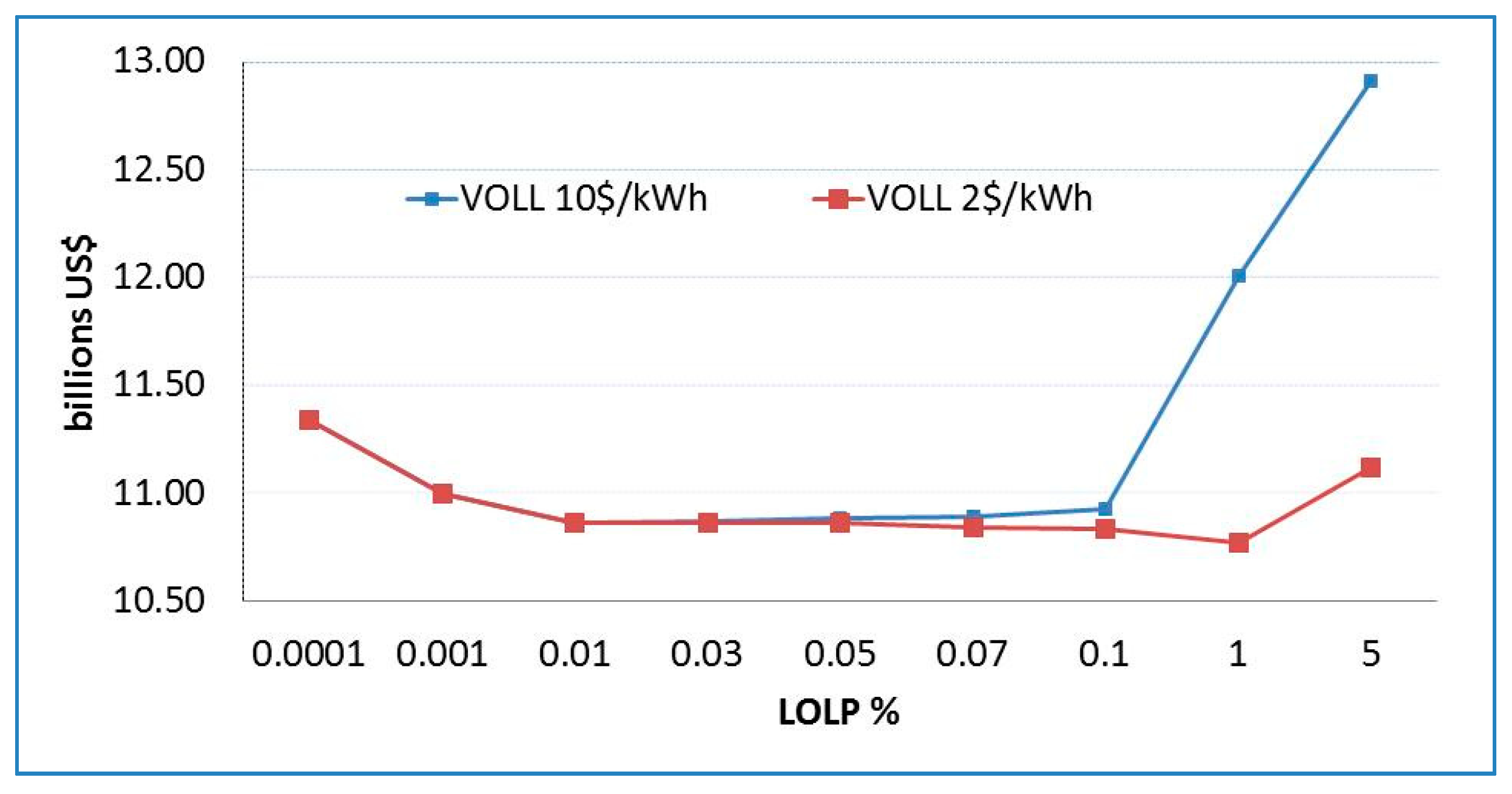
In the cost structure of the power system, it is visible that investment costs, residual value, and fuel costs were the same in both observed cases for VOLL of $2 USD/kWh and $10 USD/kWh starting from LOLP 0.01%, which was understandable since investments for necessary new construction of power plants depended on the given security of supply, and fuel consumption depended on electricity consumption. In the case of VOLL of $10 USD/kWh, the total outage cost as the component of the total cost of the power system increased sharply. It was expected that, in the case of a LOLP value higher than 5%, they would eventually become a dominant part of the total cost of the power system.
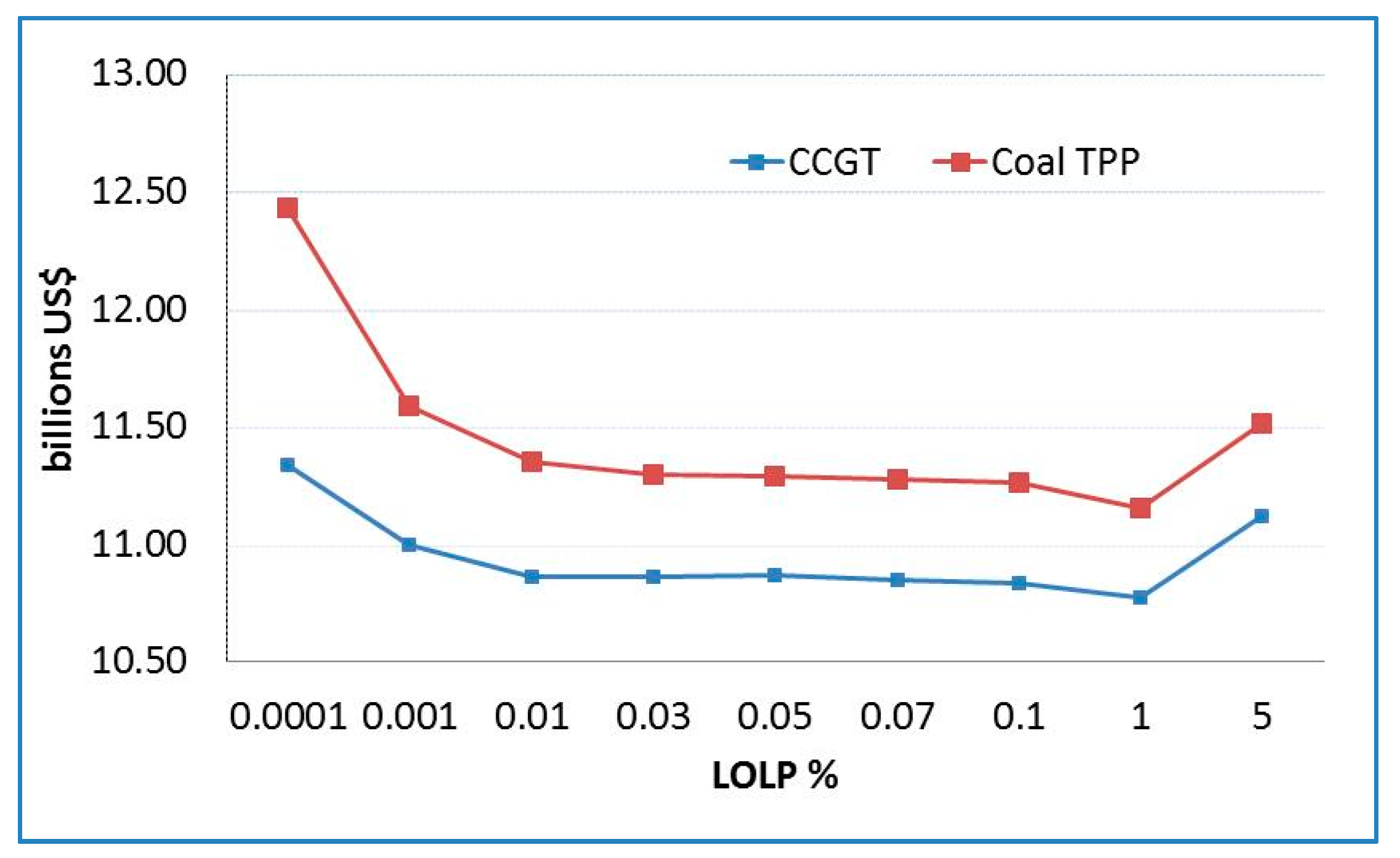
These costs were added and presented according to VOLL of $2 USD/kWh and $10 USD/kWh, and the curves of the total costs were obtained. The change of total costs depending on the security of supply in the case of the combined cycle gas turbine (CCGT) only was milder than the case with the coal-fired power plant only. The reasons for this were primarily lower investment costs of new power plants and a lower probability of power plant outages, as shown in Figure 4.
LOLP would accordingly be some kind of necessity or signal for the construction of the power system. In this example, it would particularly refer to the generation capacity, which needed to fit the economic condition of the country, i.e., the power system being analyzed. Optimum LOLP represents not only the criterion for the necessary construction of power plants (i.e., generation capacity) but also an analytic parameter that shows the level of development of the power system and the economic condition as well, i.e., the standard of living of its inhabitants, usually described as GDP per capita. The variable that describes the level of development particularly well is VOLL, and the variable is shown as the one that can connect the level of construction of the power system and the level of economic development. Of course, it is expected that the power system is better constructed, i.e., that more generation facilities are constructed if economic activity is more intensive, i.e., if an economic system can generate a level of additional value that may construct and maintain such a power system to fulfill customers’ needs in critical periods. However, if the economic system is not well developed and cannot generate additional value to invest into the energy sector, the power system is then weaker, especially in terms of generation. Consequently, the transmission part of the power system is shown as less reliable and less constructed. On the other hand, electricity and reserve in the power system can be bought at the electricity market. In any case, the construction of generation facilities or the procurement of such facilities, i.e., of electricity at the electricity market, requires additional financial means. An economy that is developed and that has a big additional value is expected to be able to ensure electricity at a considerably higher price in critical periods. The question is whether there will be enough available capacities, which presents a risk. This risk is best described as a dependence on generation facilities, whose work cannot be controlled; without those facilities, there is no safety, long-term or short-term, regarding electricity procurement, amount, dynamics, and quality.
If necessary, power plant construction is a function of LOLP, one gets curves of necessary power, as shown in Figure 5. These curves fit well with theoretical curves of necessary new construction of generation facilities depending on security of supply. In part of the curve with LOLP, from 0.0001% to 0.003%, the difference in necessary construction totals equaled hundreds of MW, as seen in Figure 2. The curve of necessary new construction for the case of the coal-fired TPP showed more value because of less reliability of such facilities in comparison to the gas-fired CCGT. Those differences became negligible for LOLP values higher than one and lower than 0.1 percent.
The final (third step) in the determination of the optimal security of supply in comparison to the outage cost was derived by comparing the total costs of the power system for both observed levels of the outage cost. Analysis was carried out with two technologies, the coal-fired TPP and the CCGT.
Figure 5 and Figure 6 show the total costs of the power systems for both observed technologies of the coal-fired TPP and the CCGT depending on the security of supply for the level of VOLL of $2 USD/kWh and $10 USD/kWh. The differences in total costs for the different technologies were expressed at higher levels of customer security of supply, i.e., at lower levels of LOLP when a much higher installed capacity of new power plants was necessary.
Apart from specific characteristics of the analyzed power plant, it is important to see that the VOLL changed the form of the total power system costs curve. For lower levels of VOLL (e.g., for $2 USD/kWh) the diagram of the total cost of the power system is rather symmetrical, while in case of higher VOLL (e.g., for $10 USD/kWh), the curve of total costs clearly expressed minimum.
In conclusion, qualitative analysis of a power system requires the knowledge of economic development levels as well as its perspective. The measure of economic development, which as a variable influences the necessary construction of the power system, is the VOLL. Therefore, we should emphasize that economic development is not the only variable influencing the development of the power system, but it is definitely one of the key variables influencing inhabitants’ living standards, traffic intensity, etc. A developed economy enables the development of a power system. Therefore, this is a firm connection between energy, power, and an economic system. The better developed those systems are, i.e., the more synchronized the development of the economic and the power systems is, the narrower the area of optimum construction, i.e., the minimum of total costs, will be.
Interconnected power systems (electrically, regulatory, and economically, which is defined by the electricity market) may count on the power and the energy procured on the market, not only in the case of trading but also in day-to-day operations as a result of operational costs optimization [21,22,23]. As opposed to self-sufficient power systems in the case of the regional electricity market, the LOLP is not the result but is set as a criterion. Thus, in that case, we may talk about risks managing the possibilities of procuring losses and delivering surpluses. If there are no possibilities of procuring power and energy at the market, and the power system is not developed enough, the LOLP increases and goes into the right part of the diagram, as shown in Figure 5 and Figure 6. In those cases, not only does the procurement of power and energy at the market become important, but the price becomes important as well, which grows due to increased demand in critical periods. Consequently, there is an increase in the total costs of the power systems. Which marginal price of power and electricity is economical or possible to procure power and energy at the market depends on the possibilities of purchase and sale, the economic system development, the available generation capacities, the electricity prices in the regional market, etc. Generally, the more developed and the richer an economic system is, the higher price it can take (Italy, for instance), and vice versa. According to this, the LOLP index expresses the measure of constructiveness of the observed power system, the availability of the generation facilities in the surroundings, and the price of electricity present with the risk of procurement from the market.
Furthermore, in the case of over-construction (installation) of generation facilities in the power system, we arrive to the left part of the diagram, as shown in Figure 5 and Figure 6. These figures display the state of over-construction of the power system if only the observed power system is taken into consideration. Of course, this is just a partially correct view, since power plants (in most cases) are not built to supply one power system but to generate electricity and sell it to customers or to the regional market. The investors build power plants where the final price of electricity is higher, competitive at the market, and where they can sell electricity to customers. However, from the point of view of national energy safety, customer security of supply is higher if the power system is over-constructed, i.e., if there is enough constructed power plants, generation, and other energy facilities, regardless of equivalent working hours. The diagram shows that the minimum of the curve of total costs of the power system moved to the left. The curve’s gradient of increase of total costs of the power system for the cases of lower safety levels of customer supply was higher, which means that the increase of total costs due to increase of total damage due to undelivered electricity was more intensive. In practice, this does not mean that power system that has capacity adequacy at its disposal would suffer from reductions. Namely, it is necessary to settle necessary power and energy from neighboring power systems, i.e., at the market of electricity, under the condition that it is available in the amount and the dynamics, such as the price necessary to settle the electricity consumption of the observed power system. In such circumstances, the power system is oriented towards the import of electricity.
4. Case Study
In this analysis, there are four scenarios, as follows:
- −
- SC_0.01% $10—in this scenario, LOLP was limited at 0.01%, VOLL was taken at the level of $10 USD/kWh,
- −
- SC_1% $2—in this scenario, LOLP was limited at 1%, VOLL was taken at the level of $2 USD/kWh,
- −
- SC_LCP $10—in this scenario, LOLP was not limited, the amount of reserve capacity was calculated by the least cost planning (LCP) algorithm, and VOLL was taken at the level $10 USD/kWh,
- −
- SC_LCP $2—in this scenario, LOLP was not limited, the amount of reserve capacity was calculated by the least cost planning algorithm, and VOLL was taken at the level $2 USD/kWh.
All four scenarios presumed the same level and characteristics of electricity consumption and the same characteristics of the new power plants.
Since the field of interest for analysis is defined by values for which the total observed costs are at a minimum, this chapter analyzes the case study scenario of power system development for LOLP values in the field from 1% for the scenario of VOLL of $2 USD/kWh to 0.01% for the scenario of VOLL of $10 USD/kWh. In addition, scenarios of a limited value of LOLP are analyzed. The comparison of these scenarios indicates the essence of the differences between the concepts of the generation expansion planning.
The main results in every scenario presented the number of power plants or the total new capacity becoming operational in the observed period. Although putting power plants into operation was different for each observed scenario, a certain measure of available generation capacity for each scenario was presented by the total construction of the power plants at the end of the observed period necessary to meet certain LOLP requirements. The number of each thermal power plant candidate in a certain year was defined by the number of units that became operational that year.
Load factor of thermal power plants is generally a good indicator of power plant utilization in the power system. Load factors of new power plants, i.e., candidate power plants, were analyzed and aggregated according to technology. Due to the fact that exchange with neighboring power systems was not modeled, the presumption in the analysis was that electricity generation in the thermal and the hydro power plants met the demand. This, of course, meant that the electricity generation was reduced just to meet demand, but it also showed the relation between the necessary generation capacity increases to meet LOLP criteria. Obviously, there was a need for the power plant to work as long as possible to ensure return of investments.
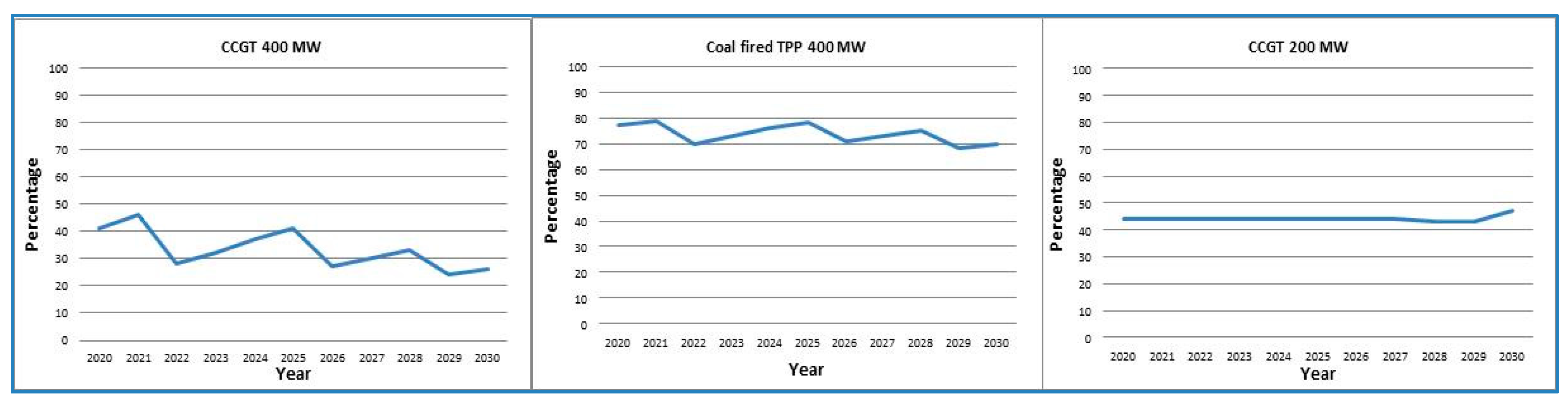
Figure 7 shows the load factor curves of three new thermal power plants, which were analyzed in a scenario with LCP and VOLL of $10 USD/kWh as new thermal power plants, and as such, were put into operation in various years of observed periods.
The left diagram on Figure 7 shows the load factor of the CCGT. The load factor varied regarding other power plants being put in the operation, e.g., the coal-fired TPP. In comparison with the coal-fired TPP, the CCGT had lower investment costs and significantly higher fuel costs, thus the power plant had a lower priority in engagement, and its generation depended on the existing structure of generation in the power system.
As opposed to the 400 MW CCGT, the coal-fired TPP had an even load factor over the years, primarily due to the fact that it had a strong priority in engagement to cover load diagram because of the variable cost of electricity production, e.g., fuel prices. As a case study, the CCGT of 200 MW was set to the same techno-economical characteristic as the one of 400 MW apart from its installed power and technical minimum. It was shown that the load factor for that thermal power plant was even because it was the thermal power plant of lower capacity, thus its relative oscillations of total generation were lower than with a combined gas-fired thermal power plant of 400 MW.
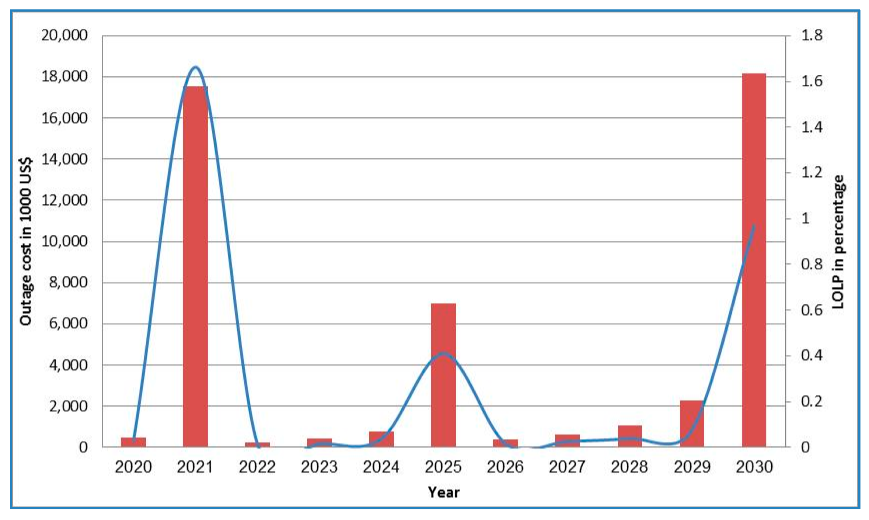
This scenario was characterized by a LOLP diagram and a diagram of outage cost per years, as seen in Figure 8. Outage cost (OC) is a kind of damage suffered by consumers (industrial, service, households, etc.) when the supply is curtailed because the power system is not able to meet demand. Outage cost is the total cost, and VOLL is the specific cost, usually expressed in currency over kWh of electricity not delivered to customers. In our study, the first third of the observed period was significant, since the existing state of construction of the generation facilities was adequate to fulfill the security of supply criteria. The maximum value LOLP reached was 0.63% in the years after decommissioning the power plants that were operational in the planned period.
In the scenario in which LOLP was given at the level of 0.01%, putting power plants into operation was somehow different, just as the total construction at the end of the observed period was different.
Load factors of new power plants had a decreased gradient towards the end of the observed period. This was understandable if we consider that more power plants were put into operation due to increased levels of customer security of supply along with the similar electricity consumption. This meant that, in this construction scenario, it was a priority to engage power, as seen in Figure 9.
The curve of the value of LOLP and the outage cost per year in the observed planned period showed significant variations, but remained within the framework given by limiting the value to 0.01%. Of course, oscillations depended on putting new power plants into operation and thereby a much higher necessary installed power. All the curves are shown in Figure 10.
The next group of scenarios was analyzed with the VOLL $2 USD/kWh for two cases, one without limiting the value of LOLP and one limiting the value of LOLP onto 1%. Load factors of power plant candidates remained almost the same on average, but the load factor of the 400 MW CCGT varied depending on the new thermal power plants put into operation, especially the coal-fired TPP. All the curves are shown in Figure 11.
The curves in Figure 12 convey the value of LOLP and the outage cost per year, which showed characteristic behaviors. One of those was year 2022, the fourth year when no TPPs were put into operation. The maximum achieved value of LOLP was 3.95%.
Load factors of new thermal power plants, especially the coal-fired TPP and the 200 MW CCGT, which were put into operation in the observed period, were relatively constant, whereby the load factor of the CCGT with higher capacity slightly decreased towards the end of the planned period, as seen in Figure 13.
The curves of the outage cost as well as the values of LOLP per year are presented in Figure 14. Characteristic years for this group of scenarios were 2021 and 2025 as well as the last year of the planned period.
5. Scenarios Comparison
The comparison of these four scenarios was possible based on three elements. The first comparison was of scenarios in the group with the same level of VOLL for two different levels of LOLP. The second comparison of scenarios was on the basis of the same level of LOLP for two levels of the VOLL. The third comparison was for different levels of VOLL and LOLP.
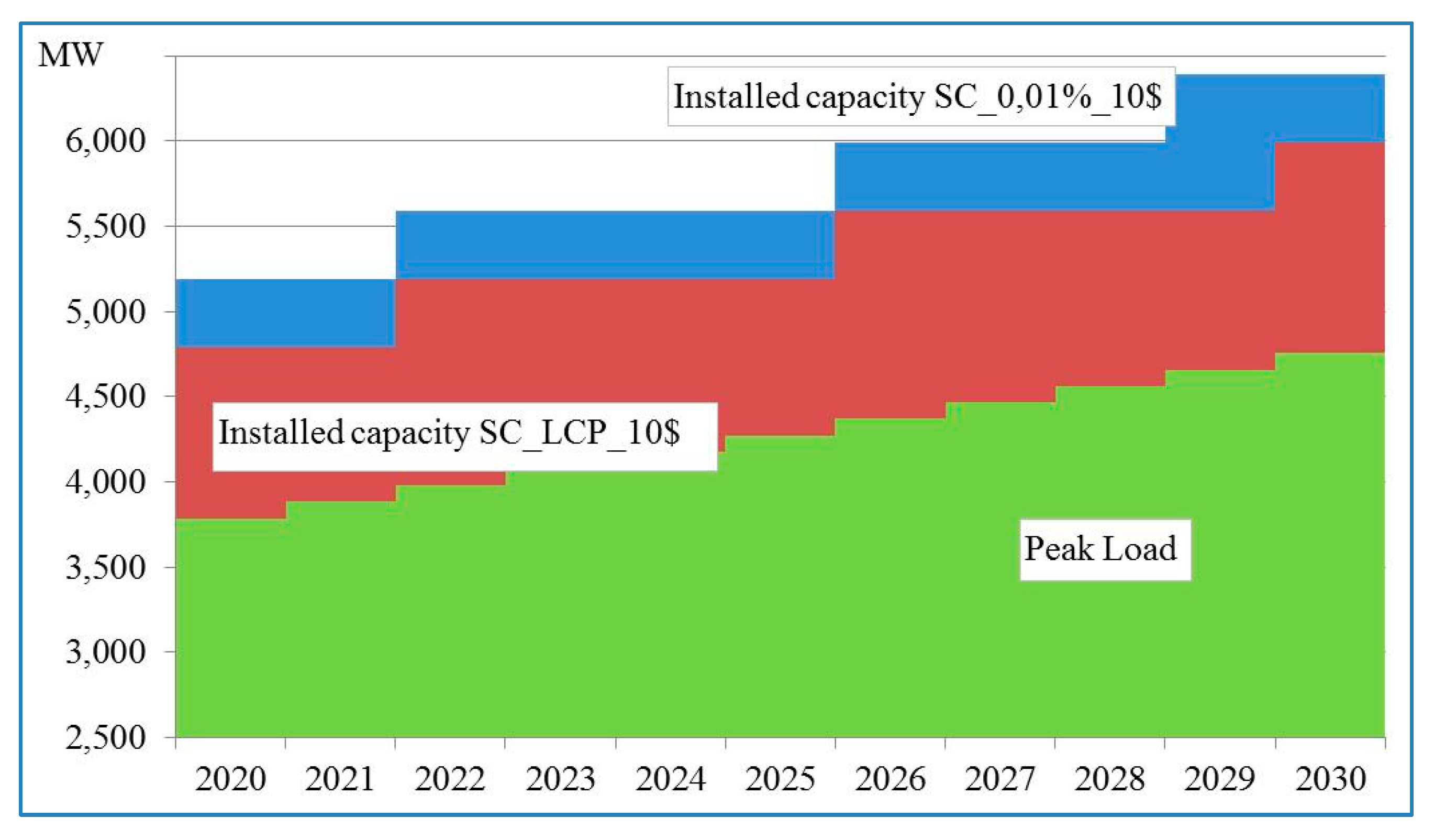
The comparison of scenarios with VOLL $10 USD/kWh and for LOLP of 0.01% without limitations showed significant differences in the second half of the observed period. If the scenarios were compared according to total installed power or the necessary new installed capacity, as shown in Figure 15, it was obvious that by 2019, the installed total power was almost the same, i.e., the necessary new installed capacity. As previously stated, the scenario without limitations corresponded to the LCP scenario, whereas the second scenario with LOLP 0.01% was the scenario with the optimized level of LOLP.
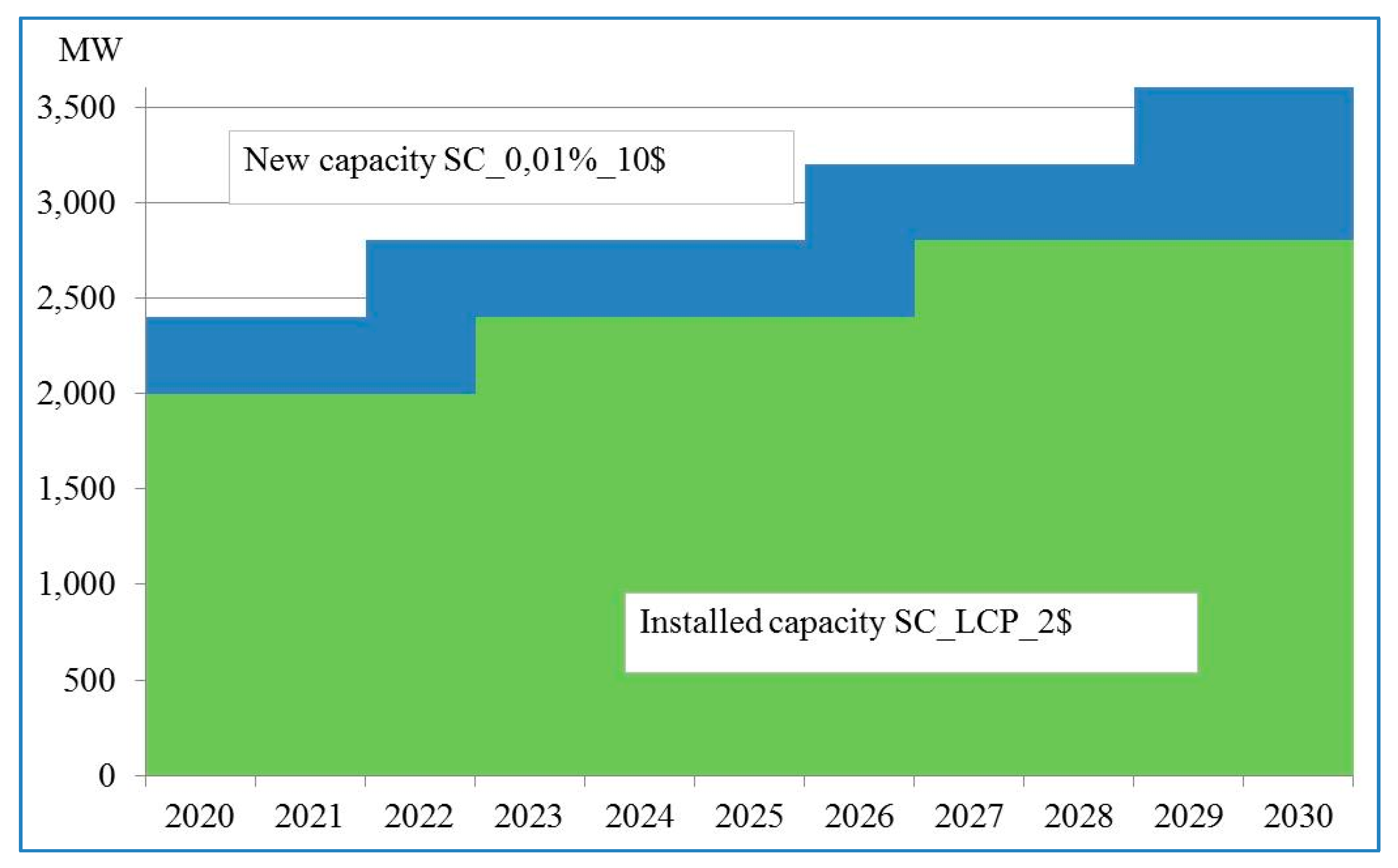
The comparison of scenarios with VOLL $2 USD/kWh and two levels of LOLP without limitations and with a limitation of 1% is shown in Figure 16. These two scenarios differed only in the dynamics of necessary realization in two years of the observed period. This was seen in the second half of the planned period in a way that one power plant was the candidate in the scenario with LOLP of $2 USD/kWh and was put into operation a year earlier than in the scenario without the limitation of LOLP. That meant that, in the group of scenarios with low outage costs, there was actually no difference between generation expansion planning using the method of LCP and the method of optimizing LOLP. The reason for this was that the influence or the share of costs referring to outage cost was almost negligible. These costs went from 0.3% for the scenario with LOLP 3% to 0.96% for the scenario without limitations of LOLP.
This would mean that the issue of customer security of supply for low levels of GDP was not relevant. That issue becomes relevant with the development of an economy and therefore the increase in total GDP, i.e., GDP per capita.
The comparison of two scenarios—in this case, the scenario with VOLL $2 USD/kWh and the level of LOLP without limitations compared to the scenario with VOLL $10 USD/kWh and the level of LOLP of 0.01%—regarding the necessary new construction of power plants is shown in Figure 16.
In this example, there were quantified differences between the necessary constructions of the generation facilities for the LCP scenario compared to the optimized level of the LOLP scenario. The conclusion was drawn that, for a developed economy measured by the VOLL $10 USD/kWh, it was necessary to dispose of the capacity in power plants higher than 400 to 800 MW. It should be noted that additional installed generation capacity was not necessary because, in both scenarios, it was modeled in the same way. However, it was necessary for fulfilling the criteria of customer security of supply. Namely, a high level of economic development consequently had a high level of outage cost, which then in turn necessitated a high level of customer security of supply, requiring additional necessary installed capacity for an equal level of electricity consumption. The difference between these two scenarios was critical. The first scenario corresponded to the method of LCP of the power system, whereby the second corresponded to the scenario with given criterion of LOLP, i.e., directly to the set level of customer security of supply. Apart from that, the difference was in the level of VOLL.
Figure 17 shows the comparison of the necessary new construction of generation capacities for the scenarios corresponding to the LCP scenario for VOLL $2 USD/kWh and $10 USD/kWh. The differences arose from the contribution of outage cost.
6. Conclusions
This paper presented a developed method for incorporating reliability criterion in the optimization of power system expansion planning. Analysis of security of supply was significant when power systems were poorly interconnected with other power systems, which is once again significant when considering the regional electricity market as a real business environment.
The basic measure of security of supply is the reserve capacity in the power system. The better developed an economy is, the more justified a bigger reserve capacity is because of a higher value of VOLL, and vice versa. This means that security of supply is an economic category with a different value in economies on different levels of development. The optimal level of LOLP differs for different levels of VOLL as well as analyzed technology of new power plants, and this was clearly presented in the paper. It was shown that LOLP should be calculated rather than proposed as a pre-specified value, since LOLP depends on VOLL, which is a certain measure of economic development and is changing through time in undeveloped economies. The key variable defining the necessary reserve capacity in a power system is VOLL, whereas in developed economies, the key variable is LOLP. Therefore, LOLP has a different meaning in different circumstances. In the case of LCP, LOLP is an economic parameter, and in the case of optimizing, LOLP is a technical parameter.
Self-sufficiency of a power system cannot be economically justified, since in the case of a big reserve capacity, the load factor of power plants decreases, thus the economics of such power plants are questionable. Power systems with a big reserve capacity need a regional electricity market to improve the economics of such power plants. Therefore, it is reasonable to expect that electricity generation capacities would be economical if they were on an electricity market, which would have a favorable influence on the price of electricity at the market. As was shown in the paper, load factor decreases in the case of a small value of LOLP, and this is not acceptable from an economical point of view.
One should note that electricity trade between developed and undeveloped countries would put undeveloped countries at a disadvantage. The reason lies in the fact that developed countries will have the economic power to construct enough (or more) generation capacities for the appropriate LOLP, whereby undeveloped countries will not be able to do so, since a significantly lower LOLP is optimal for them. LOLP as main criteria for security of supply depends on VOLL, and characteristics of power plants technology are changing over time. The main conclusion of the paper is that, for generation expansion planning on the electricity market, the least acceptable LOLP rather than the LCP should be a criterion for the necessary constructions in a power system; this paper particularly referred to the generation capacity needed to fit the economic condition of the considered country and its power system.
Author Contributions
Conceptualization, Formal Analysis, Writing—Original Draft Preparation, G.S., Methodology and Validation, M.Z., Supervision, Writing-Review & Editing D.Š.
Funding
This research received no external funding.
Conflicts of Interest
The authors declare no conflict of interest.
References
- Directive 2005/89/EC of the European Parliament and of the Council. 2006. Available online: https://eur-lex.europa.eu/legal-content/EN/TXT/PDF/?uri=CELEX:32005L0089&rid=7 (accessed on 15 March 2019).
- ENTSO-e Target Methodology for Adequacy Assessment, October 2014. Available online: https://docstore.entsoe.eu/Documents/SDC%20documents/SOAF/ENTSO-E_Target_Methodology_for_Adequacy_Assessment.pdf (accessed on 15 March 2019).
- Identification of Appropriate Generation and System Adequacy Standards for the Internal Electricity Market, European Commission, Directorate-General for Energy, Directorate B—Internal Energy Market, Unit B2—Wholesale markets; electricity & gas, Brussels. 2016. Available online: https://ec.europa.eu/energy/sites/ener/files/documents/Generation%20adequacy%20Final%20Report_for%20publication.pdf (accessed on 15 March 2019).
- Ovaere, M.; Heylen, E.; Proost, S.; Deconinck, G.; Van Hertem, D. How detailed value of lost load data impact power system reliability decisions - a trade-off between efficiency and equity, SSRN Electronic Journal, January 2016. Available online: https://poseidon01.ssrn.com/delivery.php?ID=565072116003087011122004124023073067058053071002044010118007113106095012108104116070110021048011118001020023030069113027022000118026088041040106015004030068103064003040085110000092008096096072065100011067099027122121080125000116122112082079083001077&EXT=pdf (accessed on 15 March 2019).
- Electric Grid Expansion Planning with High Levels of Variable Geberation, Oak Ridge Laboratory, February 2016. Available online: https://info.ornl.gov/sites/publications/files/Pub59037.pdf (accessed on 15 March 2019).
- Estimating the Economically Optimal Planning Reserve Margin, Energy and Environmental Economics, Inc., USA. 2015. Available online: https://www.epelectric.com/files/html/PRM_Report.pdf (accessed on 15 March 2019).
- Hladik, D.; Fraunholz, C.; Manz, P.; Kühnbach, M.; Kunze, R. A Multi-Model Approach to Investigate Security of Supply in the German Electricity Market. In Proceedings of the 2018 15th International Conference on the European Energy Market (EEM), Lodz, Poland, 27–29 June 2018; pp. 1–5. [Google Scholar]
- Sadeghi, A.; Torbaghan, S.S.; Gibescu, M. Benefits of Clearing Capacity Markets in Short Term Horizon: The Case of Germany. In Proceedings of the 2018 15th International Conference on the European Energy Market (EEM), Lodz, Poland, 27–29 June 2018; pp. 1–5. [Google Scholar]
- Tasios, N.; Capros, P.; Zampara, M. Model-based analysis of possible capacity mechanisms until 2030 in the European internal electricity market. In Proceedings of the 11th International Conference on the European Energy Market (EEM14), Krakow, Poland, 28–30 May 2014; pp. 1–5. [Google Scholar]
- Chao, H.; Lawrence, D.J. How capacity markets address resource adequacy. In Proceedings of the 2009 IEEE Power & Energy Society General Meeting, Calgary, AB, Canada, 26–30 July 2009; pp. 1–4. [Google Scholar]
- Łyżwa, W.; Mielczarski, W. In Proceedings of Meeting criteria for capacity markets. In Proceedings of the 11th International Conference on the European Energy Market (EEM14), Krakow, Poland, 28–30 May 2014; pp. 1–6. [Google Scholar]
- International Atomic Energy Agency: Expansion Planning for Electrical Generating Systems, A Guidebook, Technical reports series No. 241, Vienna, 1984. Available online: https://www-pub.iaea.org/MTCD/publications/PDF/TRS1/TRS241_Web.pdf (accessed on 15 March 2019).
- International Atomic Energy Agency: Energy and Nuclear Power Planning in Developing Countries, Technical reports series No. 245, Vienna, 1985. Available online: https://www-pub.iaea.org/MTCD/publications/PDF/trs1/trs245_web.pdf (accessed on 15 March 2019).
- International Atomic Energy Agency: Wien Automatic system Planning package (WASP), A computer code for power generation system expansion planning, Volume I and II, Vienna, 1994. Available online: https://www-pub.iaea.org/MTCD/Publications/PDF/CMS-16.pdf (accessed on 15 March 2019).
- Alferidi, A.; Karki, R. Development of Probabilistic Reliability Models of Photovoltaic System Topologies for System Adequacy Evaluation Title of Site, MDPI. Appl. Sci. 2017, 7, 176. [Google Scholar] [CrossRef]
- Curtin, J.; Doherty, T. The Value of Lost Load, the Market Price Cap and the Market Price Floor-A Consultation Paper, All Island Project; SEM Committee: Belfast, UK, 2007. [Google Scholar]
- Cambridge Economic Policy Associates Ltd, Study on the estimation of the Value of Lost Load of electricity supply in Europe. 2018. Available online: https://www.acer.europa.eu/en/Electricity/Infrastructure_and_network%20development/Infrastructure/Documents/CEPA%20study%20on%20the%20Value%20of%20Lost%20Load%20in%20the%20electricity%20supply.pdf (accessed on 15 March 2019).
- Eurelectric, Power Statistics & Trends 2015. Available online: https://www.eurelectric.org/media/1992/power-statistics-and-trends-the-five-dimentions-of-the-energy-union-lr-2015-030-0641-01-e.pdf (accessed on 15 March 2019).
- VGB Powertech: Investment and Operation Cost Figures—Generation Portfolio, November 2011. Available online: https://www.vgb.org/vgbmultimedia/LCOE_Final_version_status_09_2012-p-5414.pdf (accessed on 15 March 2019).
- Mott MacDonald: UK Electricity Generation Cost Update, Brighton, UK. 2010. Available online: https://assets.publishing.service.gov.uk/government/uploads/system/uploads/attachment_data/file/65716/71-uk-electricity-generation-costs-update-.pdf (accessed on 15 March 2019).
- Cramton, P.; Stoft, S. A Capacity Market that Makes Sense. Electri. J. 2005, 18, 43–54. [Google Scholar] [CrossRef] [Green Version]
- A. Creti, University of Toulouse, N. Fabra, Universidad Carlos II de Madrid, Capacity Market for Electricity, Center for the Study of Energy Markets (CSEM) Working Paper Series, University of California Energy Institute, Berkeley, California, USA. 2004. Available online: https://cloudfront.escholarship.org/dist/prd/content/qt4dd7f3mq/qt4dd7f3mq.pdf?t=kro6lg (accessed on 15 March 2019).
- Hogan, W.W. Connecting Reliability Standards and Electricity Markets, Mossavar-Rahmani Center for Business and Government John F. Kennedy School of Government Harvard University Cambridge, Massachusetts, Atlanta. 2005. Available online: https://sites.hks.harvard.edu/fs/whogan/Hogan_hepg_120805.pdf (accessed on 15 March 2019).
Figure 1.
Calculation of the equivalent load duration curve.

Figure 2.
Necessary construction of new capacities to meet loss of load probability (LOLP).

Figure 3.
LOLP optimization for two values of lost load (VOLL) levels in the case of a coal-fired thermal power plant (TPP).
Figure 3.
LOLP optimization for two values of lost load (VOLL) levels in the case of a coal-fired thermal power plant (TPP).

Figure 4.
LOLP optimization for two VOLL levels in the case of combined cycle gas turbine (CCGT).

Figure 5.
LOLP optimization for VOLL $2 USD/kWh with CCGT and coal fired TPP.

Figure 6.
LOLP optimization of LOLP for VOLL $10 USD/kWh with CCGT and coal fired TPP.

Figure 7.
Load factor of new power plants in a scenario with the least cost planning (LCP) algorithm and VOLL of $10 USD/kWh.
Figure 7.
Load factor of new power plants in a scenario with the least cost planning (LCP) algorithm and VOLL of $10 USD/kWh.

Figure 8.
LOLP and outage costs (OC) in a scenario with LCP and VOLL $10 USD/kWh.

Figure 9.
Load factor of new power plants in scenario with LOLP = 0.01% and VOLL $10 USD/kWh.

Figure 10.
LOLP and OC in a scenario with LOLP = 0.01% and VOLL $10 USD/kWh.

Figure 11.
Load factor of new power plants in the LCP scenario and VOLL $2 USD/kWh.

Figure 12.
LOLP and OC in a scenario with LOLP = 0.01% and VOLL $2 USD/kWh.

Figure 13.
Load factor of new power plants in a scenario with LOLP = 1% and VOLL $2 USD/kWh.

Figure 14.
LOLP and OC in a scenario with LOLP = 1% and VOLL $2 USD/kWh.

Figure 15.
Scenario with VOLL $10 USD/kWh and LOLP = 0.01% versus the LCP scenario.

Figure 16.
Scenario with VOLL $2 USD/kWh and LOLP = 1% versus the scenario with LCP.

Figure 17.
Scenario with VOLL $10 USD/kWh and LOLP = 0.01% versus the scenario with VOLL = $2 USD/kWh and LCP.
Figure 17.
Scenario with VOLL $10 USD/kWh and LOLP = 0.01% versus the scenario with VOLL = $2 USD/kWh and LCP.

© 2019 by the authors. Licensee MDPI, Basel, Switzerland. This article is an open access article distributed under the terms and conditions of the Creative Commons Attribution (CC BY) license (http://creativecommons.org/licenses/by/4.0/).
Share and Cite
MDPI and ACS Style
Slipac, G.; Zeljko, M.; Šljivac, D. Importance of Reliability Criterion in Power System Expansion Planning. Energies 2019, 12, 1714. https://doi.org/10.3390/en12091714
AMA Style
Slipac G, Zeljko M, Šljivac D. Importance of Reliability Criterion in Power System Expansion Planning. Energies. 2019; 12(9):1714. https://doi.org/10.3390/en12091714
Chicago/Turabian StyleSlipac, Goran, Mladen Zeljko, and Damir Šljivac. 2019. "Importance of Reliability Criterion in Power System Expansion Planning" Energies 12, no. 9: 1714. https://doi.org/10.3390/en12091714
Note that from the first issue of 2016, this journal uses article numbers instead of page numbers. See further details here.