Numerical Investigation of the Aeroelastic Behavior of a Wind Turbine with Iced Blades


1
Computer-Aided Design, Division of Product and Production Development, Department of Engineering Sciences and Mathematics, Luleå University of Technology, 97187 Luleå, Sweden
2
Fluid Mechanics, Division of Fluid and Experimental Mechanics, Department of Engineering Sciences and Mathematics, Luleå University of Technology, 97187 Luleå, Sweden
*
Author to whom correspondence should be addressed.
Energies 2019, 12(12), 2422; https://doi.org/10.3390/en12122422
Submission received: 21 April 2019
/
Revised: 3 June 2019
/
Accepted: 19 June 2019
/
Published: 24 June 2019
(This article belongs to the Special Issue Design, Fabrication and Performance of Wind Turbines 2019)
Abstract
:Wind turbines installed in cold-climate regions are prone to the risks of ice accumulation which affects their aeroelastic behavior. The studies carried out on this topic so far considered icing in a few sections of the blade, mostly located in the outer part of the blade, and their influence on the loads and power production of the turbine are only analyzed. The knowledge about the influence of icing in different locations of the blade and asymmetrical icing of the blades on loads, power, and vibration behavior of the turbine is still not matured. To improve this knowledge, multiple simulation cases are needed to run with different ice accumulations on the blade considering structural and aerodynamic property changes due to ice. Such simulations can be easily run by automating the ice shape creation on aerofoil sections and two-dimensional (2-D) Computational Fluid Dynamics (CFD) analysis of those sections. The current work proposes such methodology and it is illustrated on the National Renewable Energy Laboratory (NREL) 5 MW baseline wind turbine model. The influence of symmetrical icing in different locations of the blade and asymmetrical icing of the blade assembly is analyzed on the turbine’s dynamic behavior using the aeroelastic computer-aided engineering tool FAST. The outer third of the blade produces about 50% of the turbine’s total power and severe icing in this part of the blade reduces power output and aeroelastic damping of the blade’s flapwise vibration modes. The increase in blade mass due to ice reduces its natural frequencies which can be extracted from the vibration responses of the turbine operating under turbulent wind conditions. Symmetrical icing of the blades reduces loads acting on the turbine components, whereas asymmetrical icing of the blades induces loads and vibrations in the tower, hub, and nacelle assembly at a frequency synchronous to rotational speed of the turbine.
1. Introduction
Wind turbine installations in cold-climate regions are steadily increasing and their capacity will reach 186 GW by the end of 2020 [1]. These places have sub-zero temperatures with humid weather conditions in the winters leading to atmospheric icing of structures. Cold-climate regions will either have weather conditions that favor atmospheric icing or low temperatures that are outside the design limits of turbines [2]. The wind turbines in cold-climate sites can produce 10% more power than those in the other regions as air density is higher at low temperatures [3]. Atmospheric icing of the structures can be classified into two classes: precipitation and in-cloud icing. The freezing rain or snow in contact with a surface forms the precipitation icing, while deposition of cloud droplets or water vapor onto a surface forms the in-cloud icing. The wind turbine sites whose cloud base is at a lower height are more prone to the in-cloud icing. This type of icing is highly possible with the current multi-megawatt sized turbines as their tip heights almost reach 200 m [2]. Higher ice accumulation rates are possible in the case of precipitation icing which can result in a greater damage to turbines [4]. Wind turbine projects in the cold-climate regions will have special challenges. Icing causes a reduction in turbine’s power output, lifetime of turbines, increases vibrations, noise, and safety risk due to potential ice throw. Appropriate materials need to be considered in the design of wind turbines operating in low temperatures. The turbine manufacturers developed special technical solutions to handle challenges emerged in the operation of wind turbines in cold climates.
Wind turbine components accumulate ice when moisture in the air impacts with their cold surface. The lift force of the blade’s aerofoil section reduces and drag force increases due to icing [5,6], which results in a reduction in the turbine power output. The structural and aerodynamic behavior of a wind turbine is coupled as the rotational motion and vibrations of the blade change the effective wind velocity on its aerofoil sections. Icing changes structural and aerodynamic properties of the blade, aeroelastic behavior of the blades is thus affected. Icing increases the mass distribution of the blade and irregular ice mass accumulation on the blades causes mass and aerodynamic imbalances in the turbine structure. This increases vibrations in the turbine.
Several authors have recently investigated this topic to analyze some of the above-mentioned effects of icing on wind turbine dynamic behavior. Hochart et al. [7] performed icing simulations on a 0.2 m NACA 63415 aerofoil in a wind tunnel and accumulated ice loads were scaled up onto a 1.8 MW wind turbine. They predicted a decrease in loads and rotor torque with icing of the blades and suggested to install a de-icing system in the outer third of the blade to reduce costs for heating and quickly restore the turbine’s operation. Yirtici et al. [8] predicted ice build-up on two different aerofoil sections using a 2-D ice accretion prediction tool and validated it with experimental data of ice shapes available in the literature. Homola et al. [9] investigated performance losses due to ice accretion on the NREL 5 MW wind turbine model and simulated icing on five sections along the blade for 60 min under rime ice conditions. They analyzed the aerodynamic behavior of the clean and iced aerofoil sections using CFD simulations and later calculated power output of the turbine using blade element momentum (BEM) method. Hu et al. [10] predicted icing on two bladed NREL phase VI turbine (with a rotor diameter of 10 m) using LEWICE ice accretion prediction tool and simulated loads acting on the turbine structure with clean, symmetric, and asymmetric icing on the blades. They predicted a decrease in rotor loads with symmetric icing but loads acting on the tower and nacelle assembly increased with asymmetric icing on the blades. Etemaddar et al. [11] predicted ice accumulation and estimated the influence of uniform icing in the outer third of the blades on aerodynamic and structural dynamic behavior of the NREL 5 MW wind turbine. They predicted that the iced rotor produces rated power at a wind speed higher than its rated wind speed, so power and rotor speed of the iced turbine can be used for ice detection below the rated wind speed. Zanon et al. [12] investigated different control strategies for an optimum performance of the turbine under icing conditions. They showed that turbine’s speed reduction can decrease ice accumulation during an icing event, so performance after restoration to rated rotational speed can be improved up to 6% by compromising on slight decrease in power production during this time. Rissanen et al. [13] simulated dynamic behavior of the iced turbine and proposed simulation parameters for defining new design load cases for cold-climate turbines. Han et al. [14] quantitatively investigated the power performance of a large wind turbine with ice formation on a blade tip (outer 30% of the blade length) aerofoil’s leading edge using CFD simulations. Shu et al. [15] quantitatively analyzed ice distribution on a 300-kW wind turbine blade using image processing methods and influence of icing on power performance at natural icing conditions. They observed higher cut-in speed needed for turbine power generation and power production decrease at higher wind speeds due to ice. Lamraoui et al. [16] identified crucial parameters such as freezing fraction, liquid water content, temperature, and critical radial position on the blade that control the type of ice accretion on wind turbine blades. They recommended outer 60% of the blade to be equipped with an ice protection system to optimize power production under icing conditions.
The studies carried out on this topic so far considered icing in a few sections of the blade, mostly located in the outer part of the blade and their influence on the loads and power production of the turbine are only analyzed. The knowledge about the influence of icing in different locations of the blade and asymmetrical icing of the blades on loads, power, and vibration behavior of the turbine is still not matured. To improve this knowledge, multiple simulation cases are needed to run with different ice accumulations on the blade considering all the structural and aerodynamic property changes due to ice. Such simulations can be easily run by automating the ice shape creation on aerofoil sections and CFD aerodynamic analysis of those sections. Flow separation over the iced aerofoil sections demands extra measures (elaborated in Section 3) in the CFD simulations to accurately predict their aerodynamic behavior. With such measures, it is possible to study various iced aerofoil profiles beside the multiplicity of the test cases by launching a modeling setup to implement 2-D CFD-RANS (Reynolds-Averaged Navier–Stokes) simulations in these cases. The background and methodology of the CFD simulations are further explained in Section 3. This study proposes such method to simulate loads, power, and aeroelastic behavior of the wind turbine with iced blades. The NREL 5 MW wind turbine model is used to illustrate the developed methodology. Initially, an ice shape is chosen from the literature and ice mass is distributed using the Germanischer Lloyd (GL) specification [17] along the blade length. An automated procedure is used to scale the chosen ice shape on various aerofoil sections of the blade based on the quantity of ice mass to be distributed on those sections, respectively. The aerodynamic behavior of these aerofoil sections is then simulated using an automated 2-D CFD-RANS analysis system. The evaluated aerodynamic coefficients (lift, drag and pitching moment) of iced aerofoil sections are used in the FAST model to simulate the aeroelastic behavior of the turbine at various wind velocities and icing scenarios on the blades. The influence of symmetrical icing in different locations of the blade and asymmetrical icing of the blade assembly is analyzed on the turbine dynamic behavior. These analyses along with the outlined automated procedure to create ice shapes on aerofoils and analyze their aerodynamic behavior accurately using CFD-RANS simulations comprises novelty of the current work.
The manuscript is divided into several sections. The motivation and related literature of the subject are introduced in the Section 1. The methodology for leading-edge ice shape (experimental or simulated) creation according to a given ice mass distribution is discussed in Section 2. The CFD aerodynamic analysis procedure of the iced aerofoils is discussed in Section 3. The simulation results of iced wind turbine’s dynamic analysis are discussed in Section 4 and the final conclusions are presented in Section 5.
2. Leading Edge Ice Shapes
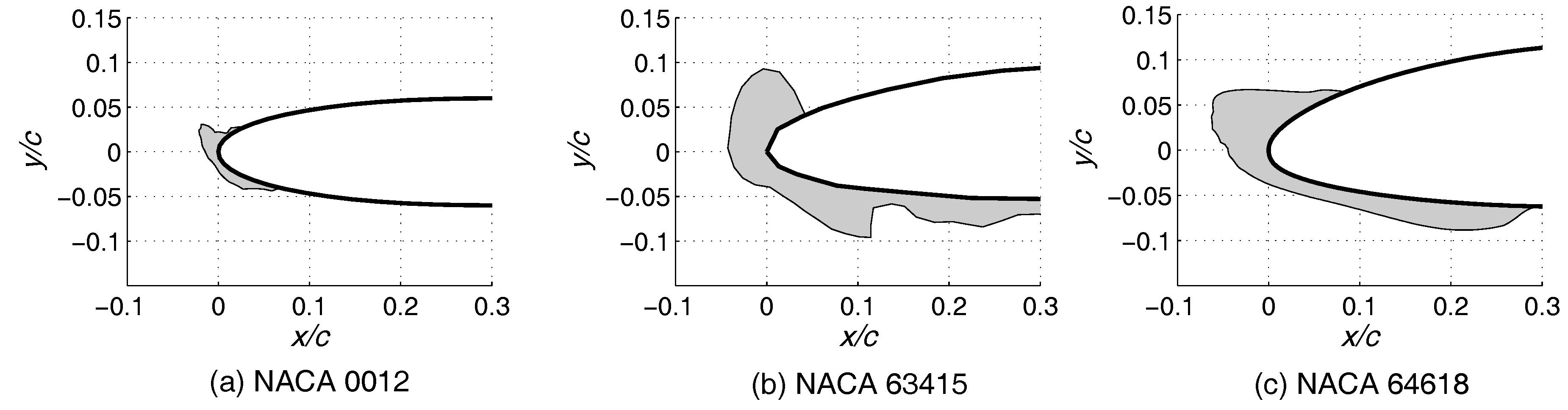
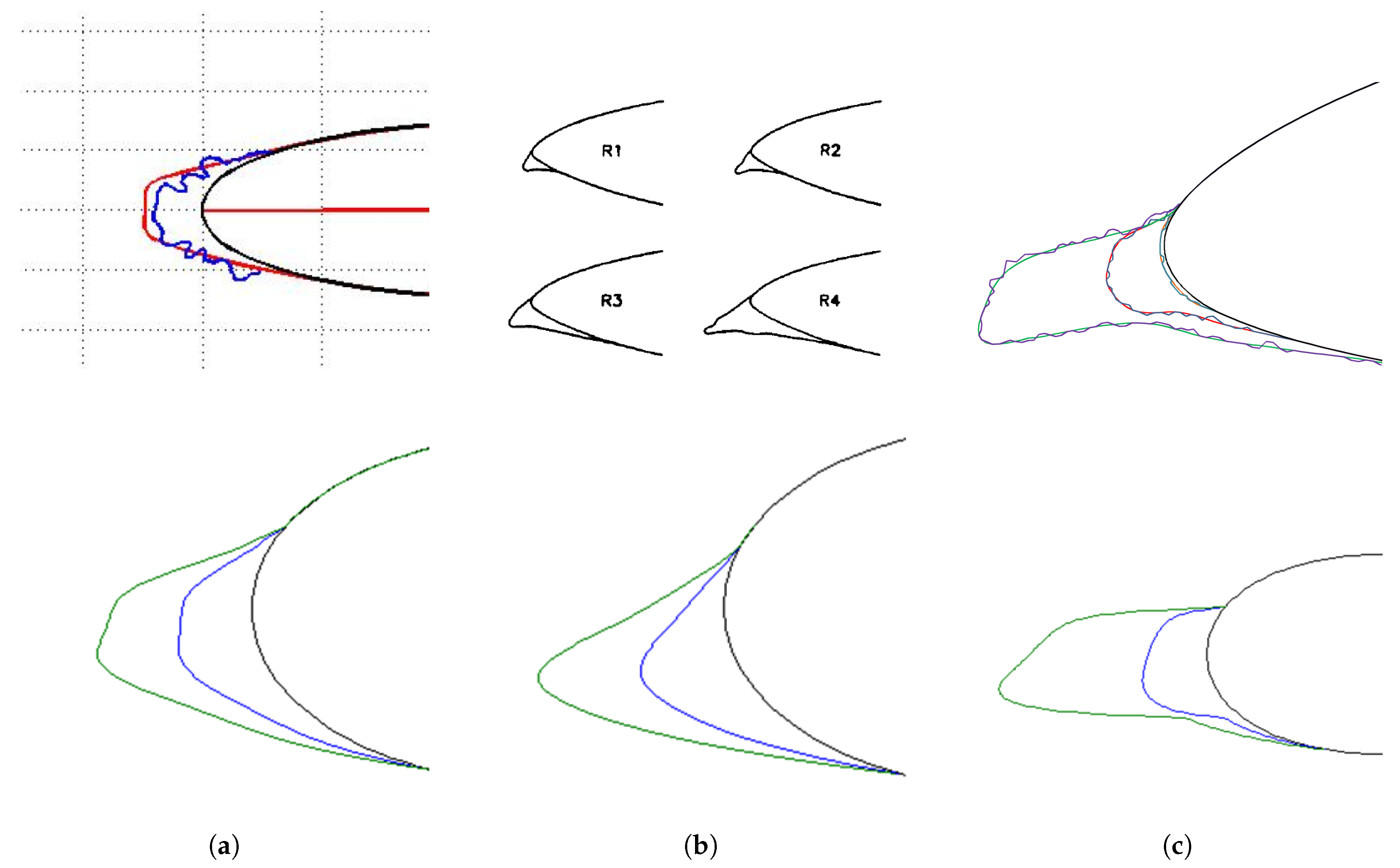
Wind turbines accumulate two types of icing: glaze and rime ice. Freezing rain or in-cloud icing creates smooth evenly distributed glaze ice (along chordwise). Super-cooled fog or cloud droplets form rime ice which is a most-common form of in-cloud icing. The rime ice accrete on the windward side of blade’s leading edge in the form of a wedge-shape. Ice accumulation on the blades depend on operating conditions of the turbine (ambient temperature, moisture content of the air, turbine speed, wind speed and the span of icing event) and geometric parameters (radial location, thickness, and chord length of aerofoils). The operating conditions of a turbine vary stochastically in space and time. Tools such as LEWICE [18], TURBICE [5], FENSAP-ICE [19] predict atmospheric icing of the blades using Multi-physics analysis involving heat transfer and CFD approach. These tools require wind speed, ambient temperature, liquid water content (LWC), median volume diameter (MVD) or droplet size and duration of the icing event as an input for prediction. These parameters change with wind turbine sites and they will be different for turbines within the site. This fact is also complemented by different ice fragments collected around a wind farm in [20]. Beaugendre et al. [19] predicted an ice shape as shown in the Figure 1a on a NACA 0012 aerofoil using ambient conditions (which are closer to the conditions that lead to glaze ice) given in Table 1 using FENSAP-ICE tool. Hochart et al. [7] used ambient conditions given in Table 1 (correspond to a severe icing event in Quebec during the winter in 2004–2005) in a wind tunnel and obtained ice shapes on a NACA 63415 aerofoil. The shape of accreted rime ice in their study is shown in the Figure 1b. The ice shape obtained in these studies can be very different if any of the parameters given in Table 1 is changed.
In this study, instead of predicting ice shapes using these parameters, a parametric model is developed to create a smoother ice shape as shown in the Figure 1c, approximately replicating the ice shapes shown in Figure 1a,b. Two points A and B are defined on an aerofoil section as shown in the Figure 2a and an initial curve with radial distances with origin at O (midpoint of the line joining the points A and B) is defined for various points on the clean aerofoil section between the points A and B. A new curve for creating an ice shape on the aerofoil as shown in the Figure 2b is defined using Equation (1) in terms of sinusoids.
where , defines the distance between origin O and points on the iced and clean aerofoils between A and B respectively, is the angle made by the line joining a point (between A and B) on the aerofoil section and origin O with respect to the line , f is a scaling factor used to distribute the required quantity of ice mass on the aerofoil section, represents the coefficient of the ith sinusoid.
The coefficients of the sinusoids are scaled according to an exponential curve defined by where k is chosen as a parameter. The order of sinusoids i and the value of k used in the function and scaling factor f are the three parameters to be identified for creating the required ice shape on an aerofoil section. A value of 0.5 is chosen for k to make the process of finding i and f further easier.
An ice shape is created on the NACA 64618 aerofoil (used on the NREL 5 MW wind turbine blade) by considering four sinusoids () in Equation (1), which is found by trial and error method to roughly replicate the ice accretion on the windward side of the aerofoil at leading edge as shown in Figure 1a,b. The coefficients of these four sinusoids are scaled according to an exponential function as shown in the Figure 3. The scaling factor f is determined by minimizing a cost function defined in MATLAB (8.3, MathWorks) using Equation (2) (product of the area of ice shape and its density is equated to ice mass) for a desired quantity of ice mass to be distributed on that section.
where , are the ice mass (per unit length) to be distributed on the aerofoil section and density of the ice respectively.
The ice shape in Figure 3 is obtained with the values of kg/m, kg/m3. This parametric model can be used to replicate ice shapes measured directly on blades during the icing events or ice pieces collected around the turbine (see [20] for different ice fragments collected around a wind farm) due to ice shedding. A few ice shapes obtained using some ice accretion simulations in the literature are replicated using the current parametric model in Appendix A.
The ice accumulation on wind turbines is influenced by many parameters (refer Table 1). It increases for longer icing events and it is not uniform across the blade length. Three different guidelines for the ice mass accumulation are defined in the literature: ISO 12494:2001 [21], GL [17] and VTT [13] formulas. Rissanen et al. [13] used these three formulas to calculate ice mass distribution on a 2.05 MW wind turbine blade. Based on the dimensions of turbine and span of icing events, these guidelines calculate maximum ice mass accumulation possible. The formula proposed in ISO 12494:2001 estimates ice mass based on the duration of icing event, chord length of the aerofoils and wind speed. This guideline estimates higher ice mass for longer icing events and blade root accumulates more ice mass as per this guideline due to its larger chord length. Wind turbine’s loads and vibrations are influenced by blade icing. GL [17] proposed a guideline to certify wind turbines for cold-climate operation. This guideline estimates maximum ice mass distribution possible on the blade that can be used to calculate turbine loads under different load cycles. Turbines accumulate ice mass lower than this limit, but it is used for certification of turbines under cold-climate operation. In reality, outer length of the blade i.e., near the tip accumulate more ice mass as this part of the blade sweeps more area in rotation and relative velocity of the wind is higher at these locations. This type of ice mass distribution is modeled by the GL guideline and it defines a linearly increasing i.e., mass distribution starting from zero at the blade root till a value of at half length of the blade. Thereafter it is constant towards the blade tip as shown in the Figure 4. The formula for calculating the value of is as follows [17]:
where is the ice mass density (700 kg/m3); , R is the rotor radius expressed in m, = 1 m; , are the maximum and minimum chord lengths of the blade expressed in m.
The value of for the NREL 5 MW wind turbine blade is calculated as 40.7 kg/m which estimates an ice mass of 1877 kg (it is equal to 10.58% of blade mass). Using this guideline, ice shapes are created on several sections of the current NREL 5 MW wind turbine blade as shown in the Figure 4 using the parametric model previously presented. This blade is described using 15 aerofoil sections with different shapes and chord lengths as shown in the Figure 4 whose details can be found in [22] and also given in the Table A1 in Appendix B. The aerodynamic behavior of these 15 aerofoil sections without and with ice are analyzed using the CFD simulations described in the next section.
3. Aerodynamic Characterization of Iced Aerofoils
The performance loss due to icing can be studied through different approaches, such as SCADA measurements, wind tunnel assessments, and numerical simulations. Experimental methods are the most realistic but are expensive. Wind tunnel tests have the advantage of a controlled environment, but problems are encountered in reproducing actual wind farm conditions and scaling certain dimensions and operating parameters. “Numerical methods offer the advantages of low cost and the ability to simulate realistic conditions, although efforts are still being made to develop these methods” [23]. The accuracy of simple numerical methods, such as panel codes, decreases for aerodynamic performance calculations of aerofoils, where thick trailing edges are considered. Also, they are not applicable for relative thicknesses greater than 30% to 36% [24]. Furthermore, these methods are not stable enough to work in the case of complicated ice profiles. CFD simulations with the Reynolds-Averaged Navier–Stokes (RANS) model is an alternative. However, CFD simulations accuracy depends on the quality of the grid system used for resolving the computational domain, as well as the appropriateness of the turbulence model in capturing the relevant physics [25]. Simulation of air flow around aerofoils using CFD has been studied by several researchers [26,27,28,29]. It is a challenge for the CFD-RANS model to simulate flow over thick aerofoils. The wind turbine blade region near the root is composed of thick aerofoil sections. The maximum relative thickness affects flow regime over an aerofoil and its aerodynamic characteristics. The location and size of the laminar separation bubbles are influenced by this parameter, as well as the transition. In the case of thick aerofoils, a fully developed turbulent boundary layer on the aerofoil surface was not found accurate enough to evaluate lift coefficient [24]. Due to the unavailability of experimental data in most of the real icing conditions, the accuracy of CFD predictions cannot always be validated. But there are some CFD studies [30,31,32,33,34] on iced aerofoils that have been validated with available experimental data. Their results show that a high-quality mesh is necessary, especially in the case of large horn ice shapes; as well as an appropriate turbulence model in addition to a transition model. In 2018 [12], total power loss was calculated for an iced NREL 5 MW rotor. They calculated rotor power using the BEM method in which 2-D aerofoil aerodynamic data were calculated using the CFD-RANS simulations. The validation was based on the clean aerofoils and did not include the icing results. Shu et al. [35] validated a 3-D CFD-RANS simulation on a 300-kW ice-contaminated wind turbine against the experiments. They found the glaze-iced rotor numerical results more overrated compared to the rime-iced one. They assumed a fully turbulent boundary layer skipping the laminar, turbulent transition. In summary, if there are no large separated regions, then CFD can accurately predict the loads, but it is also necessary for a CFD-RANS simulation to be reliable in the case of thicker aerofoils or/and sharp glaze ice profiles in which there are large separation regions or/and flow is not fully turbulent.
The mesh (spatial discretization) used in a CFD simulation should resolve the fluid domain around the aerofoil. It enables the governing equations with a turbulence model to resolve all the relevant physics with a minimum induced error. The task is challenging for the ice-contaminated aerofoils because of the complex geometry and flow. Furthermore, over a blade consisting different aerofoil geometries along the blade axis, ice profiles are thus different. An efficient mesh updating method for this purpose is thus necessary. A method was presented in [25] to generate a high-quality single- and multi-block structured grids for complicated 2-D ice profiles. The convergence was either extremely slow or did not converge because the coupled solver implemented computations in only one block at a time. In 2014 [36], a mesh morphing-based technique was described to effectively manage ice accretion simulations through the CFD. However, the stability of the method was not guaranteed as morphing typically introduces a degradation of the mesh quality. In 2016 [37], one CFD ice accretion model was designed, in which an ice accretion process was combined with the aerodynamic analysis. In this method, the mesh was updated by a node displacement vector at every time step.
With the above background, some improvements are necessary to improve CFD-RANS simulations in the case of separated flows, such as flow over thick aerofoils and flow at high angles of attack. Iced aerofoils are also profiles prone to separation, which makes CFD-RANS simulations challenging. The literature suggests modeling the boundary layer transition, using a proper turbulence model, improving the mesh quality etc. are necessary to make the CFD-RANS simulations as accurate as possible in such cases. The current study considers these measures to handle flow separation in the case of thick and iced aerofoil sections and are explained in the following subsections.
For the present study, a script-based method is used to modify the aerofoil/ice profile while preserving the mesh topology. Once the aerofoil profile is modified, only the node positions are rearranged and updated. Large number of CFD simulations are required considering different sections along the blade axis, range of angle of attack and ice profiles. The NREL 5 MW wind turbine blade is divided into 15 aerofoil sections (shown in Figure 4); ice accretion is different on these sections and require aerodynamic data on a range of angles of attack. Therefore, an automatic simulation is necessary along with an automatic mesh updating method. The whole process of the CFD simulations is controlled through a code developed in MATLAB. It consists of geometry update, mesh generation, solver setup, solver operation, and post processing of results. This is the novelty of the current work which launches a setup for the whole process of CFD-RANS simulations to analyze aerodynamic behavior of a wide range of aerofoil profiles.
3.1. Approach and Methods
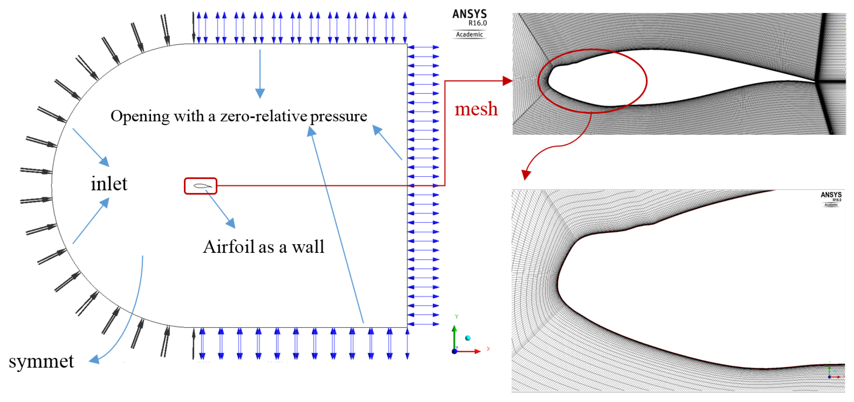
The NREL 5 MW wind turbine blade is constructed based on five “DU” aerofoils and one “NACA64” aerofoil. The maximum relative thickness of the cross-sections ranges from 18% to 40%. Design of the aerofoil profiles used in the blade are based on DU 99, DU 97, DU 91, DU 93 and NACA 64618 for which the experimental data are available in [38,39,40,41]. These aerofoils are finally named DU40_A17, DU35_A17, DU30_A17, DU21_A17, NACA64_A17 after some modifications such as the reduction in trailing edge thickness, aspect ratio, etc. [42]. Over 22% of the blade length, the maximum relative thickness on the cross-sections is greater than 30%. Such a geometry limits the application of aerodynamics modeling tools. The computational domain around the two-dimensional aerofoil contains a multi-block structured grid which consists of an unstructured arrangement of 10 hexahedral blocks. Each block contains a structured grid, created in the ICEM CFD (15.0, Ansys Inc., Canonsburg, PA, USA) software. The multi-block topology employed for this work starts from a C-topology around the aerofoil, see Figure 5. This arrangement helps to resolve the suction peak as well as the trailing edge vortex shedding. Such topology avoids low-quality hexahedral cells around the extremely sharp trailing edge geometry at the blade tip. The average y+ value on the blade is below 1 over the 0.5 million nodes of the mesh. Grid sensitivity study was implemented for the simulations of the basic (ice-free) profiles. The results were validated against the experimental data. For the iced profiles, the results stability was assessed with an emphasize on the worst cases, i.e., flow at high angle of attacks. The fluid problem is solved with the finite volume technique using the CFD code ANSYS CFX (15.0, Ansys Inc.) in which the set of equations is the Navier–Stokes equations in their conservation form [43]. The high-resolution advection scheme was selected for the spatial discretization. The temporal discretization of the equations in transient cases were solved using the second order backward Euler scheme. Considering the Reynolds-Averaged Naiver-Stokes equations, the turbulences were modeled with an eddy-viscosity model. The Shear Stress Transport (SST) model with an automatic wall function was activated to model the turbulent flow. The k- SST model is known to be an accurate turbulence model for boundary layer detachment prediction [44,45]. In a steady-state simulation, CFD solver applies a false time step as a mean of under-relaxing the equations, assuming that the equations iterate towards the final steady-state solution. To provide enough relaxation for the non-linearities in the equation, a small size of the physical time scale is applied, so that a converged steady-state solution is obtained. In this way the solution has evolved with ’time’ to provide transient information on a time-dependent phenomenon [43]. In this work, a sensitivity analysis was performed to ensure the independence of the results from the size of physical time scale. Running the transient simulations in a few random cases, similar load values were obtained. To reduce the computational time, steady-state simulations were implemented. “The adequate modeling of laminar/turbulent transition is important for the correct prediction of wall-bounded flows as the transition substantially influences the skin friction and therefore the energy losses” [46]. The separation point/line can change significantly between laminar and turbulent flows. Therefore, the transition modeling affects the simulation of the boundary layer separation. Some laminar/turbulent transition models are based on the intermittency coefficient. Others are defined by a three-equation model with an extra equation for the energy of non-turbulent fluctuations [46]. The transition model in this study is based on an experimental correlation concept. It is called the “Gamma-Theta Model” which is the recommended transition model for general-purpose applications [43]. The full model is based on two transport equations for the intermittency and the transition onset. The criterion for this transition onset is defined in terms of the momentum thickness Reynolds number.
The boundary conditions are set to be as followings which are also shown in Figure 5. The outlet of the domain is defined as an “opening” type. which allows the flow to cross the boundary in either direction. Domain inlet is described with a predefined axial velocity based on the required Reynolds number at each cross section. Aerofoil is a “no slip wall”, surrounding borders are “opening” and the span direction sides are set to be “symmetry” type.
3.2. Validation
Ruud van Rooij [42] provided 2-D measured coefficients for the DU-aerofoils for a Reynolds number of 7 million. To ensure the validity of the employed CFD simulation method, the calculated load coefficients are compared to the experimental data at the available range of angle of attack in Figure 6. The reported experimental data were digitized from the corresponding reference. Regarding the structural design of NREL rotor, radial sections near the tip are slender while they increase in thickness at lower radius to finally become circular at the blade root. As previously mentioned, more numerical considerations are necessary for thick clean aerofoils due to the more severe separation. On the other hand, aerofoil sections at the higher radius are the critical sections in the case of icing as they are prone to severe ice accretion compared to the root ones. Accordingly, two sample cases, one near the tip and one near the root are shown in the Figure 6. The validation study is implemented for all the profiles, not shown here. The CFD results are in good agreement with the measured ones for the lift, drag and moment coefficients.
3.3. Output
The simulation on the lower radius sections shows that the flow is not fully turbulent on the blade. Regarding Gamma-theta model, the transition points are shown in the Figure 7 (left). Neglecting the laminarity of the flow near the leading edge, imposes a higher wall shear magnitude on these regions (Figure 7-right). This higher wall shear stress leads to an earlier separation and a larger vortex near the trailing edge. Consequently, the load coefficients are affected. Being validated by the experimental data, the Gamma-theta model works as a reliable model to simulate the transition process in this study.
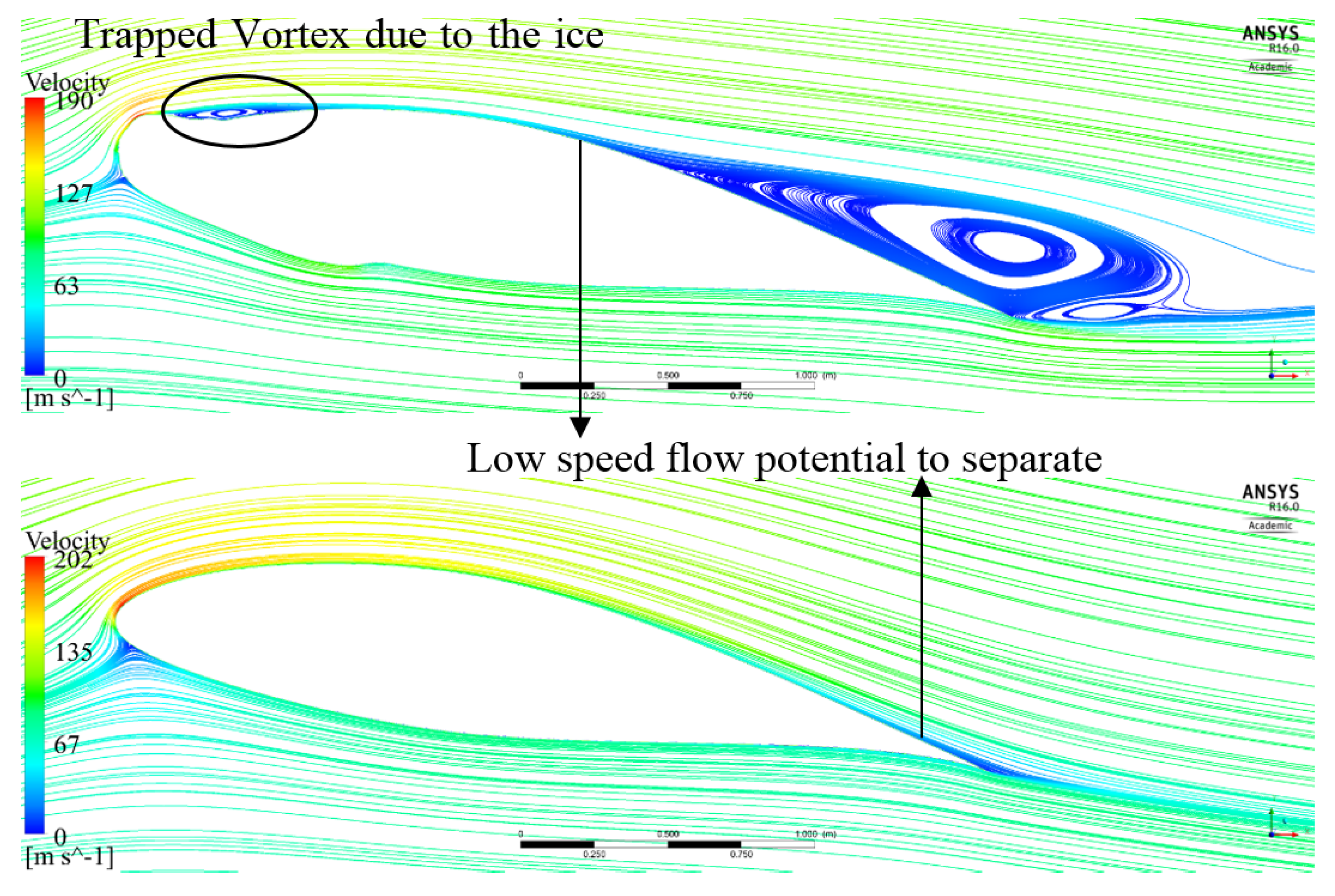
The flow visualization (Figure 8-top) demonstrates that icing effects are not limited to the leading-edge region, though the glaze ice accretes on the leading edge. First, a small vortex is trapped at the hinge of the upper horn. Downstream of the trapped vortex, the flow momentum is low, and is prone to separation. For the clean aerofoil (Figure 8-bottom), this condition occurs near the trailing edge, i.e., the flow momentum is sufficient to keep the flow attached up to the trailing edge.
The generated vortices affect the pressure distributions and consequently the aerodynamic forces on the aerofoil. Figure 9 shows the pressure distribution on the aerofoil from the leading edge to the trailing edge. The clean aerofoil is at a high angle of attack, as well as the glaze-iced one. Negative values of the pressure define the conditions below the ambient pressure, which is known as “suction”.
Upper (leeward) surface: The separation leads to a decrease in suction on this side of the aerofoil. While the flow passes the upper ice-horn from c to d in Figure 9, a noticeable reduction in the suction pressure arises. As described in the Figure 8, there are two vortices: a small one at the hinge of the horn, and a bigger one before the trailing edge. A reattached zone is found in the middle. The slope of pressure variations in the attached region () is similar for the clean and iced profiles, because the flow almost follows the curvature of the aerofoil in both clean and iced cases. In the second separated region (from e to the trailing edge) flow does not follow the designed aerofoil curvature and the pressure plots are so different, and they are crossing each other.
Lower (windward) surface: The different curvature of the ice from the leading edge to a, imposes a longer route for the flow compared to the clean case. Consequently, the flow accelerates leading to a lower pressure in this region. Since the flow is not separated, the pressure level recovers once the ice profile ends at b. This process decreases part of the potential lift by a local decrease in the pressure of the lower surface. Then from b to the trailing edge, the slope and the magnitude of pressure plots are similar for the clean and iced ones.
Altogether, the surface integration of the pressure distribution is less in the case of iced aerofoil. Lift, drag and moment variations are plotted in a range of angle of attack for a random section (Section 9) in Figure 10. The general effects of icing are decrease in lift forces and increase in drag forces. For the discussed ice profile, operating at a negative angle of attack can almost skip the effect of icing, while with increasing the positive angle of attack, a substantial part of the performance is lost. This is due to an earlier stall in the case of icing.
4. Results and Discussion
To support concept studies for offshore wind technology, Jonkman et al. [22] developed specifications for a multi-megawatt turbine and referred it as NREL offshore 5 MW baseline wind turbine. The onshore version of this turbine is analyzed in this study using the FAST v8.16 [47] tool to analyze its aeroelastic behavior. This tool consists of various sub-modules to model structural, aerodynamic; control and electrical-drive dynamics and all these modules are coupled to each other. The theory and implementation details of these modules in the FAST tool can be found in [47]. The NREL 5 MW wind turbine model with clean and iced blades is analyzed in this section considering 2-D static aerodynamic coefficients of their aerofoils calculated using the CFD simulations described in the last section. These aerodynamic coefficients computed at limited angles of attack (−10° to 10°) are extrapolated for angles between −180° and 180° using Viterna’s extrapolation method [48] used in the QBlade [49]. The blade’s sectional properties such as mass density, polar mass moment of inertia, and center of mass are recalculated by assuming the ice mass is concentrated at a point on the leading edge of the aerofoil sections. These modified properties are used in the generalized sectional mass matrix (see Equation 3.9 in [50]) definition of the finite element model of the iced blade in FAST tool.
4.1. Effect of Icing on the Turbine Loads and Power
Initially, steady-state characteristics of the NREL 5 MW wind turbine model with clean and iced blades are analyzed at wind velocities in the range 3–12 m/s. The mechanical power generated by the turbine at these wind speeds is compared in Figure 11 and other steady-state characteristics (generator power, rotor torque, rotor thrust) are compared in the Figure 12. Iced turbine simulations show that it produces 38% less power compared to the clean blades case (averaged over the speed range 3–12 m/s) considering ice mass distribution used in this study. The turbine’s speed and power output steadily increase from the cut-in wind speed of 3 m/s till its rated wind speed of 11.4 m/s in the case of clean blades. The angle of attack on aerofoil sections also steadily increases from cut-in to rated wind speed, and thereafter reduces due to the pitching of the blade where the turbine’s power is limited to its rated power. The ice accumulation on the aerofoil sections reduced lift forces and increased drag forces. As a result, the generator power, rotor torque, and thrust loads are decreased in the case of wind turbine with iced blades. Iced turbine produces rated power at a wind speed above its rated wind speed, so turbine blades will not be pitched till that wind speed. As a result, the angle of attack on iced aerofoil sections of the blade increased even above the rated wind speed and their values in this study are exceeding the range of angles (−10° to 10°) evaluated by CFD. Due to the fact that the simulations in this section are restricted till rated wind speed of the turbine. The generator torque controller of a variable-speed wind turbine operating between cut-in and rated wind speeds finds an optimum speed of the turbine that produces a maximum power. The NREL 5 MW wind turbine controller finds lower rotational speed of the turbine as an optimum operating point in the case of iced blades (refer Figure 12) in contrast to the clean blade’s case. These simulations considered uniform ice on all three blades, which is highly unlikely. Any deviation from this assumption increases vibrations and loads acting on the turbine stationary components.
In the current study, ice mass is distributed on the blade using the GL specification. According to this specification, the larger aerofoil sections near the blade root accumulate less ice, whereas smaller aerofoil sections near the blade tip accumulate more ice as they sweep through a larger area in rotation. Thus, the aerofoil sections in the outer length of the blade are more distorted due to ice when compared to those near the root. This type of ice mass distribution can be qualitatively described as light icing in Zone 1, moderate icing in Zone 2 and severe icing in Zone 3. The aerodynamic behavior of the aerofoil sections along the three different zones of the blade (refer Figure 4) are changed differently due to ice. The individual contribution from these three zones to the turbine power in the clean and iced blades cases are shown in the Figure 13. The lengths of these three zones are approximately equal to 1/3rd of the blade length. The rotor power is mainly produced from zones 2 and 3 in the case of clean blades. As per the GL ice mass specification, the blade sections in Zone 3 are more distorted due to the ice presence, so the power production from this part of the blade is mostly reduced. The power production from zones 1 and 2 are not significantly changed due to ice. The angle of attack on the aerofoil sections along the blade increases due to the reduction in rotor speed of the iced turbine. Also, the resultant relative velocity of the wind at the aerofoil section is decreased. The reduction in lift forces due to a lower relative velocity at sections in zones 1 and 2 is compensated by an increase of the lift forces due to a higher angle of attack. As a result, the power production from zones 1 and 2 is not significantly changed due to ice. However, the lift curves of the aerofoil sections in Zone 3 are significantly affected as shown in the Figure 14 due to the ice and produces lower lift forces (in comparison to the clean blade) even at an increased angle of attack.
4.2. Effect of Icing on the Modal Behavior
The aeroelastic property changes in the blade due to ice affect its modal behavior (natural frequencies and damping factors). The increase in blade mass due to ice accumulation reduces its natural frequencies and the distortions in aerofoil shapes of the iced blade reduces its damping factors as the aerodynamic loads contributing to damping in the structure are reduced. The influence of icing on the modal behavior of the NREL 5 MW wind turbine blade is analyzed in this subsection using eigenvalue analysis of the linearized representation of its aeroelastic model. The nonlinear model of the turbine is linearized using the FAST linearization option about the turbine’s operating point in the steady winds. More details on the linearization procedure in FAST can be found in [51]. As the turbine structure consists of both rotating (blades) and non-rotating (tower) sub-components, the blade’s vibration degrees of freedom (DOF) defined in the rotating frame of reference are transformed into multi-blade coordinates (MBC) so that the equations of motion can be expressed in the stationary frame of reference. MBC transforms the blade’s vibration modes to rotor assembly modes, known as collective, progressive and regressive modes which couples the rotor to the remaining turbine structure [52]. Eigenvalue analysis of the linearized equations of motion in MBC are carried out with clean and iced blades. The aeroelastic natural frequencies and damping factors of the turbine vibration modes are plotted in Figure 15.
The aeroelastic natural frequencies of the iced blade are reduced due to an increase in its mass. Also, the nature of variation (slope) in frequency values with respect to the wind speed has also changed as the turbine operates at lower rotational speed with ice (refer rotor speed plot shown in Figure 12) and mass distribution of the blade changed due to ice. Flapwise vibration modes of the blade are highly damped especially the first flapwise mode and edgewise vibration modes are relatively lightly damped. The damping factors of iced blade’s flapwise vibration modes are approximately dropped to 1/3rd of the corresponding values of the clean blade. The slopes of aerodynamic coefficient curves (lift, drag and pitching moment coefficient curves plotted with respect to angles of attack) at the turbine’s operating point dictate the damping in turbine’s structure [53]. These slopes are changed due to ice (refer to iced aerofoil’s lift curves shown in Figure 14), as a result damping in the system is reduced as shown in the Figure 15 (modal behavior plot). Therefore, the iced turbine blades vibrate with higher amplitudes compared to the clean turbine, no ice, if similarly, excited. Severe icing on the blades reduces the rotational speed of the turbine and aerodynamic loads acting on the blade. The loads and vibrations of the remaining turbine structure (i.e., tower, hub, etc.) will also see a similar effect due to ice if it is symmetrical on all three blades (this case is highly unlikely in reality). Otherwise, the imbalance in structural mass or/and aerodynamic loads of the rotor due to icing can cause severe vibrations in the turbine’s structure. One severe risk associated with iced turbine blades is the ice throw which limits its operation, some countries have strict regulations to shut down the turbine once icing is detected.
Ice accumulates on the blades non-uniformly, and also its distribution changes under different stages of icing. Five different cases of the turbine model with clean and iced blades (full and partially iced) are analyzed for investigating the effect of icing on the damping factors of the blades’ vibration modes. These cases consider ice mass and aerofoil shapes as shown in the Figure 4. Among these, three cases consider partial icing where ice is present in zones 1–3 exclusively (remaining part of the blade is not iced). The turbine’s operating conditions (rotational speed) in these five cases will be different and thus the angles of attack at the aerofoil sections along the blade will also be different. These values at wind speeds of 6 and 10 m/s are shown in the Figure 16. In addition to that, the aerodynamic coefficient curves of aerofoil section changes due to ice so the slopes of these curves at the turbine’s operating conditions would be different. As a result, the modal damping factors of the blade’s vibration modes change as shown in the Figure 17 with the nature of icing (full and partially iced scenarios). The turbine power output in the case of fully iced blades (refer Figure 13) is dropped due to a lower power production from Zone 3. The power production from the other two zones is not significantly reduced due to the presence of ice. The power production with partial icing in only Zone 3 reduces in a similar way as the fully iced blade case, it emphasizes that aerodynamic forces on the blades are similar in those two cases. Due to the fact that similar reduction in the damping factors is observed in both cases. Moderate ice in only Zone 2 does not reduce the turbine power output, but the damping factors are marginally reduced as slopes of the aerodynamic curves at the increased angle of attack are different (small change only) than those correspond to a clean blade. The aerodynamic behavior of the blade with light icing in only Zone 1 is not changed significantly due to ice, as a result, the damping factors in this case coincide with the clean blade’s case.
Wind turbines operate under turbulent wind conditions which excite lowest natural frequencies of the blade. These frequencies can be extracted from the vibration measurements of the blade. These frequencies reduce with ice accumulation. Few ice-detection systems are available in the market [54] which monitor these frequencies to indicate the state of icing such as ice-free, non-critical, and critical ice. In this study, the blade vibrations are simulated over a duration of 500 s using the FAST tool with a turbulent wind profile over the rotor area with a mean wind speed of 8 m/s and a turbulent intensity of 10% considering clean and iced blades. The blade vibration accelerations (defined in the rotating frame of reference) at 6 different locations along the blade obtained from the simulations are used in the frequency-domain decomposition (FDD) technique to extract modal frequencies of the blade. The authors used an open-source MATLAB code [55] for modal parameter identification using the FDD. Further theoretical details on the FDD technique can be found in [56]. First singular value of the power spectral density (PSD) matrices at various frequencies calculated with simulated vibrations of the clean and iced blades are shown in the Figure 18, where natural frequencies of the blade are identified at the peaks in those plots.
The first flapwise vibration mode of the clean blade is highly damped, so it is not clearly identified from the 1st singular value plot of the PSD matrix calculated using flapwise vibrations of the blade in Figure 18 (top-left), whereas other higher modes can be easily identified as they are lightly damped. As icing reduced the damping factor of the first flapwise mode (refer Figure 15), a peak appears at the corresponding frequency in the 1st singular value plot of the PSD matrix in Figure 18 (bottom-left). The edgewise vibration modes are lightly damped, so they can be identified as shown in the Figure 18 (right) by applying the FDD method on the edgewise vibrations of the blade. Two peaks appear on either side of the first edgewise natural frequency of the blade at frequencies plus and minus of the rotational frequency in Figure 18 (right). The equations of motion governing the vibration behavior of the wind turbine structure are periodic due to the gravitational loads and wind shear. Time-periodic systems will have periodic mode shapes at frequencies which are the sum of the principal modal frequency plus or minus an integer multiple of the system frequency (here it is the rotational frequency of the turbine) leading to multiple resonances for a single vibration mode [57]. Out of these infinite harmonics, only a few of them will contribute to the vibration response [58]. The blade natural frequencies in Figure 18 are reduced differently for the ice mass distribution considered along the blade, this behavior changes for an ice mass distribution different from this. Gantasala et al. [59] proposed a technique to characterize the ice mass accumulated on the blades based on such changes in the natural frequencies with ice accumulation.
4.3. Asymmetrical Icing of the Blades
The results presented in the previous subsections are obtained considering uniform icing on all three blades which is highly unlikely. The asymmetrical icing on the blades can induce structural or/and aerodynamic imbalances in the rotor assembly. That means one blade may accumulate more ice mass or/and aerofoil shapes of one blade are more distorted due to the presence of ice. The dynamics of the wind turbine structure in such cases will be different when compared to the cases of clean and uniformly iced blades. To investigate the individual influence of structural and aerodynamic imbalances on the dynamic response of the turbine, ice induced changes in the structural and aerodynamic properties at specific locations of one blade are not considered in the simulation cases. Ice induced structural property changes in the Zone 2 region of one blade are not considered (that means it accumulates 35% less ice than the other two blades) in a simulation case to introduce structural imbalance in the rotor. Another case, where ice induced aerodynamic changes in the Zone 3 region of one blade are not considered in the model to simulate the influence of aerodynamic imbalance in the rotor on its dynamic behavior.
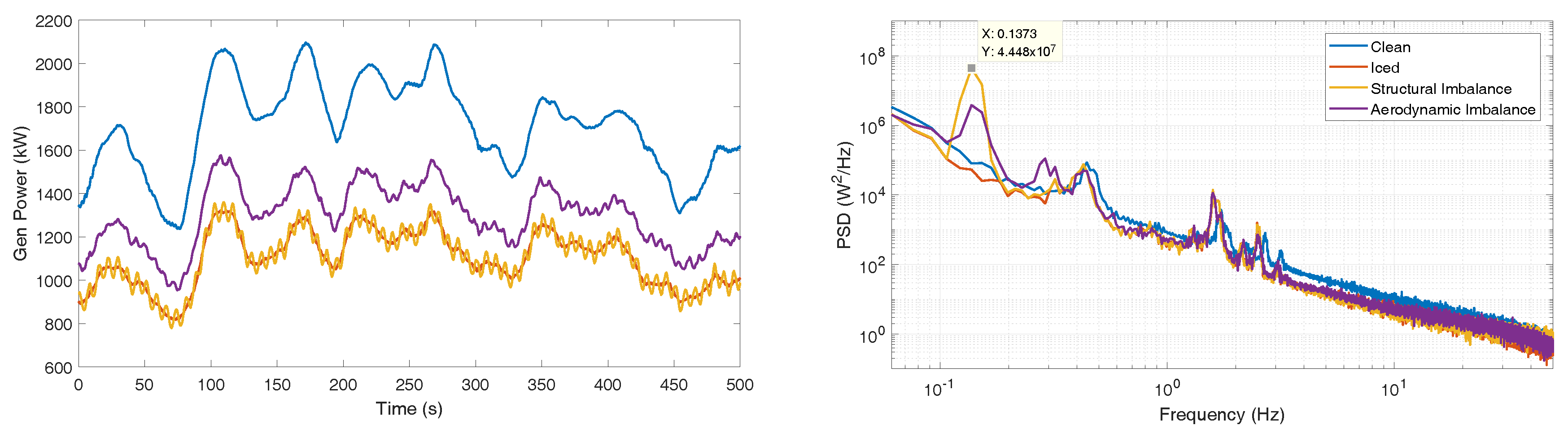
In addition to the turbulent wind response simulations carried out in the previous subsection with clean and uniformly iced blades, two simulations with iced blades considering structural and aerodynamic imbalances as described before are carried out. The generator power output over the simulated time in all these four cases and their power spectral densities (PSD) are shown in Figure 19. The clean turbine produces maximum power out of the four cases compared in this figure and the order of decreasing power output is followed by aerodynamic imbalance, structural imbalance, and uniformly iced cases. Icing of the blades reduces loads and vibrations if it is uniform on all three blades. However, structural and aerodynamic imbalances in the rotor assembly additionally induced low frequency oscillations (corresponding to the rotational speed of the turbine) in the power output (refer Figure 19-right). Similar behavior is observed in other dynamic parameters of the turbine (like rotational speed, thrust, torque etc.) with these imbalances.
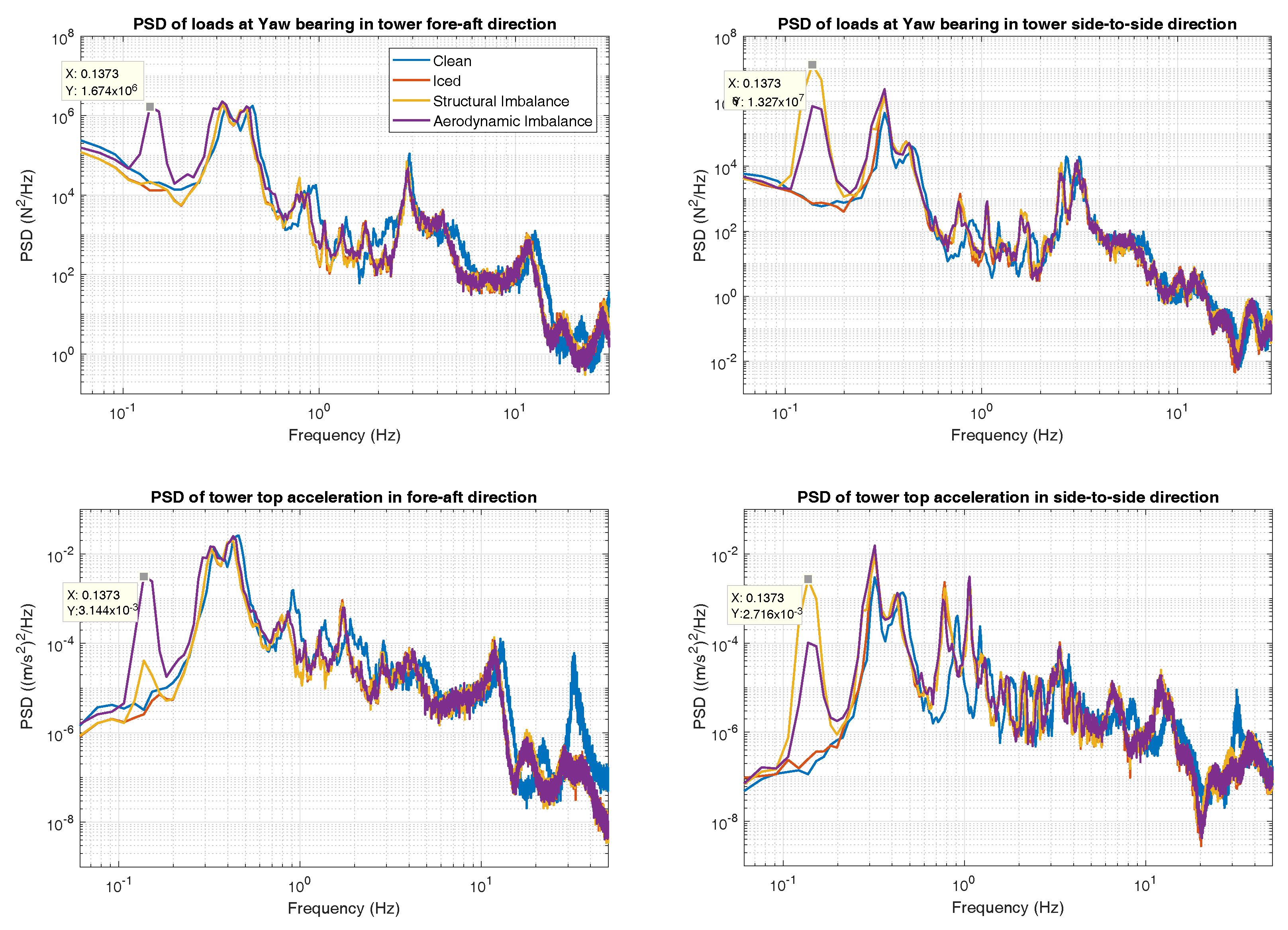
Structural and aerodynamic imbalances are not severely affecting the dynamic behavior of the blades. However, other structural components, tower, hub and nacelle assembly will experience additional loads (when compared to uniform ice on all blades) and vibrations due to these imbalances. The PSD of the loads acting on Yaw bearing and tower top vibration accelerations in the tower fore-aft and side-to-side directions are shown in the Figure 20. The structural imbalance induces oscillations with a frequency equal to the rotational speed of the turbine in the loads and vibrations of the tower in side-to-side direction. The aerodynamic imbalance induces oscillations in the loads and vibrations of the tower in the fore-aft direction. Due to the non-uniform ice accumulation on the wind turbine blades, additional loads, and vibrations are generated on the rotor assembly and tower structure. The turbine will be eventually shut down if these vibrations exceed a predefined threshold. These vibrations can also be monitored along with the power output of the turbine to detect icing of the blades more efficiently [60].
5. Summary and Conclusions
In this paper, a parametric model is fitted to an ice shape and scaled to add ice mass on the NREL 5 MW wind turbine as defined by the GL limit. The aerodynamic behavior of 15 clean and iced aerofoil sections is predicted using an automated CFD analysis at a few angles of attack between −10° and 10°. The laminar to turbulent transition on the aerofoil, critical near the hub, was modeled in all the simulations. The mesh near the tip is challenging to produce because of the ice shape. Ice profile changes the pressure distribution on the aerofoil and leads to a loss in the lift force and an extra drag. The reason is a large separation region over the blade and trapped vortices at the leading-edge ice. The GL limit considers more ice mass in the outer half of the blade which consists aerofoil sections with smaller chord length. Therefore, these aerofoil sections are more distorted due to ice. The last third of the blade in the current case has a larger drop in the power output which otherwise produces about 50% of the turbine’s power with clean blades. Icing reduces rotational speed and loads in the turbine. The power output from the inner two third of the blade length (starting from the root) in the current case did not reduce due to ice as the angle of attack in this part increased due to the low rotational speed. The reduction in lift force due to a lower resultant wind speed is compensated by an increase in the lift force by operating at a higher angle of attack.
Icing causes structural and aerodynamic property changes in the blade. The increase in blade mass due to the ice accumulation reduces natural frequencies of the blade and aerodynamic penalties due to the aerofoil shape distortion reduces aeroelastic damping in the blades. The influence of icing in three different locations of the blade is investigated on the aeroelastic damping factors of the blade’s vibration modes. Moderate icing in the middle third of the blade reduced these damping factors slightly, whereas severe icing in the outer third of the blade reduced damping factors of flapwise vibration modes by about 70%. Wind turbines usually operate under turbulent wind conditions whose wide frequency spectrum may excite lowest natural frequencies of the blade. The vibration accelerations of the blade simulated with a turbulent wind profile over the rotor area considering clean and iced blades in the current study are used in an FDD technique to extract modal frequencies of the blade. Vibration modal frequencies of the iced blade are reduced. These frequencies reduce differently depending on the nature of the ice mass (quantity and location) along the blade length. Therefore, these vibrations can be monitored to detect the presence of ice on individual blades in contrast to other methods that use power curve, rotational speed, pitch angle deviations from the reference values for ice detection on whole rotor.
Ice accumulation on the turbine blades is not uniform which can cause two types of imbalances in the turbine operation: structural and aerodynamic. These two imbalances are simulated in the current study by ignoring corresponding ice induced changes in a specific location of one blade. Icing of the blades reduces loads and vibrations if it is uniform on all three blades. The structural imbalance created by an asymmetrical ice mass on three blades causes additional loads and vibrations of the tower (when compared to uniformly iced case) in side-to-side direction, whereas the asymmetrical aerodynamic penalties in the rotor due to ice causes additional loads and vibration of the tower in the fore-aft direction. The tower or nacelle vibrations can be monitored along with a power curve-based analysis for an efficient and reliable ice detection.
The proposed methodology can be leveraged to analyze the influence of any ice shape, and ice mass distribution on the dynamic behavior of any wind turbine model due to the automated nature of ice shape scaling and CFD analysis of the iced aerofoil sections. The above conclusions are based on the simulations performed on the turbine model between cut-in to rated wind speed range.
Author Contributions
Conceptualization, S.G.; Investigation, S.G. and N.T.; Methodology, S.G. and N.T.; Software, S.G. and N.T.; Supervision, M.C. and J.-O.A.; Writing—original draft, S.G. and N.T.; Writing—review & editing, M.C. and J.-O.A.
Funding
This research was partially funded by Swedish Energy Agency.
Acknowledgments
This research work is carried out as a part of the project on “Wind power in cold climates” funded by the Swedish Energy Agency, which supports research and development investments in wind power.
Conflicts of Interest
The authors declare no conflict of interest.
Appendix A. Parametric Modeling of the Leading-Edge Ice Shapes Predicted in the Literature
Ice shapes from the simulations carried out in the literature are approximately replicated below using the parametric model described in Section 2 of the current work. The original ice shapes are shown in the top part of the Figure A1 and ice shapes obtained from the parametric model are shown in the bottom part of the Figure A1. Replicated ice shapes will not exactly match due to the differences in the aerofoil shapes used in the literature (top part of the figure) and the ones used in the parametric model (bottom part of the figure).

Appendix B. NREL 5 MW Model Wind Turbine Blade Data

Table A1.
Aerofoil details of the blade.
| Section Name | Radius (m) | Twist Angle (°) | Chord (m) | Aerofoil Name |
|---|---|---|---|---|
| Section 1 | 11.75 | 13.308 | 4.557 | DU40_A17 |
| Section 2 | 15.85 | 11.480 | 4.652 | DU35_A17 |
| Section 3 | 19.95 | 10.162 | 4.458 | DU35_A17 |
| Section 4 | 24.05 | 9.011 | 4.249 | DU30_A17 |
| Section 5 | 28.15 | 7.795 | 4.007 | DU25_A17 |
| Section 6 | 32.25 | 6.544 | 3.748 | DU25_A17 |
| Section 7 | 36.35 | 5.361 | 3.502 | DU21_A17 |
| Section 8 | 40.45 | 4.188 | 3.256 | DU21_A17 |
| Section 9 | 44.55 | 3.125 | 3.010 | NACA64_A17 |
| Section 10 | 48.65 | 2.319 | 2.764 | NACA64_A17 |
| Section 11 | 52.75 | 1.526 | 2.518 | NACA64_A17 |
| Section 12 | 56.17 | 0.863 | 2.313 | NACA64_A17 |
| Section 13 | 58.90 | 0.370 | 2.086 | NACA64_A17 |
| Section 14 | 61.63 | 0.106 | 1.419 | NACA64_A17 |
| Section 15 | 63.00 | 0.106 | 1.419 | NACA64_A17 |
References
- Lehtomäki, V. Emerging from the Cold. 2016. Available online: http://www.windpowermonthly.com/article/1403504/emerging-cold (accessed on 28 November 2017).
- Wallenius, T.; Lehtomäki, V. Overview of cold climate wind energy: Challenges, solutions, and future needs. Wiley Interdiscip. Rev. Energy Environ. 2016, 5, 128–135. [Google Scholar] [CrossRef]
- Fortin, G.; Perron, J.; Ilinca, A. A study of icing events at Murdochville: Conclusions for the wind power industry. In Proceedings of the International Symposium “Wind Energy in Remote Regions”, Magdalen’s Island, QC, Canada, October 2005. [Google Scholar]
- Homola, M.C.; Nicklasson, P.J.; Sundsbø, P.A. Ice sensors for wind turbines. Cold Reg. Sci. Technol. 2006, 46, 125–131. [Google Scholar] [CrossRef]
- Turkia, V.; Huttunen, S.; Wallenius, T. Method for Estimating Wind Turbine Production Losses Due to Icing; VTT: Espoo, Finland, 2013. [Google Scholar]
- Rindeskär, E. Modelling of Icing for Wind Farms in Cold Climate: A Comparison between Measured and Modelled Data for Reproducing and Predicting Ice Accretion. Master’s Thesis, Institutionen för Geovetenskaper, Uppsala Universitet, Uppsala, Sweden, 2010. [Google Scholar]
- Hochart, C.; Fortin, G.; Perron, J.; Ilinca, A. Wind turbine performance under icing conditions. Wind Energy 2008, 11, 319–333. [Google Scholar] [CrossRef]
- Yirtici, O.; Tuncer, I.; Ozgen, S. Ice Accretion Prediction on Wind Turbines and Consequent Power Losses. J. Phys. Conf. Ser. 2016, 753. [Google Scholar] [CrossRef]
- Homola, M.C.; Virk, M.S.; Nicklasson, P.J.; Sundsbø, P.A. Performance losses due to ice accretion for a 5 MW wind turbine. Wind Energy 2012, 15, 379–389. [Google Scholar] [CrossRef]
- Hu, L.; Zhu, X.; Hu, C.; Chen, J.; Du, Z. Wind turbines ice distribution and load response under icing conditions. Renew. Energy 2017, 113, 608–619. [Google Scholar] [CrossRef]
- Etemaddar, M.; Hansen, M.O.L.; Moan, T. Wind turbine aerodynamic response under atmospheric icing conditions. Wind Energy 2014, 17, 241–265. [Google Scholar] [CrossRef]
- Zanon, A.; De Gennaro, M.; Kühnelt, H. Wind energy harnessing of the NREL 5 MW reference wind turbine in icing conditions under different operational strategies. Renew. Energy 2018, 115, 760–772. [Google Scholar] [CrossRef]
- Rissanen, S.; Lehtomäki, V.; Wennerkoski, J.; Wadham-Gagnon, M.; Sandel, K. Modelling load and vibrations due to iced turbine operation. Wind Eng. 2016, 40, 293–303. [Google Scholar] [CrossRef]
- Han, W.; Kim, J.; Kim, B. Study on correlation between wind turbine performance and ice accretion along a blade tip airfoil using CFD. J. Renew. Sustain. Energy 2018, 10, 023306. [Google Scholar] [CrossRef]
- Shu, L.; Li, H.; Hu, Q.; Jiang, X.; Qiu, G.; McClure, G.; Yang, H. Study of ice accretion feature and power characteristics of wind turbines at natural icing environment. Cold Reg. Sci. Technol. 2018, 147, 45–54. [Google Scholar] [CrossRef]
- Lamraoui, F.; Fortin, G.; Benoit, R.; Perron, J.; Masson, C. Atmospheric icing impact on wind turbine production. Cold Reg. Sci. Technol. 2014, 100, 36–49. [Google Scholar] [CrossRef]
- Guideline, G.W.; Lloyd, G. Guideline for the Certification of Wind Turbines; Germanischer Lloyd Wind Energie GmbH: Hamburg, Germany, 2010. [Google Scholar]
- Wright, W.B. User Manual for the NASA Glenn Ice Accretion Code LEWICE Version 2.2; NASA: Washington, DC, USA, 2002.
- Beaugendre, H.; Morency, F.; Habashi, W. Development of a second generation in-flight icing simulation code. J. Fluids Eng. 2006, 128, 378–387. [Google Scholar] [CrossRef]
- Wadham-Gagnon, M.; Bolduc, D.; Boucher, B.; Camion, A.; Petersen, J.; Friedrich, H. Ice Profile Classification Based on ISO 12494. TechnoCentre éolien (Wind Energy TechnoCentre); WinterWind: Östersund, Sweden, 2013. [Google Scholar]
- ISO. Atmospheric Icing of Structures; International Standard; ISO: Geneva, Switzerland, 2001; Volume 12494. [Google Scholar]
- Jonkman, J.; Butterfield, S.; Musial, W.; Scott, G. Definition of a 5 MW Reference Wind Turbine for Offshore System Development; Technical Report; National Renewable Energy Laboratory (NREL): Golden, CO, USA, 2009.
- Tabatabaei, N. Impact of Icing on Wind Turbines Aerodynamic. Ph.D. Thesis, Luleå tekniska Universitet, Luleå, Sweden, 2018. [Google Scholar]
- Schubel, P.J.; Crossley, R.J. Wind turbine blade design. Energies 2012, 5, 3425–3449. [Google Scholar] [CrossRef]
- Chi, X.; Zhu, B.; Shih, T. Computing Aerodynamic Performance of a 2D Iced Airfoil: Blocking Topology and Grid Generation. In Proceedings of the 40th AIAA Aerospace Sciences Meeting & Exhibit, Reno, NV, USA, 14–17 January 2002. [Google Scholar]
- Kieffer, W.; Moujaes, S.; Armbya, N. CFD study of section characteristics of Formula Mazda race car wings. Math. Comput. Model. 2006, 43, 1275–1287. [Google Scholar] [CrossRef]
- Bai, Y.; Sun, D.; Lin, J.; Kennedy, D.; Williams, F. Numerical aerodynamic simulations of a NACA airfoil using CFD with block-iterative coupling and turbulence modelling. Int. J. Comput. Fluid Dyn. 2012, 26, 119–132. [Google Scholar] [CrossRef]
- Eleni, D.C.; Athanasios, T.I.; Dionissios, M.P. Evaluation of the turbulence models for the simulation of the flow over a National Advisory Committee for Aeronautics (NACA) 0012 airfoil. J. Mech. Eng. Res. 2012, 4, 100–111. [Google Scholar]
- Panigrahi, D.C.; Mishra, D.P. CFD Simulations for the Selection of an Appropriate Blade Profile for Improving Energy Efficiency in Axial Flow Mine Ventilation Fans. J. Sustain. Min. 2014, 13, 15–21. [Google Scholar] [CrossRef]
- Ma, D.; Zhao, Y.; Qiao, Y.; Li, G. Effects of relative thickness on aerodynamic characteristics of airfoil at a low Reynolds number. Chin. J. Aeronaut. 2015, 28, 1003–1015. [Google Scholar] [CrossRef] [Green Version]
- Villalpando, F.; Reggio, M.; Ilinca, A. Numerical Study of Flow Around Iced Wind Turbine Airfoil. Eng. Appl. Comput. Fluid Mech. 2012, 6, 39–46. [Google Scholar] [CrossRef]
- Chi, X.; Zhu, B.; Shih, T.I.P.; Addy, H.E.; Choo, Y.K. CFD analysis of the aerodynamics of a business-jet airfoil with leading-edge ice accretion. AIAA Pap. 2004, 560, 2004. [Google Scholar]
- Mortensen, K. CFD Simulations of an Airfoil With Leading Edge Ice Accretion. Ph.D. Thesis, Technical University of Denmark, Copenhagen, Denmark, 2008. [Google Scholar]
- Hudecz, A.; Koss, H.; Hansen, M. Ice accretion on wind turbine blades. In Proceedings of the IWAIS, St. John’s, NL, Canada, 8–11 September 2013; pp. 8–11. [Google Scholar]
- Shu, L.; Li, H.; Hu, Q.; Jiang, X.; Qiu, G.; He, G.; Liu, Y. 3D numerical simulation of aerodynamic performance of iced contaminated wind turbine rotors. Cold Reg. Sci. Technol. 2018, 148, 50–62. [Google Scholar] [CrossRef]
- Costa, E.; Biancolini, M.; Groth, C.; Travostino, G.; D’Agostini, G. Reliable Mesh Morphing Approach to Handle Icing Simulations on Complex Models. In Proceedings of the 4th EASN Association International Workshop on Flight Physics and Aircraft Design, Aachen, Germany, 27–29 October 2014. [Google Scholar]
- Pedersen, M.C.; Sørensen, H. Towards a CFD Model for Prediction of Wind Turbine Power Losses due to Icing in Cold Climate. In Proceedings of the 16th International Symposium on Transport Phenomena and Dynamics of Rotating Machinery, Honolulu, HI, USA, 10–15 April 2016. [Google Scholar]
- Abbott, I.H.; Von Doenhoff, A.E.; Stivers, L., Jr. Summary of Airfoil Data; Technical Report No. 824; National Advisory Committee for Aeronautics: Washington, DC, USA, 1945.
- Timmer, W.A.; Van Rooij, R.P.J.O.M. Summary of the Delft University wind turbine dedicated airfoils. Trans. Am. Soc. Mech. Eng. J. Sol. Energy Eng. 2003, 125, 488–496. [Google Scholar] [CrossRef]
- Van Rooij, R.P.J.O.M.; Timmer, W.A. Roughness sensitivity considerations for thick rotor blade airfoils. Trans. Am. Soc. Mech. Eng. J. Sol. Energy Eng. 2003, 125, 468–478. [Google Scholar] [CrossRef]
- Llorente, E.; Gorostidi, A.; Jacobs, M.; Timmer, W.A.; Munduate, X.; Pires, O. Wind tunnel tests of wind turbine airfoils at high reynolds numbers. J. Phys. Conf. Ser. 2014, 524. [Google Scholar] [CrossRef]
- Kooijman, H.J.T.; Lindenburg, C.; Winkelaar, D.; van der Hooft, E.L. Aero-elastic Modelling of the DOWEC 6 MW Pre-Design in PHATAS; Technical Report ECN-CX–01-135, EET Programme of the Dutch Ministry of Economic Affairs; Wind Energy; ECN: Petten, The Netherlands, 2003. [Google Scholar]
- Ansys, C. ANSYS CFX Solver Modeling Guide, Release 15.0; ANSYS Inc.: Canonsburg, PA, USA, 2013. [Google Scholar]
- Ducoin, A.; Astolfi, J.A.; Deniset, F.; Sigrist, J.F. Computational and experimental investigation of flow over a transient pitching hydrofoil. Eur. J. Mech. B/Fluids 2009, 28, 728–743. [Google Scholar] [CrossRef] [Green Version]
- Menter, F.R. Improved Two-Equation K-omega Turbulence Models for Aerodynamic Flows; NASA: Washington, DC, USA, 1992.
- Fürst, J.; Straka, P.; Příhoda, J.; Šimurda, D. Comparison of several models of the laminar/turbulent transition. EPJ Web Conf. 2013, 45, 01032. [Google Scholar] [CrossRef]
- Jonkman, J.; Jonkman, B. NWTC Information Portal (FAST v8). Available online: https://nwtc.nrel.gov/FAST8 (accessed on 28 November 2017).
- Viterna, L.A.; Corrigan, R.D. Fixed pitch rotor performance of large HAWTs, DOE. In NASA Workshop on Large HAWTs; NASA: Cleveland, OH, USA, 1980. [Google Scholar]
- QBlade v0.96.3. Available online: https://sourceforge.net/projects/qblade/?source=directory (accessed on 3 May 2017).
- Wang, Q.; Jonkman, J.; Sprague, M.; Jonkman, B. BeamDyn Users Guide and Theory Manual; National Renewable Energy Laboratory: Lakewood, CO, USA, 2016.
- Jonkman, J.M.; Buhl, M.L., Jr. FAST User’s Guide-Updated August 2005; Technical Report; National Renewable Energy Laboratory (NREL): Golden, CO, USA, 2005.
- Bir, G.S. User’s Guide to MBC3: Multi-Blade Coordinate Transformation Code for 3-Bladed Wind Turbine; National Renewable Energy Laboratory: Lakewood, CO, USA, 2010.
- Gantasala, S.; Luneno, J.C.; Aidanpää, J.O. Influence of icing on the modal behavior of wind turbine blades. Energies 2016, 9, 862. [Google Scholar] [CrossRef]
- Cattin, R.; Heikkilä, D. Evaluation of Ice Detection Systems for Wind Turbines; Meteotest: Bern, Switzerland, 2016. [Google Scholar]
- Cheynet, E. Automated Frequency Domain Decomposition (AFDD). Downloaded from MATLAB Central File Exchange. Available online: https://se.mathworks.com/matlabcentral/fileexchange/57153-automatedfrequency-domain-decomposition--afdd- (accessed on 3 May 2017).
- Brincker, R.; Zhang, L.; Andersen, P. Modal identification of output-only systems using frequency domain decomposition. Smart Mater. Struct. 2001, 10, 441. [Google Scholar] [CrossRef]
- Skjoldan, P.F.; Hansen, M.H. On the similarity of the Coleman and Lyapunov-Floquet transformations for modal analysis of bladed rotor structures. J. Sound Vib. 2009, 327, 424–439. [Google Scholar] [CrossRef]
- Bottasso, C.; Cacciola, S. Model-independent periodic stability analysis of wind turbines. Wind Energy 2015, 18, 865–887. [Google Scholar] [CrossRef]
- Gantasala, S.; Luneno, J.C.; Aidanpää, J.O. Identification of ice mass accumulated on wind turbine blades using its natural frequencies. Wind Eng. 2018, 42, 66–84. [Google Scholar] [CrossRef]
- Skrimpas, G.A.; Kleani, K.; Mijatovic, N.; Sweeney, C.W.; Jensen, B.B.; Holboell, J. Detection of icing on wind turbine blades by means of vibration and power curve analysis. Wind Energy 2016, 19, 1819–1832. [Google Scholar] [CrossRef]
- Brouwers, E.W. The Experimental Investigation of a Rotor Icing Model with Shedding. Master’s Thesis, The Graduate School College of Engineering, The Pennsylvania State University, State College, PA, USA, 2010. [Google Scholar]
- Jasinski, W.J.; Noe, S.C.; Selig, M.S.; Bragg, M.B.; Jasinski, W.J.; Noe, S.C.; Selig, M.S.; Bragg, M.B. Wind turbine performance under icing conditions. Trans. Am. Soc. Mech. Eng. J. Sol. Energy Eng. 1998, 120, 60–65. [Google Scholar] [CrossRef]
Figure 1.
Ice shapes on the aerofoil sections (a) simulated in [19], (b) simulated in [7], (c) curve fitted in this work.

Figure 2.
Parametric modeling of the ice shape on an aerofoil section.

Figure 3.
Parameters used for an ice shape creation on a NACA 64618 aerofoil section used in the NREL 5 MW wind turbine blade.
Figure 3.
Parameters used for an ice shape creation on a NACA 64618 aerofoil section used in the NREL 5 MW wind turbine blade.

Figure 4.
Ice shapes along the NREL 5 MW wind turbine blade distributed as per GL ice mass specification: The blade length is divided into three zones and influence of icing in each of these zones on the turbine power and vibrations is investigated later in Section 4.
Figure 4.
Ice shapes along the NREL 5 MW wind turbine blade distributed as per GL ice mass specification: The blade length is divided into three zones and influence of icing in each of these zones on the turbine power and vibrations is investigated later in Section 4.

Figure 5.
The model domain, boundary conditions and the mesh configuration around the aerofoil.

Figure 6.
The aerofoil data for DU 35 (left), and NACA 64 (right).

Figure 7.
Flow streamlines and wall shear stress; with a fully turbulent boundary layer (right), and laminar-turbulent boundary layer (left).
Figure 7.
Flow streamlines and wall shear stress; with a fully turbulent boundary layer (right), and laminar-turbulent boundary layer (left).

Figure 8.
Streamlines over an iced blade aerofoil section (top) and the clean one (bottom). The section is located at a distance of 30% of rotor radius from the blade tip (Sec 9).
Figure 8.
Streamlines over an iced blade aerofoil section (top) and the clean one (bottom). The section is located at a distance of 30% of rotor radius from the blade tip (Sec 9).

Figure 9.
Ice profile effect on the pressure distribution (The X-Y scale is not 1:1).

Figure 10.
Icing effect on the aerodynamic coefficients at Section 9.

Figure 11.
Comparison of the turbine’s mechanical power output simulated with clean and iced blades.
Figure 11.
Comparison of the turbine’s mechanical power output simulated with clean and iced blades.

Figure 12.
Comparison of the steady-state characteristics of turbine simulated with clean and iced blades.
Figure 12.
Comparison of the steady-state characteristics of turbine simulated with clean and iced blades.

Figure 13.
Contribution from different parts of the blade to turbine’s total mechanical power: Clean vs. iced blades (refer Figure 4 for identifying spatial locations of zones 1–3 along the blade).
Figure 13.
Contribution from different parts of the blade to turbine’s total mechanical power: Clean vs. iced blades (refer Figure 4 for identifying spatial locations of zones 1–3 along the blade).

Figure 14.
Steady-state operating points of different aerofoil sections of the clean and iced turbine blades.
Figure 14.
Steady-state operating points of different aerofoil sections of the clean and iced turbine blades.

Figure 15.
Influence of icing on the modal behavior (aeroelastic natural frequencies and damping factors) of the NREL 5 MW wind turbine blade. The Y-axis scale for the damping factor graphs is different.
Figure 15.
Influence of icing on the modal behavior (aeroelastic natural frequencies and damping factors) of the NREL 5 MW wind turbine blade. The Y-axis scale for the damping factor graphs is different.

Figure 16.
Comparison of angles of attack on aerofoil sections of the clean and iced blades at wind speeds (a) 6 m/s, (b) 10 m/s.
Figure 16.
Comparison of angles of attack on aerofoil sections of the clean and iced blades at wind speeds (a) 6 m/s, (b) 10 m/s.

Figure 17.
Influence of icing in different locations of the blade on the damping factors of first collective flapwise and edgewise vibration modes. The scale for the damping factor graphs is different.
Figure 17.
Influence of icing in different locations of the blade on the damping factors of first collective flapwise and edgewise vibration modes. The scale for the damping factor graphs is different.

Figure 18.
Natural frequencies extracted using the FDD technique on vibration accelerations simulated using clean and iced blades of the NREL 5 MW wind turbine model in the FAST tool. Note: ‘f’ refers to the rotational frequency of the turbine, ‘’ refers to the ith natural frequency of the blade.
Figure 18.
Natural frequencies extracted using the FDD technique on vibration accelerations simulated using clean and iced blades of the NREL 5 MW wind turbine model in the FAST tool. Note: ‘f’ refers to the rotational frequency of the turbine, ‘’ refers to the ith natural frequency of the blade.

Figure 19.
Influence of symmetrical and asymmetrical icing of the blades on the generator power output simulated using a turbulent wind profile over the rotor area.
Figure 19.
Influence of symmetrical and asymmetrical icing of the blades on the generator power output simulated using a turbulent wind profile over the rotor area.

Figure 20.
Influence of symmetrical and asymmetrical icing of the turbine blades on tower loads and vibration accelerations. Note: The frequency 0.1373 Hz (where a peak is marked) in the above plots corresponds to average rotational speed of the turbine in the simulations.
Figure 20.
Influence of symmetrical and asymmetrical icing of the turbine blades on tower loads and vibration accelerations. Note: The frequency 0.1373 Hz (where a peak is marked) in the above plots corresponds to average rotational speed of the turbine in the simulations.

© 2019 by the authors. Licensee MDPI, Basel, Switzerland. This article is an open access article distributed under the terms and conditions of the Creative Commons Attribution (CC BY) license (http://creativecommons.org/licenses/by/4.0/).
Share and Cite
MDPI and ACS Style
Gantasala, S.; Tabatabaei, N.; Cervantes, M.; Aidanpää, J.-O. Numerical Investigation of the Aeroelastic Behavior of a Wind Turbine with Iced Blades. Energies 2019, 12, 2422. https://doi.org/10.3390/en12122422
AMA Style
Gantasala S, Tabatabaei N, Cervantes M, Aidanpää J-O. Numerical Investigation of the Aeroelastic Behavior of a Wind Turbine with Iced Blades. Energies. 2019; 12(12):2422. https://doi.org/10.3390/en12122422
Chicago/Turabian StyleGantasala, Sudhakar, Narges Tabatabaei, Michel Cervantes, and Jan-Olov Aidanpää. 2019. "Numerical Investigation of the Aeroelastic Behavior of a Wind Turbine with Iced Blades" Energies 12, no. 12: 2422. https://doi.org/10.3390/en12122422
Note that from the first issue of 2016, this journal uses article numbers instead of page numbers. See further details here.