Abstract
Integration of wind energy into the grid faces a great challenge regarding power quality. The International Electrotechnical Commission (IEC) 61400-21 standard defines the electrical characteristics that need to be assessed in a Wind Turbine (WT), as well as the procedure to measure the disturbances produced by the WT. One of the parameters to be assessed are voltage fluctuations or flicker. To estimate the flicker emission of a Wind Power Plant (WPP), the standard establishes that a quadratic exponent should be used in the summation of the flicker emission of each WT. This exponent was selected based on studies carried out in WPPs with type I and II WTs. Advances in wind turbine technology have reduced their flicker emission, mainly thanks to the implementation of power electronics for the partial or total management of the power injected into the grid. This work is based on measurements from a WPP with 16 type III WTs. The flicker emission of a single WT and of the WPP were calculated. Low flicker emission values at the Point of Common Coupling (PCC) of the WPP were obtained. The flicker estimation at the PCC, based on the measurement from a single WT, was analyzed using different exponents. The results show that a cubic summation performs better than the quadratic one in the estimation of the flicker emission of a WPP with type III WTs.
1. Introduction
Wind energy represents an increasing proportion of the globally produced energy [,]. Power quality control is required to not compromise the quality of the supply network with the integration into the grid of this renewable source []. The International Electrotechnical Commission (IEC) 61400-21 standard defines the procedures for measuring and assessing the power quality in grid connected Wind Turbines (WTs) []. The revision of the standard in force is being addressed within the Maintenance Team TC88/MT21 of IEC, whose work will lead to the release of a new edition of the standard separated in two parts: Part 1 for testing WTs, and Part 2 for testing Wind Power Plants (WPPs).
The quantities that shall be stated for characterizing the power quality of a single WT according to the standard are: voltage fluctuations, current harmonics, interharmonics, high-frequency components, voltage drop response, power control (active and reactive power), grid protection, and reconnection time. The literature gathers several works about the measurement, modeling and control of these disturbances and how to minimize their impact [,,].
Voltage fluctuations or flicker are one of the electric characteristics most complex to assess. At the time the first edition of the standard was defined [], the vast majority of the installed WTs were fixed speed turbines (type I), which presented flicker emission values well above the expected regulatory limits []. However, with the use of variable speed WTs (type II) flicker emission values were reduced [,,]. Currently, new types of WTs implement flicker mitigation strategies with the use of power electronic devices for the partial (type III) or complete (type IV) management of the generated power. This has considerably reduced the flicker emission [,,].
Despite the low flicker emission of an individual WT, it is of vital importance to accurately estimate the impact of the aggregation of multiple WTs. The IEC 61000-3-7 standard defines a formula to aggregate the flicker produced by different sources. The summation exponent depends on the probability of occurrence of coincident fluctuations. The IEC 61400-21 standard specifies a quadratic summation of each individual WT value to estimate the flicker emission of a WPP. The use of a quadratic summation is based on the criteria established by the IEC 61000-3-7 standard [], as well as on studies performed before and during the definition of the IEC 61400-21 standard [,,,].
Many studies have been conducted to analyze the quadratic summation of the flicker emission of WTs, based on fixed speed [,,,,] or variable speed [,,] WTs. Some of these studies performed measurements on two WTs assuming that the set of both turbines could be represented as the sum of the individual values [,,]. Other works carried out measurements at different locations in a WPP. In [], measurements were performed at a WT and at the end of the string feeder the WT was connected at; in [], measurements were performed at a WT and the Point of Common Coupling (PCC) of a WPP consisting of four WTs. In both studies, flicker emission values at the string feeder or at the PCC were compared with the estimated ones obtained through the quadratic summation of the values registered at the WT. From all those studies, refs. [,] are the only ones implementing the flicker measurement procedure of the IEC 61400-21 standard.
These studies reached different overall conclusions. On the one hand, refs. [,,] corroborate the adequacy of the quadratic summation to estimate the flicker emission of a group of WTs. On the other hand, reference [] shows important differences between the measured and estimated flicker emission values.However, these divergences could come from the fact that background fluctuations at the PCC of the WPP were not removed from the study. Finally, the results presented in [] show that the quadratic summation provides flicker emission values higher than the measurements performed at the string feeder of the WPP.
To analyze the degree of correlation between voltage fluctuations produced by identical WTs situated in nearby locations and working under similar wind conditions, the aim of this work was two-fold: to assess the flicker emission at the PCC of a WPP consisting of 16 WTs, and to analyze the quadratic summation method to estimate WPP flicker emission based on the measurements of a single WT. To that end, voltage and current waveforms were synchronously recorded at the terminals of a single WT and at the PCC of a WPP located in Spain. The estimated and measured flicker emission values were compared, and the exponent providing a better adjustment of the results was analyzed.
2. Flicker Measurement Procedure during Continuous Operation of WT
The IEC 61400-21 standard defines the flicker measurement and assessment procedure during continuous operation of a WT. The Maintenance Team TC88/MT21 of IEC is currently working on the modification of this procedure []. Figure 1 shows the block diagram of the flicker measurement procedure of the standard in force, as well as of its forthcoming edition. Both procedures comprise 5 steps using the phase to neutral voltage and line current 10 min input signals recorded at the WT terminals.
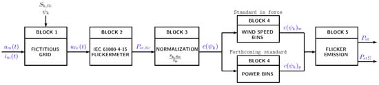
Figure 1.
Block diagram of the measurement and assessment procedure for flicker during continuous operation of a grid connected WT according to the IEC 61400-21 standard in force and its forthcoming edition.
The difference between both procedures lies in the fourth block. The standard in force specifies that each 10 min time series must be classified in wind speed bins according to the mean wind speed. At least 15 10 min time series of voltage and current measurements have to be collected for each 1 m/s wind speed bin, with bins going from a cut-in wind speed of usually 3 m/s to 15 m/s. In contrast, the forthcoming edition of the standard establishes that each 10 min time series has to be classified into power bins, expressed as a percentage of the rated power of the WT, . Moreover, 11 power bins are specified as 0%, 10%, 20%, ⋯, 100% of the , being 0, 10, 20, ⋯, 100 the bin midpoints. In this case, at least 21 10 min time series are required for each power bin.
In Block 1 the interaction between the WT and an ideal grid free from voltage disturbances is implemented through the fictitious grid represented in Figure 2. The WT is modeled by means of a current generator representing the line current measured at the WT terminals. The grid is represented by an ideal voltage generator connected in series with a resistance and an inductance . The ideal voltage has to meet two requirements: it cannot contain any voltage fluctuations, and it shall have the same electrical angle as the voltage measured at the WT terminals []. In this way, the fictitious voltage, , which characterizes the voltage fluctuations produced exclusively by the WT, is obtained according to the following equation:
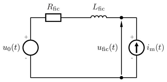
Figure 2.
Fictitious grid implemented in Block 1 of the IEC 61400-21 standard.
The voltage should be obtained for four grid impedance values ( and ), determined by four grid impedance phase angles ( = 30°, 50°, 70° and 85°) and for a specific Short-Circuit Ratio (). The value represents the relation between the short-circuit apparent power of the fictitious grid, , and the rated apparent power of the WT, . The standard specifies a value between 20 and 50. Thus, four voltage signals are obtained for each 10 min time series input at the output of Block 1.
Block 2 implements a class F1 IEC flickermeter according to the IEC 61000-4-15 standard [], obtaining a flicker severity value, , for each voltage. In total, four values are obtained for each 10 min time series, one for each value.
The flicker coefficient is obtained in Block 3 by normalizing the value with the following equation:
According to the standard in force, Block 4 weights the flicker coefficients of the whole set of 10 min time series using four annual average wind speed values. Then, the 99th percentile of each distribution is reported, yielding 16 flicker coefficients . In contrast, the forthcoming edition of the standard would require the 95th percentile of the flicker coefficients for each power bin [], reporting the worst case flicker coefficient for each value.
Based on these reported values, Block 5 estimates the flicker emission from a single WT at the PCC as follows:
where is the grid impedance phase angle at the PCC and is the short-circuit apparent power at the PCC. In case is not one of the values defined by the standard, a linear interpolation of the reported values is suggested to obtain the value.
Finally, the standard determines that the flicker emission of a group of WTs at the PCC could be estimated as follows:
where is the total number of WTs, is the individual flicker coefficient of each WT and the rated apparent power of each WT.
3. Data Collection
This work is based on a large database of real voltage and current waveforms recorded at a 32 MW WPP located in Spain. The WPP is distributed into three strings, comprising a total of 16 Type III 2 MW WTs disposed as shown in Figure 3.
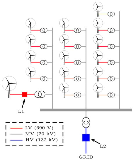
Figure 3.
Illustration of the electrical layout of the WPP.
Each WT is a pitch regulated, upwind WT with active yaw, three-blade rotor, and a high-efficiency 4-pole doubly fed generator with wound rotor and slip rings. The WT has a rated current of 1500 A and 690 V of nominal voltage.
Voltage and current GPS-synchronized measurements were performed at two different locations of the WPP: on the low voltage side (690 V) at the terminals of one WT (L1 in Figure 3), and on the high voltage side (132 kV) at the PCC of the WPP (L2 in Figure 3). During the month and a half long measurement campaign, a total of 4914 10 min time series were recorded at each location. For each time series the operational status of the 16 WTs was annotated and the active power at both locations was calculated. After removing those time series containing switching operations of the WT, and after discarding the time series in which not all the WTs were working, a total number of 3211 10 min time series were selected for the study database. Figure 4a shows the histogram of the time series power at L1, with respect to the of the WT (2 MW), whereas Figure 4b shows the histogram of the time series power at L2, with respect to the of the WPP (32 MW).
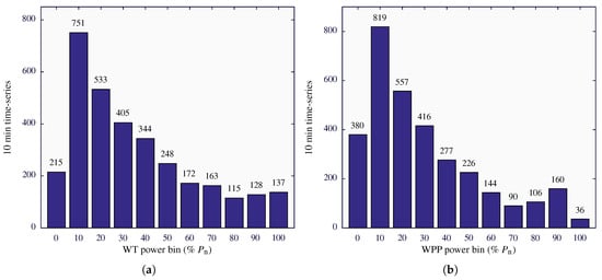
Figure 4.
Power distribution of the selected 10 min time series. (a) Time series recorded at L1 with respect to the power bin of the WT (2 MW). (b) Time series recorded at L2 with respect to the power bin of the WPP (32 MW).
4. Results
Based on the selected 3211 time series, flicker emission values were calculated at the PCC in two ways: first, using the recordings from L1 and following Equation (4); second, using the recordings from L2 and directly calculating the flicker emission. For that purpose, the impedance at the PCC was measured, providing a value of = 6.581∠87.34°. Finally, both results were compared.
4.1. Estimation of the Flicker Emission at the PCC according to IEC 61400-21 Standard
Using the voltage and current time series recorded at L1, the of the WT at the PCC was calculated. To that end, Equation (3) of the IEC 61400-21 procedure was applied, the measured value at the PCC being 2700 MVA. Using these values the flicker summation, , was estimated following Equation (4). This equation can be simplified to , considering that in the selected time series, the 16 WTs were simultaneously working. Figure 5 represents the median, 95th and 99th percentiles of the distribution of values for each . The maximum values were obtained for angles between 40° and 60°. The medians of distributions ranged between 0.0094 and 0.0118. For the particular case of = 87.34°, the complete distribution is represented by means of a boxplot in Figure 5. The edges of the blue box represent the 25th and 75th percentiles, and the black dashed whiskers extend to the minimum and maximum values.
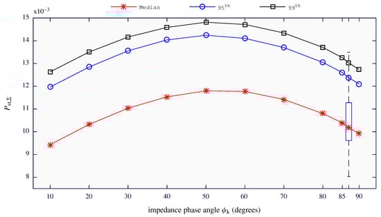
Figure 5.
Statistics of the estimated values at the PCC with respect to the values: median (red asterisks), 95th percentile (blue circles) and 99th percentile (black squares). A boxplot is depicted to represent the distribution for the particular case of = 87.34°.
Figure 6 shows, for the case of = 87.34° and using boxplots, the distribution of values for each power bin of the WT. The central solid horizontal red line in each box is the median and the red crosses represent the outliers of the distributions which were obtained following the Tukey’s fences method []. Black circles represent the 95th percentile for each power bin. According to the standard, these values are those to be reported as the flicker emission for each bin.
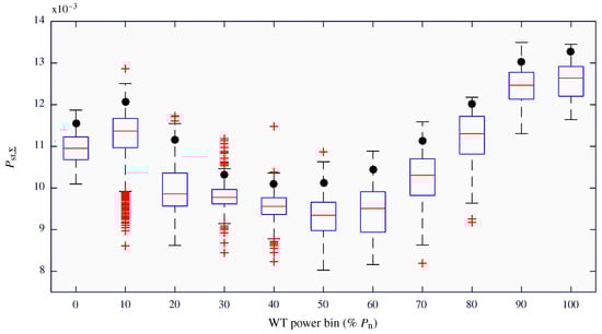
Figure 6.
For a value of 87.34°, boxplots of the estimated values at the PCC with respect to the power bin of the WT (2 MW).
Considering that the registered data was mainly located at the lowest power bins, a greater number of outliers were obtained for those power bins. The lowest values were obtained between the 30% and 60% power bins. For the lowest power bins (0% to 20%) intermediate values were observed. Between the 70% and 100% power bins values increased as the power bin increased. Maximum values were registered between the 90% and 100% power bins. The maximum 95th percentile was 0.0133, obtained for the 100% power bin whose median value is 0.0126.
4.2. Measurement of the Flicker Emission at the PCC
Using the voltage and current time series recorded at L2, the values at the PCC of the WPP were obtained. The direct way to obtain the flicker emission at the PCC is to analyze the registered voltage using the IEC flickermeter. However, this procedure does not distinguish between the flicker emission of the WPP and the background voltage fluctuations present at that measurement point in the grid. Therefore, similarly to what the IEC 61400-21 standard establishes, the flicker emission at the PCC exclusively produced by the WPP was obtained by means of a model representing the interaction between the WPP and the Thevenin’s equivalent circuit of the grid. In this case, the current source represents the current injected by the WPP whose value corresponds to the current registered at L2. For the Thevenin impedance the known value of = 6.581∠87.34° was used.
Figure 7 depicts, the distributions of the measured values for each power bin of the WPP. The obtained values ranged between 0.0033 and 0.0100, showing the low flicker emission level of the WPP. Excluding outliers, the measured values increased as the generated power of the WPP increased from the lowest to the 90% power bin. At this latter power bin, the maximum values were reached. The 100% power bin presented a very low dispersion and lower values compared to the 90% power bin. It is important to note that the 100% power bin represents the situation at which all the WTs of the WPP are working at around the 100% of their power. This implies that the flicker generation of each WT will be practically the same and, therefore, the measured flicker values should be similar.
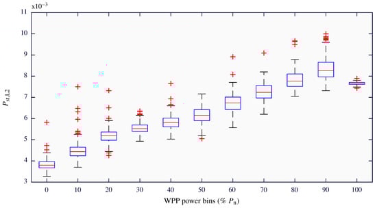
Figure 7.
For a value of 87.34°, boxplots of the measured values at the PCC (16 WTs) with respect to the power bin of the WPP (32 MW).
4.3. Comparison between the Estimated and Measured Flicker Emission at the PCC
The comparison between the estimated and measured values at the PCC was performed using the results obtained for a angle of 87.34°. Overall, the measured values were lower than the estimated ones. This proves that the standard overestimates the flicker emission of the whole WPP.
When comparing the corresponding individual time series at L1 and L2, large deviations were obtained between the measured and estimated flicker emission values. Figure 8a depicts the estimated flicker values versus the measured ones. The results obtained for the time series grouped between the 0% and 30% power bins are represented in black color, whereas the ones corresponding to power bins between 40% and 100% are represented in red. Figure 8b represents, using boxplots, the distributions of the percentage deviation between the estimated and measured values, calculated as:
From left to right, the results correspond to the time series grouped between the 0% to 30%, 40% to 100% and those at the 100% power bin, respectively.
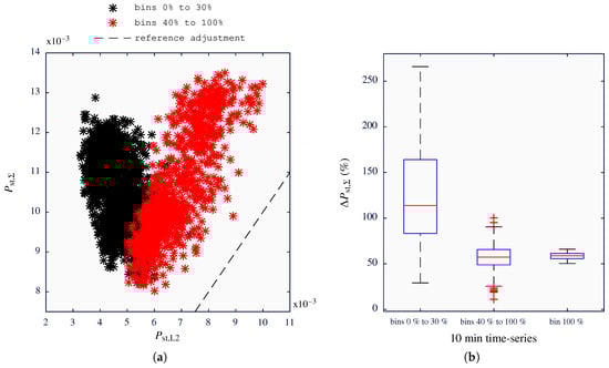
Figure 8.
Deviation between the estimated and measured values at the PCC. (a) Estimated versus measured results, obtained with the time series classified between the power bins 0% to 30% (in black) and between 40% to 100% (in red). (b) Boxplots of the percentage deviation between the estimated and the measured values.
In Figure 8a, two different trends can be distinguished between 0% to 30% and 40% to 100% power bins. Moreover, there is a poor correlation between the obtained results and the dashed black line which represents the ideal situation at which the estimated and measured values are identical. However, if only the time series classified between 40% to 100% power bins are considered, a similar slope is appreciated between the obtained results and the reference values.
Figure 8b shows large deviations between the estimated and measured values. For the particular case of the results obtained for 0% to 30% power bins, half of the deviations were higher than 113%, with a maximum deviation of 265%. On the other hand, for the time series corresponding to power bins between 40% and 100%, half of the deviations were greater than 57%, with a maximum deviation of 100%. Considering only the time series grouped at the 100% power bin, the deviations were concentrated around the 59%, showing a very low dispersion.
The obtained discrepancies may appear for several reasons. On the one hand, the exponent used in the flicker aggregation can make the results be far away from the ideal ones, represented by the dashed black line in Figure 8a. On the other hand, the significant discrepancies obtained for the lowest power bins (0% to 30%) could be the consequence of the existing difficulties in compensating the reactive power when the power generated by the WPP is low [].
4.4. Summation Exponent Effect
When aggregating different flicker sources according to [] an exponent, , is used. The value of depends on the probability of occurrence of coincident fluctuations. Exponents = 1, 2, and 3 represent high, medium, and low probability of occurrence, respectively, whereas = 4 represents very unlikely probability of coincident fluctuations. Currently, the IEC 61400-21 standard in force defines a quadratic summation to estimate the flicker caused by a whole WPP. This is because the WTs are considered stochastic uncorrelated noise sources of flicker, and therefore present a medium probability of occurrence of coincident fluctuations []. However, the effect of the exponent was studied in view of the existing deviations.
The summation exponents providing the estimated values that best fit the measured values, , have been obtained for each time series. Table 1 shows, for each power bin, the median and interquartile range (IQR) of the . The IQR is represented showing the 25th and 75th percentiles in brackets, providing a measure of the dispersion of the values. The median of the exponents ranged between 2.75 and 8.50. For the case of power bins between 0% and 20%, the values presented a larger dispersion than for the rest of the bins. The 100% power bin presented the lowest dispersion. Overall, for the time series grouped in 40% to 100% power bins, the medians of values are within a range of 2.75 and 3.16.

Table 1.
Statistics of the obtained best fitting exponents, , at each power bin of the WPP.
To obtain the value producing the lowest error between the estimated and measured values for the power bins between 40% and 100%, the estimated values were obtained using values between 2 and 4 in steps of 0.1. Figure 9 shows the mean of with respect to the used in the estimation. The time series grouped in the range of 40% to 100% power bins are represented by red circles, and the ones grouped at the 100% power bin by blue asterisks. The lowest mean deviations were given with = 3, for both sets of time series.
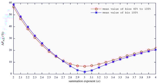
Figure 9.
Mean of percentage deviations between the estimated and measured values with respect to for the time series grouped between the 40% and 100% power bins (red circles), and for the time series grouped at 100% power bin (blue asterisk).
Figure 10 shows the obtained deviations between the estimated and measured flicker values for the case of = 3. There is a better agreement between the estimated and the measured values for the time series grouped between the 40% and 100% power bins. For this set of time series the deviations decreased to less than 10% for the 75% of the values. In the case of the 100% power bin all deviations were below 5%.
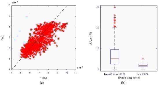
Figure 10.
Deviation between the estimated and measured values at the PCC, for = 3. (a) Estimated versus measured results, obtained with the time series classified between the power bins 40% to 100%. (b) Boxplots of the percentage deviation between the estimated and the measured values.
Finally, the 95th percentile of the measured flicker emission value at the PCC of the WPP was = 0.0082. According to the standard, with = 2, the estimated flicker emission of the WPP at the PCC was = 0.0133, based on the maximum 95th percentile of each power bin. This estimated value presented a deviation of 62% with respect to the measured flicker emission. However, if = 3 is used, an estimated flicker emission of = 0.0084 was obtained, with a deviation of only 2%.
5. Discussion and Conclusions
Technological advances in the wind power sector have reduced considerably the flicker emission of WTs [,,,,]. The implementation of power control methods in modern WTs leads to the reduction of voltage fluctuations [,]. These methods reduce the power fluctuations injected to the grid, and hence also the flicker emission. As an example, the 99th percentile of the flicker coefficients c(85°) reported in [] were 5.8, 3.8 and 2.5 for WTs of types I, II, and IV, respectively. The reduction in flicker emission of these new WTs leads to think about the flicker contribution of a WPP at the PCC. Considering the 32 MW WPP of the study, the 95th percentile of the flicker severity measured on the voltage signal at the PCC was = 0.2572, whereas the 95th percentile of the flicker values emitted exclusively by the WPP at the PCC was only 0.0082. Therefore, this WPP contributes with the 3.19% of the total flicker severity value present at the PCC. The flicker contribution of the WPP in this particular scenario is very low. However, the flicker emission of the WPP depends on the strength of the grid, and in the case of a similar WPP being connected to a weaker grid the flicker emission would be higher. Additionally, a varying number of WPPs can be connected on the same line, affecting the overall flicker contribution.
On the other hand, the IEC 61400-21 standard establishes that the estimation of the flicker emission of a group of WTs can be estimated by means of the quadratic summation of each single flicker value of each WT. The summation exponent = 2 should be used to aggregate flicker sources that present moderate probability of coincident fluctuations []. All the studies that helped to define the standard, and those that later corroborated its validity, were based on measurements carried out at type I or II WTs. However, the results obtained in this work suggest that the flicker aggregation in a WPP with type III WTs should not be quadratic, but cubic. Type I and II WTs present a flicker emission characteristic directly related to the wind speed: power fluctuations caused by variations in the wind speed, are the ones producing flicker emission. Understandably, the effect of the wind is similar in WTs situated in nearby locations, presenting a moderate probability of generating coincident fluctuations between the WTs. However, type III and IV WTs implement power control systems based on power electronics, which manage the total or partial power injection into the grid. Such power management systems minimize the direct effect of wind fluctuations on the generated power. In fact, the flicker emission characteristic of these types of WTs remains almost constant regardless of the wind speed. Therefore, it seems also reasonable that with these types of WTs the probability of presenting coincident fluctuations is lower than with type I or II WTs. According to [], an exponent of 3 should be used to aggregate flicker sources with low probability of coincident fluctuations. Moreover, = 3 is the exponent proposed by the IEC 61000-3-7 standard for general use when additional information is not available to justify a different value.
More studies covering different configurations of WPPs with different types of WTs are needed to confirm the results of this work. In any case, a revision of the flicker summation law currently proposed by the standard is warranted.
Author Contributions
K.R. has performed the experimental activity and the data processing; J.J.G. has contributed in the conceptualization of the study; K.R., J.J.G., I.A., P.S. and L.A.L. have carried out the data acquisition in the WPP; K.R. and I.A. have prepared the first draft of the manuscript; J.J.G., I.A., P.S. and S.R.d.G. have reviewed and edited the manuscript. All the authors have approved the submitted version of this manuscript.
Funding
This research was funded by Basque Government (Basque Country, Spain) through the project IT1087-16 and by the Spanish MINECO through project DPI2014-53317-R (co-financed with European FEDER funds).
Conflicts of Interest
The authors declare no conflict of interest.
Abbreviations
The following abbreviations are used in this manuscript:
| GPS | Global Positioning System |
| IEC | International Electrotechnical Commission |
| IQR | Interquartile range |
| PCC | Point of Common Coupling |
| PQ | Power Quality |
| Short-Circuit Ratio | |
| WPP | Wind Power Plant |
| WT | Wind Turbine |
References
- GWEC (Global Wind Energy Council). Global Wind Report—Annual Market Update 2017; Technical Report; Global Wind Energy Council: Brussels, Belgium, 2018. [Google Scholar]
- GWEC (Global Wind Energy Council). Global Wind Energy Outlook 2016; Technical Report; Global Wind Energy Council: Brussels, Belgium, 2016. [Google Scholar]
- Liang, X. Emerging Power Quality Challenges Due to Integration of Renewable Energy Sources. IEEE Trans. Ind. Appl. 2017, 53, 855–866. [Google Scholar] [CrossRef]
- IEC (International Electrotechnical Commission). Wind Turbines—Part 21: Measurement and Assesment of Power Quality Characteristics of Grid Connected Wind Turbines, 2nd ed.; IEC 61400-21; IEC: Geneva, Switzerland, 2008. [Google Scholar]
- Abubakar, U.; Mekhilef, S.; Mokhlis, H.; Seyedmahmoudian, M.; Horan, B.; Stojcevski, A.; Bassi, H.; Hosin Rawa, M.J. Transient Faults in Wind Energy Conversion Systems: Analysis, Modelling Methodologies and Remedies. Energies 2018, 11, 2249. [Google Scholar] [CrossRef]
- García, H.; Segundo, J.; Rodríguez-Hernández, O.; Campos-Amezcua, R.; Jaramillo, O. Harmonic Modelling of the Wind Turbine Induction Generator for Dynamic Analysis of Power Quality. Energies 2018, 11, 104. [Google Scholar] [CrossRef]
- Sellami, T.; Berriri, H.; Jelassi, S.; Darcherif, A.M.; Mimouni, M.F. Short-Circuit Fault Tolerant Control of a Wind Turbine Driven Induction Generator Based on Sliding Mode Observers. Energies 2017, 10, 1611. [Google Scholar] [CrossRef]
- IEC (International Electrotechnical Commission). Wind Turbine Generator Systems—Part 21: Measurement and Assessment of Power Quality Characteristics of Grid Connected Wind Turbines, 1st ed.; IEC 61400-21; IEC: Geneva, Switzerland, 2001. [Google Scholar]
- Sorensen, P.; Tande, J.O.; Sondergaard, L.; Kledal, J.D. Flicker Emission Levels from Wind Turbines. Wind Eng. 1996, 20, 39–46. [Google Scholar]
- Larsson, A. Flicker emission of wind turbines during continuous operation. IEEE Trans. Energy Convers. 2002, 17, 114–118. [Google Scholar] [CrossRef]
- Barahona, B.; Sorensen, P.; Christensen, L.; Sorensen, T.; Nielsen, H.; Larsen, X. Validation of the Standard Method for Assessing Flicker From Wind Turbines. IEEE Trans. Energy Convers. 2011, 26, 373–378. [Google Scholar] [CrossRef]
- Christensen, L.; Sorensen, P.; Sorensen, T.S.; Nielsen, H. Evaluation of Measuring Methods for Flicker Emission from Modern Wind Turbine; AEE: Madrid, Spain, 2009. [Google Scholar]
- Ammar, M.; Joos, G. Impact of Distributed Wind Generators Reactive Power Behavior on Flicker Severity. IEEE Trans. Energy Convers. 2013, 28, 425–433. [Google Scholar] [CrossRef]
- Chen, Z.; Guerrero, J.; Blaabjerg, F. A Review of the State of the Art of Power Electronics for Wind Turbines. IEEE Trans. Power Electron. 2009, 24, 1859–1875. [Google Scholar] [CrossRef]
- IEC (International Electrotechnical Commission). Electromagnetic Compatibility (EMC)—Part 3–7: Limits–Assessment of Emission limits for the Connection of Fluctuating Installations to MV, HV and EHV Power Systems, 2nd ed.; IEC/TR 61000-3-7; IEC: Geneva, Switzerland, 2008. [Google Scholar]
- Sorensen, P.; Pedersen, T.F.; Gerdes, G.; Klosse, R.; Santjer, F.; Robertson, N.; Davy, W.; Koulouvari, M.; Morfiadakis, E.; Larsson, A. European Wind Turbine Testing Procedure Developments Task 2: Power Quality; Technical Report; Riso National Laboratory: Roskilde, Denmark, 2001. [Google Scholar]
- Sorensen, P. Methods for Calculation of the Flicker Contributions from Wind Turbines; Technical Report Riso-I-939(EN); Riso National Laboratory: Roskilde, Denmark, 1995. [Google Scholar]
- Thiringer, T.; Petru, T.; Lundberg, S. Flicker Contribution from Wind Turbine Installations. IEEE Trans. Energy Convers. 2004, 19, 157–163. [Google Scholar] [CrossRef]
- Andresen, B.; Sørensen, P.; Santjer, F.; Niiranen, J. Overview, status and outline of the new revision for the IEC 61400-21—Measurement and assessment of power quality characteristics of grid connected wind turbines. In 12th International Workshop on Large-Scale Integration of Wind Power into Power Systems as well as on Transmission Networks for Offshore Wind Power Plants; Energynautics GmbH: Darmstadt, Germany, 2013. [Google Scholar]
- Redondo, K.; Lazkano, A.; Saiz, P.; Gutierrez, J.J.; Azcarate, I.; Leturiondo, L.A. A strategy for improving the accuracy of flicker emission measurement from wind turbines. Electr. Power Syst. Res. 2016, 133, 12–19. [Google Scholar] [CrossRef]
- IEC (International Electrotechnical Commission). Electromagnetic Compatibility (EMC)—Part 4: Testing and Measurements Techniques—Section 15: Flickermeter Functional and Desing Specifications, 2nd ed.; IEC 61000-4-15; IEC: Geneva, Switzerland, 2010. [Google Scholar]
- Lazkano, A.; Redondo, K.; Gutierrez, J.; Saiz, P.; Leturiondo, L.; Azkarate, I. Revision of the standard method for statistical evaluation of flicker coefficients in wind turbines. In Proceedings of the 2014 IEEE 16th International Conference on Harmonics and Quality of Power (ICHQP), Bucharest, Romania, 25–28 May 2014; pp. 258–262. [Google Scholar] [CrossRef]
- Tukey, J.W. Exploratory Data Analysis; Addison-Wesley Series in Behavioral Science: Quantitative Methods; Addison-Wesley: Boston, MA, USA, 1977. [Google Scholar]
- Camm, E.H.; Behnke, M.R.; Bolado, O.; Bollen, M.; Bradt, M.; Brooks, C.; Dilling, W.; Edds, M.; Hejdak, W.J.; Houseman, D.; et al. Reactive power compensation for wind power plants. In Proceedings of the 2009 IEEE Power Energy Society General Meeting, Calgary, AB, Canada, 26–30 July 2009; pp. 1–7. [Google Scholar] [CrossRef]
- She, X.; Huang, A.; Wang, F.; Burgos, R. Wind Energy System With Integrated Functions of Active Power Transfer, Reactive Power Compensation, and Voltage Conversion. IEEE Trans. Ind. Electron. 2013, 60, 4512–4524. [Google Scholar] [CrossRef]
© 2019 by the authors. Licensee MDPI, Basel, Switzerland. This article is an open access article distributed under the terms and conditions of the Creative Commons Attribution (CC BY) license (http://creativecommons.org/licenses/by/4.0/).