Condition Monitoring of Bearing Faults Using the Stator Current and Shrinkage Methods

 ,
,  ,
,  and
and
Abstract
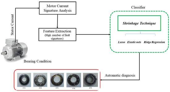
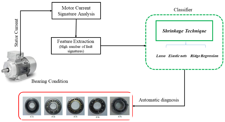
1. Introduction
2. Fault Signatures
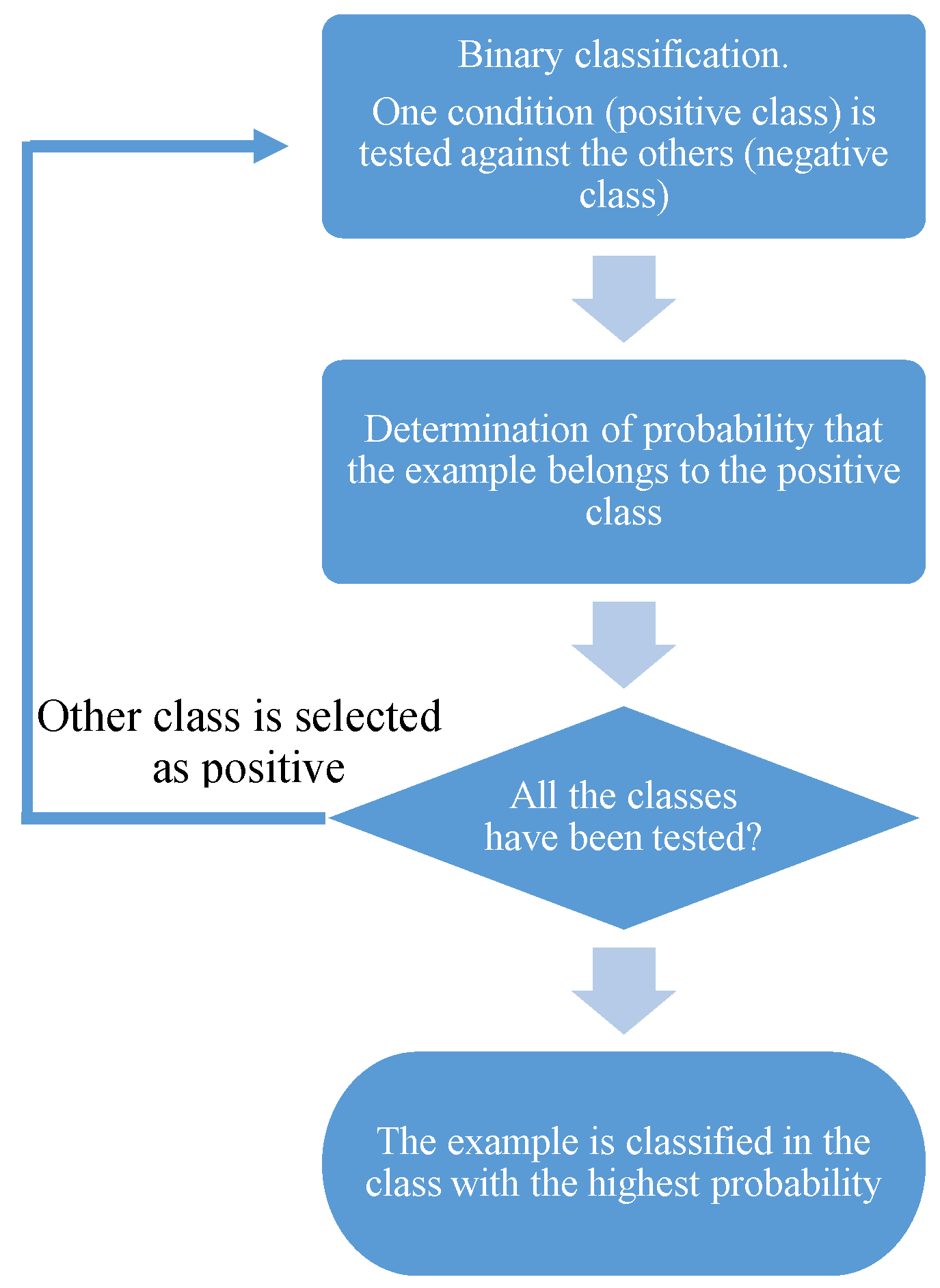
3. Diagnosis
4. Results
4.1. Test Bench
4.2. Classification with 968 Fault Signatures
4.3. Classification with 968 Fault Signatures by Applying Shrinkage
5. Discussion
Author Contributions
Funding
Conflicts of Interest
References
- Immovilli, F.; Bellini, A.; Rubini, R.; Tassoni, C. Diagnosis of bearing faults in induction machines by vibration or current signals: A critical comparison. IEEE Trans. Ind. Appl. 2010, 46, 1350–1359. [Google Scholar] [CrossRef]
- Henao, H.; Capolino, G.A.; Fernandez-Cabanas, M.; Filippetti, F.; Bruzzese, C.; Strangas, E.; Pusca, R.; Estima, J.; Riera-Guasp, M.; Hedayati-Kia, S. Trends in fault diagnosis for electrical machines. IEEE Ind. Electron. Mag. 2014, 8, 31–42. [Google Scholar] [CrossRef]
- Akin, B.; Toliyat, H.A.; Orguner, U.; Rayner, M. PWM Inverter Harmonics Contributions to the Inverter-Fed Induction Machine Bearing Fault Diagnosis. In Proceedings of the IEEE Applied Power Electronics Conference, APEC 2007—Twenty Second Annual, Anaheim, CA, USA, 25 February–1 March 2007; pp. 1393–1399. [Google Scholar]
- Bellini, A.; Filippetti, F.; Tassoni, C.; Capolino, G.-A. Advances in diagnostic techniques for induction machines. IEEE Trans. Ind. Electron. 2008, 55, 4109–4126. [Google Scholar] [CrossRef]
- Zarei, J.; Poshtan, J. An advanced Park’s vectors approach for bearing fault detection. Tribol. Int. 2009, 42, 213–219. [Google Scholar] [CrossRef]
- Blodt, M.; Granjon, P.; Raison, B.; Rostaing, G. Models for bearing damage detection in induction motors using stator current monitoring. IEEE Trans. Ind. Electron. 2008, 55, 1813–1822. [Google Scholar] [CrossRef]
- Duque, O.; Pérez, M.; Moríñigo, D. Detection of bearing faults in cage induction motors fed by frequency converter using spectral analysis of line current. In Proceedings of the IEEE International Conference on Electric Machines and Drives, San Antonio, TX, USA, 15 May 2005; pp. 17–22. [Google Scholar]
- Zhou, W.; Habetler, T.G.; Harley, R.G. Bearing Fault Detection Via Stator Current Noise Cancellation and Statistical Control. IEEE Trans. Ind. Electron. 2008, 55, 4260–4269. [Google Scholar] [CrossRef]
- Singh, S.; Kumar, A.; Kumar, N. Motor Current Signature Analysis for Bearing Fault Detection in Mechanical Systems. Procedia Mater. Sci. 2014, 6, 171–177. [Google Scholar] [CrossRef]
- Deekshit Kompella, K.C.; Venu Gopala Rao, M.; Srinivasa Rao, R. DWT based bearing fault detection in induction motor using noise cancellation. J. Electr. Syst. Inf. Technol. 2016, 3, 411–427. [Google Scholar]
- Rosero, J.; Cusido, J.; Garcia Espinosa, A.; Ortega, J.A.; Romeral, L. Broken Bearings Fault Detection for a Permanent Magnet Synchronous Motor under non-constant working conditions by means of a Joint Time Frequency Analysis. In Proceedings of the IEEE International Symposium on Industrial Electronics, Vigo, Spain, 4–7 June 2007; pp. 3415–3419. [Google Scholar]
- Kablaa, A.; Mokrani, K. Bearing fault diagnosis using Hilbert-Huang transform (HHT) and support vector machine (SVM). Mech. Ind. 2016, 17, 308. [Google Scholar] [CrossRef]
- Elbouchikhi, E.; Choqueuse, V.; Amirat, Y.; Benbouzid, M.E.H.; Turri, S. An Efficient Hilbert-Huang Transform-Based Bearing Faults Detection in Induction Machines. IEEE Trans. Energy Convers. 2017, 32, 401–413. [Google Scholar] [CrossRef]
- Camarena-Martinez, D.; Osornio-Rios, R.; Romero-Troncoso, R.J.; Garcia-Perez, A. Fused Empirical Mode Decomposition and MUSIC Algorithms for Detecting Multiple Combined Faults in Induction Motors. J. Appl. Res. Technol. 2015, 13, 160–167. [Google Scholar] [CrossRef]
- Amirata, Y.; Benbouzidb, M.E.H.; Wang, T.; Bachad, K.; Felda, G. EEMD-based notch filter for induction machine bearing faults detection. Appl. Acous. 2018, 133, 202–209. [Google Scholar] [CrossRef]
- Alwodai, A.; Wang, T.; Chen, Z.; Gu, F.; Cattley, R.; Ball, A. A Study of Motor Bearing Fault Diagnosis using Modulation Signal Bispectrum Analysis of Motor Current Signals. J. Sign. and Inform. Proc. 2013, 4, 72–79. [Google Scholar] [CrossRef]
- Leite, V.C.M.N.; Borges da Silva, J.G.; Veloso, G.F.C.; Borges da Silva, L.E.; Lambert-Torres, G.; Bonaldi, E.L.; de Oliveira, L.E.L. Detection of Localized Bearing Faults in Induction Machines by Spectral Kurtosis and Envelope Analysis of Stator Current. IEEE Trans. Ind. Electron. 2015, 62, 1855–1865. [Google Scholar] [CrossRef]
- El Bouchikhi, E.H.; Choqueuse, V.; Benbouzid, M.E.H. Current Frequency Spectral Subtraction and Its Contribution to Induction Machines’ Bearings Condition Monitoring. IEEE Trans. Energy Convers. 2013, 28, 135–144. [Google Scholar] [CrossRef]
- Arkan, M.; Çaliş, H.; Tağluk, M.E. Bearing and misalignment fault detection in induction motors by using the space vector angular fluctuation signal. Electr. Eng. 2005, 87, 197–206. [Google Scholar] [CrossRef]
- Boudinar, A.H.; Benouzza, N.; Bendiabdellah, A.; Khodja, A. Induction Motor Bearing Fault Analysis Using a Root-MUSIC Method. IEEE Trans. Ind. Appl. 2016, 52, 3851–3860. [Google Scholar] [CrossRef]
- El Bouchikhi, E.H.; Choqueuse, V.; Benbouzid, M.E.H. Induction machine bearing faults detection based on a multi-dimensional MUSIC algorithm and maximum likelihood estimation. ISA Trans. 2016, 63, 413–424. [Google Scholar] [CrossRef]
- Godoy, W.F.; da Silva, I.N.; Goedtel, A.; Palácios, R.H.C.; Gongora, W.S. Neural approach for bearing fault classification in induction motors by using motor current and voltage. In Proceedings of the IEEE International Joint Conference on Neural Networks (IJCNN), Beijing, China, 6–11 July 2014; pp. 2087–2092. [Google Scholar]
- Ballal, M.S.; Khan, Z.J.; Suryawanshi, H.M.; Sonolikar, R.L. Adaptive Neural Fuzzy Inference System for the Detection of Inter-Turn Insulation and Bearing Wear Faults in Induction Motor. IEEE Trans. Ind. Electron. 2007, 54, 250–258. [Google Scholar] [CrossRef]
- Zarei, J.; Arefi, M.M.; Hassani, H. Bearing fault detection based on interval type-2 fuzzy logic systems for support vector machines. In Proceedings of the 6th International Conference on Modeling, Simulation and Applied Optimization (ICMSAO), Istanbul, Turkey, 27–29 May 2015; pp. 1–6. [Google Scholar]
- Salem, S.B.; Bacha, K.; Chaari, A. Support vector machine based decision for mechanical fault condition monitoring in induction motor using an advanced Hilbert-Park transform. ISA Trans. 2012, 51–55, 566–572. [Google Scholar] [CrossRef]
- Bouguerne, A.; Lebaroud, A.; Medoued, A.; Boukadoum, A. Classification of induction machine faults by K-nearest neighbor. In Proceedings of the 7th International Conference on Electrical and Electronics Engineering (ELECO), Bursa, Turkey, 1–4 December 2011; pp. I-363–I-366. [Google Scholar]
- Tian, J.; Morillo, C.; Azarian, M.H.; Pecht, M. Motor Bearing Fault Detection Using Spectral Kurtosis-Based Feature Extraction Coupled with K-Nearest Neighbor Distance Analysis. IEEE Trans. Ind. Electron. 2016, 63, 1793–1803. [Google Scholar] [CrossRef]
- Farajzadeh-Zanjani, M.; Razavi-Far, R.; Saif, M. Diagnosis of Bearing Defects in Induction Motors by Fuzzy-Neighborhood Density-Based Clustering. In Proceedings of the IEEE 14th International Conference on Machine Learning and Applications, Miami, FL, USA, 9–11 December 2015; pp. 935–940. [Google Scholar]
- Peng, H.-W.; Chiang, P.-J. Control of mechatronics systems: Ball bearing fault diagnosis using machine learning techniques. In Proceedings of the 8th Asian Control Conference (ASCC), Kaohsiung, Taiwan, 15–18 May 2011; pp. 175–180. [Google Scholar]
- Santos, S.P.; Costa, J.A.F. A Comparison between Hybrid and Non-hybrid Classifiers in Diagnosis of Induction Motor Faults. In Proceedings of the 11th IEEE International Conference on Computational Science and Engineering, Sao Paulo, Brazil, 16–18 July 2008; pp. 301–306. [Google Scholar]
- Ergin, S.; Tezel, S.; Gulmezoglu, M.B. DWT-based fault diagnosis in induction motors by using CVA. In Proceedings of the International Symposium on Innovations in Intelligent Systems and Applications (INISTA), Istanbul, Turkey, 15–18 June 2011; pp. 129–132. [Google Scholar]
- Cunha Palácios, R.H.; da Silva, I.N.; Goedtel, A.; Godoy, W.F. A comprehensive evaluation of intelligent classifiers for fault identification in three-phase induction motors. Electr. Power Syst. Res. 2015, 127, 249–258. [Google Scholar] [CrossRef]
- Sugumaran, V.; Ramachandran, K.I. Automatic rule learning using decision tree for fuzzy classifier in fault diagnosis of roller bearing. Mech. Syst. Signal Process. 2007, 21, 2237–2247. [Google Scholar] [CrossRef]
- Zeng, M.; Yang, Y.; Zheng, J.; Cheng, J. Maximum margin classification based on flexible convex hulls for fault diagnosis of roller bearings. Mech. Syst. Signal Process. 2016, 66–67, 533–545. [Google Scholar] [CrossRef]
- Mbo’o, C.P.; Hameyer, K. Fault Diagnosis of Bearing Damage by Means of the Linear Discriminant Analysis of Stator Current Features from the Frequency Selection. IEEE Trans. Ind. Appl. 2016, 52, 3861–3868. [Google Scholar]
- Montechiesi, L.; Cocconcelli, M.; Rubini, R. Artificial immune system via Euclidean Distance Minimization for anomaly detection in bearings. Mech. Syst. Signal Process. 2016, 76, 380–393. [Google Scholar] [CrossRef]
- Wang, D. An extension of the infograms to novel Bayesian inference for bearing fault feature identification. Mech. Syst. Signal Process. 2016, 80, 19–30. [Google Scholar] [CrossRef]
- Frosini, L.; Bassi, E.; Fazzi, A.; Gazzaniga, C. Use of the stator current for condition monitoring of bearings in induction motors. In Proceedings of the 2008 International Conference on Electrical Machines, Vilamoura, Portugal, 6–9 September 2008; pp. 1–6. [Google Scholar]
- Morinigo-Sotelo, D.; Duque-Perez, O.; Perez-Alonso, M. Assessment of the lubrication condition of a bearing using spectral analysis of the stator current. In Proceedings of the International Symposium on Power Electronics Electrical Drives Automation and Motion (SPEEDAM), Pisa, Italy, 14–16 June 2010; pp. 1160–1165. [Google Scholar]
- Domingos, P. The Master Algorithm; Basic Books: New York, NY, USA, 2015. [Google Scholar]
- Benbouzid, M.E.H.; Kliman, G.B. What stator current processing based technique to use for induction motor rotor faults diagnosis? IEEE Trans. Energy Convers. 2003, 18, 238–244. [Google Scholar] [CrossRef]
- James, G.; Witten, D.; Tibshirani, T.H.R. An Introduction to Statistical Learning; Springer: Berlin, Germany, 2013. [Google Scholar]
- Amaral Santos, P.L.; Imangaliyev, S.; Schutte, K.; Levin, E. Feature selection via co-regularized sparse-group Lasso. In Machine Learning, Optimization and Big Data; Pardalos, P.M., Conca, P., Giuffrida, G., Nicosi, G., Eds.; Springer: Berlin, Germany, 2016; pp. 118–131. [Google Scholar]
- Tibshirani, D.R. Regression shrinkage and selection via the lasso: A retrospective. J. R. Statist. Soc. B 2011, 73, 273–282. [Google Scholar] [CrossRef]
- Zhang, X. Regularization. In Encyclopedia of Machine Learning, 2010 ed.; Sammut, C., Webb, G.I., Eds.; Springer: Boston, MA, USA, 2010. [Google Scholar]
- Kleinbaum, G.; Klein, M. Logistic Regression, 3rd ed.; Spinger Science+Business Media: New York, NY, USA, 2010. [Google Scholar]
- Pampel, F.C. Logistic Regression. A Primer; Sage Publications: Thousand Oaks, CA, USA, 2000. [Google Scholar]


| Traditional Approach | Proposed Approach | |
|---|---|---|
| Bearing fault frequencies | BPFO 1, BPFI 2, FTF 3; BSF 4 | BPFO 1, BPFI 2, FTF 3; BSF 4 |
| Harmonics considered | 1 | 1, 2, …, 11 |
| Sidebands around harmonic | 1 | 1, 2, …, 11 |
| Number of fault signatures | 8 | 968 |
| Supply Identification | Power Source | Operating Frequency | Switching Frequency |
|---|---|---|---|
| S1 | utility | 50 Hz | - |
| S2 | Power converter | 50 Hz | 4 kHz |
| S3 | Power converter | 25 Hz | 4 kHz |
| S4 | Power converter | 50 Hz | 5 kHz |
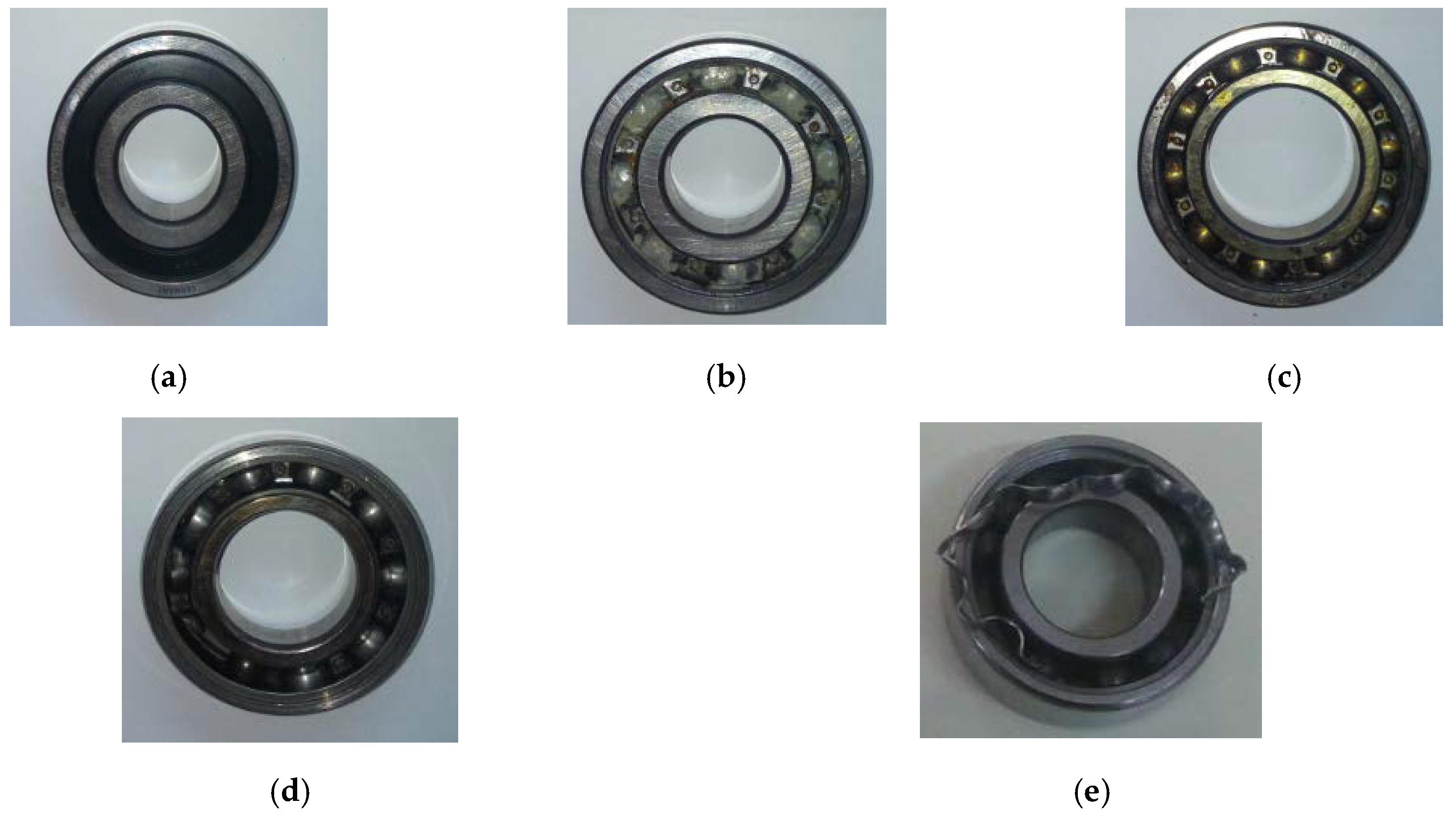
| Condition | Evolution of the Fault | Number of Tests Per Supply |
|---|---|---|
| C1 | healthy state | 20 |
| C2 | incipient fault | 15 |
| C3 | intermediate fault | 15 |
| C4 | developed fault | 10 |
| C5 | complete breakdown | 10 |
| Supply Identification | Load | Best Accuracy 968 Fault Signatures | Best Algorithm 968 Fault Signatures | Best Accuracy 8 Fault Signatures | Best Algorithm 8 Fault Signatures |
|---|---|---|---|---|---|
| S1 | Low | 95.7% | KNN 1 | 40% | SVM 2 |
| High | 92.9% | SVM 2 | 40% | SVM 2 | |
| S2 | Low | 88.6% | SVM 2 | 32.9% | BT 5 |
| High | 98.6% | SVM 2 | 44.3% | BT 5 | |
| S3 | Low | 81.4% | BT 5 | 41.4% | SVM 2 |
| High | 97.1% | LD 4 | 60% | KNN 1 | |
| S4 | Low | 85.7% | LD 4 | 41.4% | SVM 2 |
| High | 98.6% | BT 5 | 42.9% | SVM 2 |
| Supply Identification | Load | Lasso | Elastic Nets | Ridge Regression |
|---|---|---|---|---|
| S1 | Low | 100 | 100 | 100 |
| High | 90.48 | 90.48 | 85.71 | |
| S2 | Low | 95.24 | 90.48 | 80.95 |
| High | 95.24 | 100 | 100 | |
| S3 | Low | 80.95 | 76.19 | 76.19 |
| High | 90.48 | 95.24 | 95.24 | |
| S4 | Low | 90.48 | 80.95 | 85.71 |
| High | 100 | 95.24 | 85.71 |
| Supply | Load | Regularization Parameter |
|---|---|---|
| S1 | High | 0.02 |
| Low | 0.05 | |
| S2 | High | 0.0003 |
| Low | 0.02 | |
| S3 | High | 0.01 |
| Low | 0.01 | |
| S4 | High | 0.005 |
| Low | 0.005 |
| Low Load | High Load | ||||||||||
|---|---|---|---|---|---|---|---|---|---|---|---|
| Predicted Class | Predicted Class | ||||||||||
| True class | C1 | C2 | C3 | C4 | C5 | C1 | C2 | C3 | C4 | C5 | |
| C1 | 6 | 0 | 0 | 0 | 0 | 6 | 0 | 0 | 0 | 0 | |
| C2 | 0 | 5 | 0 | 0 | 0 | 0 | 3 | 0 | 0 | 1 | |
| C3 | 0 | 0 | 4 | 0 | 0 | 0 | 1 | 4 | 0 | 0 | |
| C4 | 0 | 0 | 0 | 3 | 0 | 0 | 0 | 0 | 3 | 0 | |
| C5 | 0 | 0 | 0 | 0 | 3 | 0 | 0 | 0 | 0 | 3 | |
| Low Load | High Load | ||||||||||
|---|---|---|---|---|---|---|---|---|---|---|---|
| Predicted Class | Predicted Class | ||||||||||
| True class | C1 | C2 | C3 | C4 | C5 | C1 | C2 | C3 | C4 | C5 | |
| C1 | 6 | 0 | 0 | 0 | 0 | 6 | 0 | 0 | 0 | 0 | |
| C2 | 1 | 3 | 0 | 0 | 0 | 0 | 3 | 0 | 0 | 1 | |
| C3 | 0 | 0 | 5 | 0 | 0 | 0 | 1 | 4 | 0 | 0 | |
| C4 | 0 | 0 | 0 | 3 | 0 | 0 | 0 | 0 | 3 | 0 | |
| C5 | 0 | 0 | 0 | 0 | 3 | 0 | 0 | 0 | 0 | 3 | |
| Low Load | High Load | ||||||||||
|---|---|---|---|---|---|---|---|---|---|---|---|
| Predicted Class | Predicted Class | ||||||||||
| True class | C1 | C2 | C3 | C4 | C5 | C1 | C2 | C3 | C4 | C5 | |
| C1 | 5 | 1 | 0 | 0 | 0 | 6 | 0 | 0 | 0 | 0 | |
| C2 | 0 | 4 | 0 | 0 | 0 | 0 | 4 | 0 | 0 | 0 | |
| C3 | 0 | 0 | 3 | 1 | 1 | 1 | 1 | 3 | 0 | 0 | |
| C4 | 0 | 0 | 0 | 3 | 0 | 0 | 0 | 0 | 3 | 0 | |
| C5 | 0 | 0 | 0 | 1 | 2 | 0 | 0 | 0 | 0 | 3 | |
| Low Load | High Load | ||||||||||
|---|---|---|---|---|---|---|---|---|---|---|---|
| Predicted Class | Predicted Class | ||||||||||
| True class | C1 | C2 | C3 | C4 | C5 | C1 | C2 | C3 | C4 | C5 | |
| C1 | 6 | 0 | 0 | 0 | 0 | 6 | 0 | 0 | 0 | 0 | |
| C2 | 0 | 4 | 0 | 0 | 0 | 0 | 4 | 0 | 0 | 0 | |
| C3 | 0 | 0 | 4 | 0 | 1 | 0 | 0 | 5 | 0 | 0 | |
| C4 | 0 | 0 | 1 | 2 | 0 | 0 | 0 | 0 | 3 | 0 | |
| C5 | 0 | 0 | 0 | 0 | 3 | 0 | 0 | 0 | 0 | 3 | |
© 2019 by the authors. Licensee MDPI, Basel, Switzerland. This article is an open access article distributed under the terms and conditions of the Creative Commons Attribution (CC BY) license (http://creativecommons.org/licenses/by/4.0/).
Share and Cite
Duque-Perez, O.; Del Pozo-Gallego, C.; Morinigo-Sotelo, D.; Fontes Godoy, W. Condition Monitoring of Bearing Faults Using the Stator Current and Shrinkage Methods. Energies 2019, 12, 3392. https://doi.org/10.3390/en12173392
Duque-Perez O, Del Pozo-Gallego C, Morinigo-Sotelo D, Fontes Godoy W. Condition Monitoring of Bearing Faults Using the Stator Current and Shrinkage Methods. Energies. 2019; 12(17):3392. https://doi.org/10.3390/en12173392
Chicago/Turabian StyleDuque-Perez, Oscar, Carlos Del Pozo-Gallego, Daniel Morinigo-Sotelo, and Wagner Fontes Godoy. 2019. "Condition Monitoring of Bearing Faults Using the Stator Current and Shrinkage Methods" Energies 12, no. 17: 3392. https://doi.org/10.3390/en12173392
APA StyleDuque-Perez, O., Del Pozo-Gallego, C., Morinigo-Sotelo, D., & Fontes Godoy, W. (2019). Condition Monitoring of Bearing Faults Using the Stator Current and Shrinkage Methods. Energies, 12(17), 3392. https://doi.org/10.3390/en12173392