Decision Making using Logical Decision Tree and Binary Decision Diagrams: A Real Case Study of Wind Turbine Manufacturing

Abstract

The wind energy industry is expanding in order to be able to meet the current and future energy demand, and is supported by governments in that renewable energy investment has been made. Optimal decision making (DM) in wind turbine manufacturing is required to guarantee the competitiveness of the business. This paper considers decision making for wind turbine manufacturing using a logical decision tree (LDT) and binary decision diagrams (BDD). A qualitative analysis of wind turbine manufacturing is carried out using logical decision trees. They are used for a qualitative study of the case study. Binary decision diagrams are used to obtain the Boolean function and, therefore, to carry out a quantitative analysis. Finally, an optimization of budgets is employed based on importance measures. There is no optimal method that can establish the importance measures. The following heuristic methods have been used to find a solution close to the optimal: Fussell-Vesely, Birnbaum and Criticality. The computational cost is reduced by ranking the events. The heuristic methods to establish the best rankings are: Top-Down-Left-Right, Level based method, AND based method, Breadth-First Search (BFS) and Depth First Search (DFS). A real case study is considered, in which a static and dynamic analysis is carried out.

1. Introduction

Wind energy has been growing in recent years. Forecasting studies confirm that it will continue to increase until at least 2030. Wind farms require an acceptable level of reliability, availability, maintainability and safety (RAMS) of wind turbines in order to guarantee power generation levels that contribute to the energy mix [1,2].

Vachon [3] shows that operations and maintenance (OM) costs can make up 75–90% of the investment costs, based on a 20-year life cycle for a 100-MW wind farm with 600 turbines of 750 kW each. The cost per failure is increasing, although larger turbines may reduce the OM cost per unit power [4]. Therefore, the correct decision making (DM) in design, manufacture and performance of wind turbines must be set correctly. This will mean that operational and maintenance costs and downtimes can be minimized or avoided [5,6]. Figure 1 shows the principal components of a wind turbine [7].

There are several research studies that consider the wind turbine manufacturing process: Han et al. [8] presented the manufacture of a 100-W helical-blade vertical-axis wind turbine. The manufacture was optimized by numerical analysis in the design process, and it was tested in a wind tunnel. Wind turbine manufacturing is optimized to achieve competitiveness in the market. Therefore, a correct and optimal DM is required in wind turbine manufacturing. Pérez et al. [7] considered a complete analysis of wind turbine reliability, which depends on the correct manufacture in terms of the components studied. Márquez et al. [9] took into account the critical components via fault tree analysis over time, concluding that these components should be considered in detail in the production phase. A similar research study was carried out for electrical components by García et al. [10]. Pérez et al. [4] studied the critical components from an economic perspective, in which the investment costs of the manufacturing process were considered. Dale et al. [11] presented a dynamic function for energy return on investments, which is mainly due to the manufacturing process. Coudert and Madre presented presents data structures and algorithms that support the interactive exact analysis of very large coherent and noncoherent fault trees [12]. None of these studies considers the DM in the manufacturing process, but it can be found in other fields. The DM problem has been considered from different perspectives: Cost-benefit-cost study; basic rules [13], e.g., conjunctive and disjunctive, maximin and maximax, lexicographic, pros and cons analysis; analytic hierarchy process generalized means, simple multi-attribute rating, outranking; the fuzzy preference relations [14]; cognitive decision–making models [15]; large group DM methods [16,17]; ELECTRE and PROMETHEE [13]; etc.

New researches have been conducted in DM processes under risk contexts, e.g., References [18,19,20]. These methods solve the problem usually from a quantitative perspective, and sometimes from a qualitative one, but they do not consider both together.

This paper considers an approach to DM problem analysis from qualitative and quantitative perspectives, i.e., graphically and mathematically, where they are linked. The paper discusses the logical decision tree (LDT) to support these decisions for optimal, or close to optimal, wind turbine manufacturing. The LDT leads a DM qualitative analysis. The LDT is converted to binary decision diagrams (BDD). The Boolean function is obtained using the BDD, and it is employed to study the DM problem qualitatively. DM can be understood as the process of identifying and choosing alternatives based on the decision-maker weighs/values and preferences [18]. Both methods are limited since it is possible to build an LDT that demonstrates the problem with high accuracy.

The flexibility of the approach proposed allows any number of constraints to be considered and more accurate outcomes to be found. For example, Reference [19] establishes a quantitative measure for prioritisation of items based on penalties incurred, due to their non-availability. The prioritisation can be performed based on several constraints using the optimization approach. In general, the methods proposed are adaptable to any problem that can be logically defined, and several options can be considered.

These methods can support decision makers in finding an optimal, or near optimal, DM. The solutions found to the ranking of the events or to the importance measures are validated by different methods. It suggests that scientists should develop or apply new methods that could find better solutions. The approach can be applied to robust and large problems. It can also be applied to other case studies. This paper mainly consists of the following:

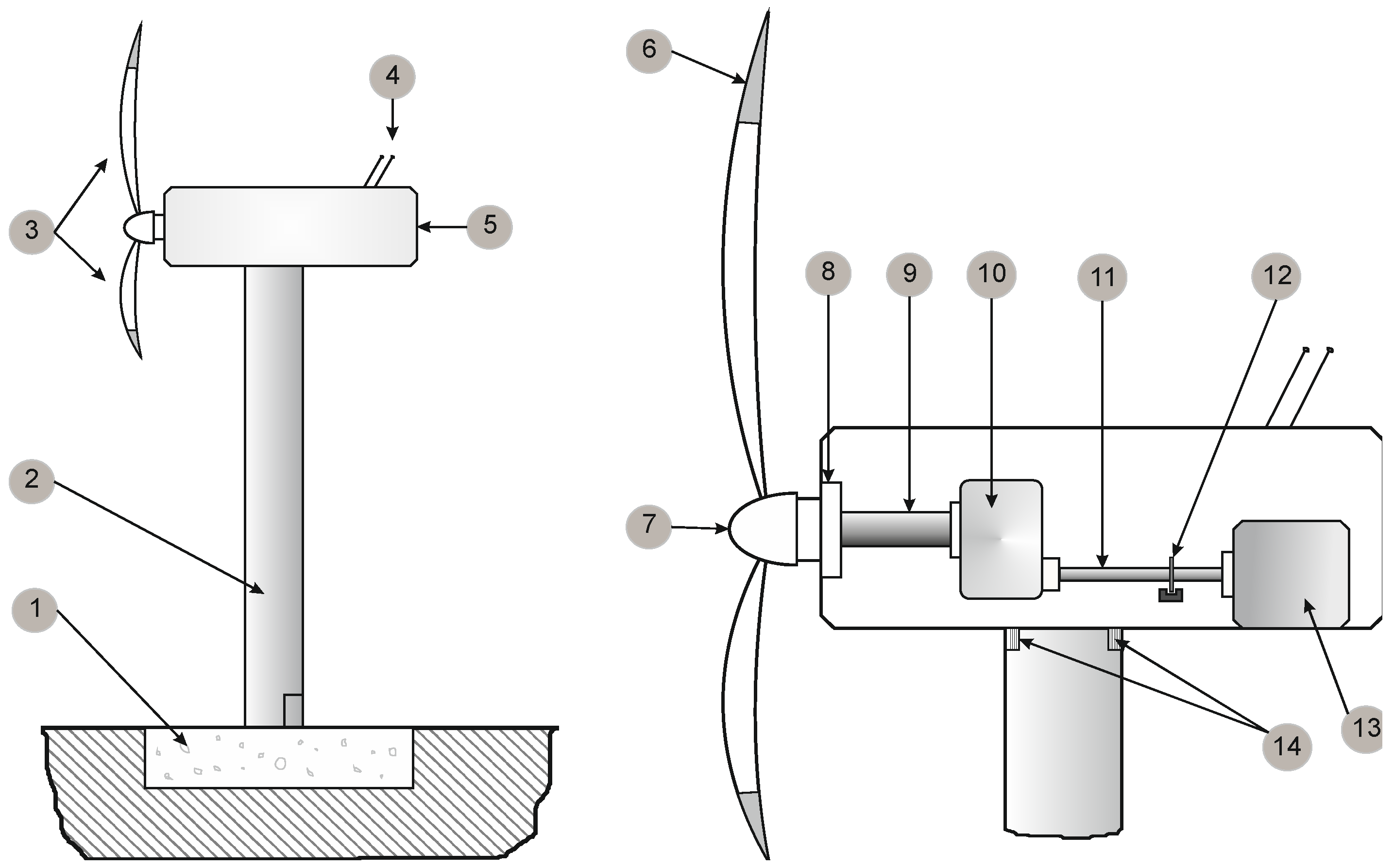
• A real case study is considered based on the research project OptiWindSeaPower.
• The DM in wind turbine manufacturing by a qualitative analysis that uses an LDT.
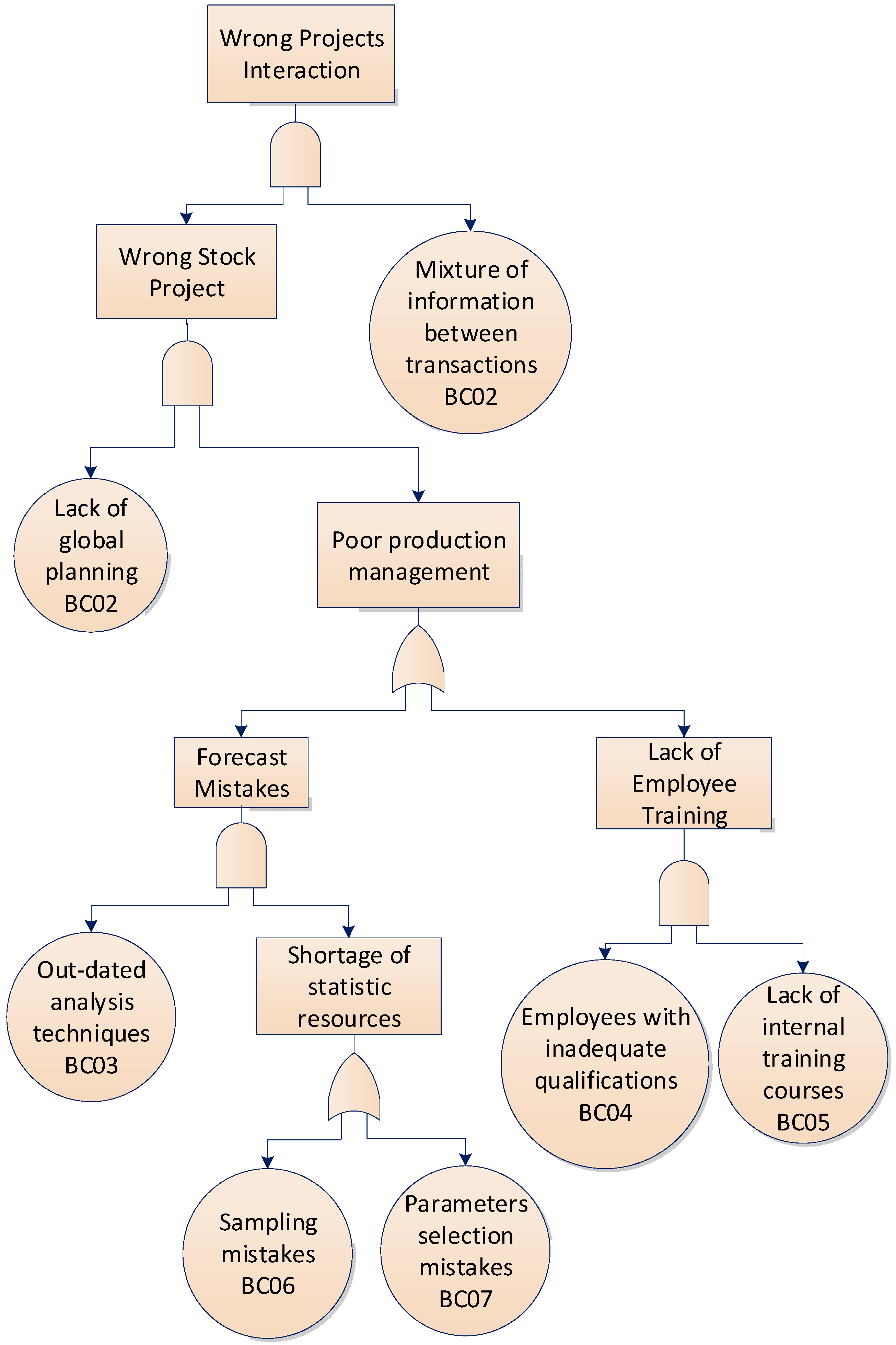
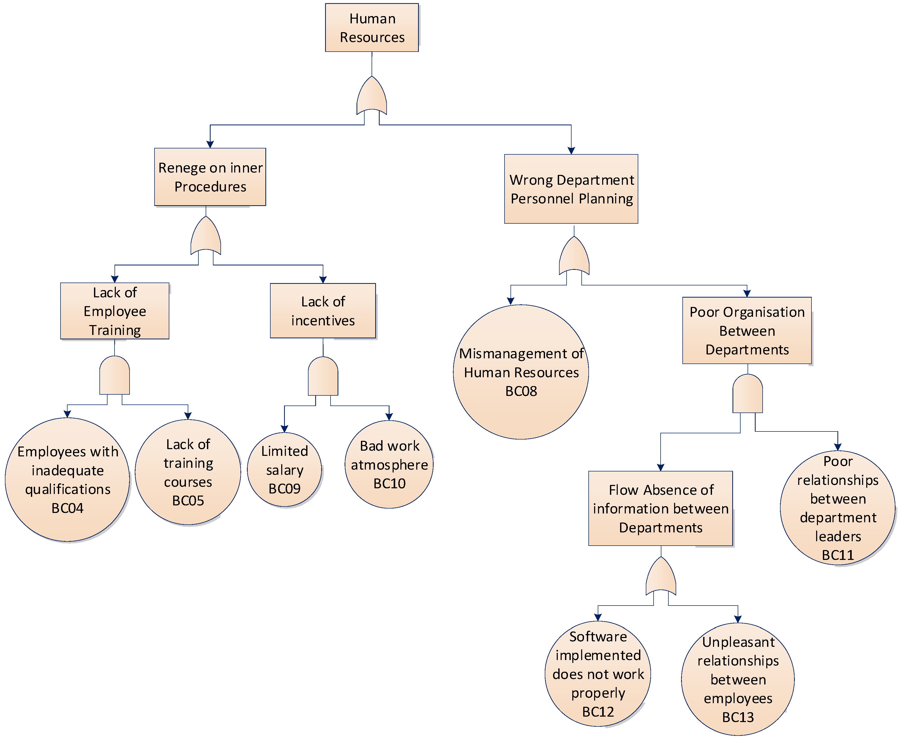
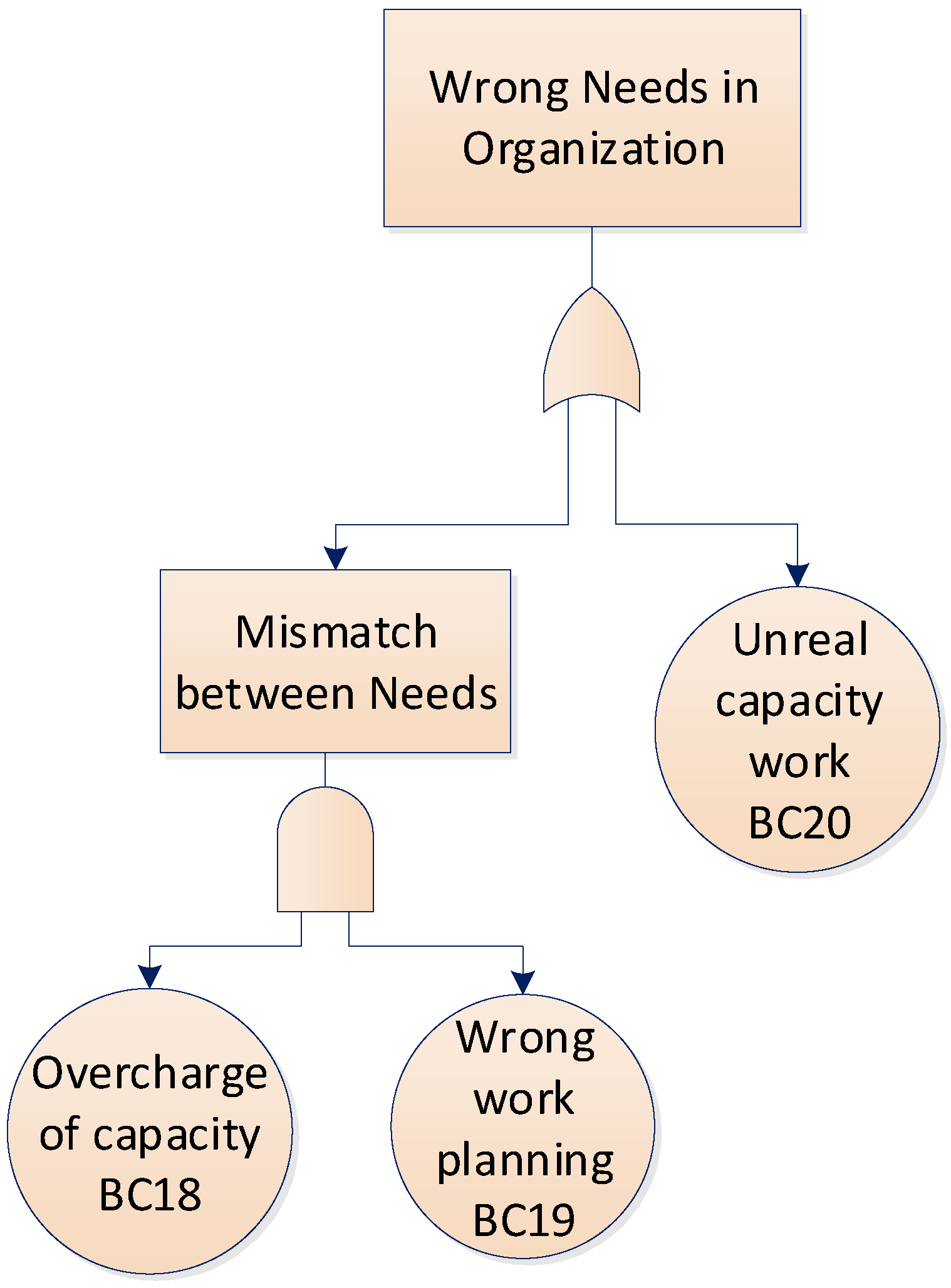
• A qualitative analysis of wind turbine manufacturing is proposed using logical decision trees.
• A quantitative analysis is carried out by using the BDD and analyzing the Boolean function.
• The optimization of the investments subject to the budget is employed based on importance measures.
• The problem is optimised over time.
• The computational cost is reduced by employing the ranking of the events methods of: Top-Down-Left-Right, Level, AND, Breadth-First Search (BFS) and Depth First Search (DFS) [20].
• Fussell-Vesely, Birnbaum, Criticality methods are employed to calculate the importance measures.

Section 2 discusses the LDT, BDD, the transformation from LDT to BDD and the importance measures [21]. A real case study based on the OptiWindSeaPower research project is described in Section 3. The results are shown and discussed in Section 4. Finally, Section 5 provides the main conclusions.

2. Logical Decision Tree and Binary Decision Diagrams

2.1. Logical Decision Trees

LDT analysis is given in Reference [22] considering the interrelation between every single basic cause (BC), i.e., events that cannot be broken down into other causes, and including the logical operators ‘AND’ and ‘OR’, that define the interrelations between causes [23,24]. The non-basic cause (NBC) is an event that can be broken down into other causes. An LDT considers a root cause, known as main problem (MP) or top event, and the relation between the MP and its causes [25].

Repeated BCs can be found because there are BCs that can be responsible for the MP in different business areas. BDDs are employed to analyze the LDT, shown in Figure 2.

2.2. Binary Decision Diagrams

BDD are employed to obtain the analytical expression of the MP occurrence probability, Q_MP. BDD is obtained from the LDT, enabling the Boolean function of Q_MP to be obtained. BDD is a directed graph, i.e., with no cycles, in which different events are interconnected by nodes that collect all the possible states. Each node or vertex is followed by two branches that determine the occurrence or non-occurrence of the corresponding event.

A data structure that represents the Boolean functions is the BDD [26]. They were extended by Akers [27] and Bryant [28,29] by the BDD canonical bases. BDD provides a new alternative to the traditional cut-set (CS) based approach for LDT that leads to the determination of the output value of the function through the examination of the values of the inputs [30].

A BDD is defined as a directed acyclic graph (V, N), V being the vertexes and N the indexes. There are two vertex types: A terminal vertex with value(v) of 0 or 1, where 1 corresponds to system failure, and 0 to system success. The CSs are given by the paths that have 1 state; the non-terminal vertex v has an index(v) ∈ N [0,1,…,n] and two descendants, high(v) and low(v) ∈ V, connected by a branch. The NBC is given by 0 branch, and the occurrence by 1. For any non-terminal vertex v, if high(v) is non-terminal, then index(v) < index(high(v)), else if low(v) is also non-terminal, then index(v) < index(low(v)). In other words, CSs are the paths “from the top to the ones” and each one of them provides a different scenario where the MP would occur.

When v is a non-terminal vertex with index(v) = 1, f_v given by Equation (1):

f_v(x₁,…,x_n) = x_i·_low(v)(x₁,…,x_n) + x_i·_high(v)(x₁,…,x_n).

(1)

If v is a terminal vertex with value(v) = 1, then f_v = 1, else if value(v) = 0 then f_v = 0.

The conversion from LDT to BDD is given by References [31] employing the following rules: changed-order; expansion; get-rid-of, and; absorption. Let V be a vertex set as V = V(v₁, …, v_n), if v₁, …, v_m are the v descendant vertices, then: index(V(v₁, …, v_n)) = min(index(G_i)), where 1≤ i ≤ n.

An example of the conversion from BDD to LDT is shown in Figure 2.

CSs are given by the paths that start from the first BC and finish in terminal vertices with 1 value from the BDD. The following CSs are given in Figure 2:

$$C{S}_1=B{C}_1·B{C}_3,$$

$$C{S}_2={BC}_1·\overline{B{C}_3}·{BC}_4,$$

$$C{S}_3=\overline{B{C}_1}·B{C}_2·B{C}_3,$$

$$C{S}_3=\overline{B{C}_1}·B{C}_2·\overline{B{C}_3}·B{C}_4.$$

P($B{C}_i$) is the occurrence probability of the i BC. Then, the MP occurrence probability, $Q_{MP}$, can be expressed as the sum the probabilities of all the CSs, since these CSs are mutually exclusive events. Therefore, $Q_{MP}$ is given by Equation (2):

$$Q_{MP}={{\displaystyle \sum }}_{i=1}^{N}P\left(C{S}_i\right),$$

(2)

where N is the total number of CSs, $P\left(C{S}_i\right)$ is the probability of occurrence of the i CS. This expression will represent the utility function in the DM process. $Q_{MP}$ is for the example:

$$\begin{array}{ll}{Q}_{MP}=& P(B{C}_1)·P\left(B{C}_3\right)+P(B{C}_1)·\left(1-P\left(B{C}_3\right)\right)·P\left(B{C}_4\right)+(1-P(B{C}_1))·P\left(B{C}_2\right)·P\left(B{C}_3\right)\\ & +(1-P(B{C}_1))·P\left(B{C}_2\right)·\left(1-P\left(B{C}_3\right)\right)·P\left(B{C}_4\right).\end{array}$$

The BDD size depends on the ordination of the BC [32]. The methods employed to obtain an index to BCs for ranking them close to the optimal are: Top-Down-Left-Right (TDLR) [33], the LDT is read from top to bottom and from left to right. The ranking is generated according to the order in which the BCs are found; the Malik et al. method [32] is based on the levels (Level). It is not a simple and direct method. It differentiates between the BCs depending on where they are located, i.e., it is directly related to the number of gates that are above them. The multiple occurring events are listed first when there are BCs in the same level; Xie et al. method [34], based on the AND gates (AND), establishes the importance of each BC_i by counting the number of AND gates on the path from the BC_i to the top event; Breadth-First Search (BFS) [35], the LDT is read from left to right and the BCs are ranked according to the order in which they are found; Depth First Search (DFS) [10], the LDT is read from top to bottom and in each level the left LDTs are read first. More details about the methods can be found in Reference [36].

A similar approach to analyze quantitatively the LDT via BDD was considered by Coudert and Madre [12] using MetaPrime. They demonstrate the BDD efficiency for small and large fault tree analysis from the computational cost point of view. In this paper, a set of smaller LDTs, similar to the size of the case study studied, have been employed to analyse the ranking methods.

Table 1. Logical decision trees (LDTs) characteristics.

LDT i	Basic Events	Intermediate Events	OR Gates	AND Gates	Levels
LDT 1	5	5	3	3	3
LDT 2	15	13	10	4	8
LDT 3	11	9	5	5	6
LDT 4	25	21	16	6	12
LDT 5	20	15	10	6	5
LDT 6	12	7	5	3	4
LDT 7	10	7	7	1	5
LDT 8	20	17	12	6	11
LDT 9	31	25	16	10	11

shows the number of basic events, intermediate events, OR and AND gates and levels for each LDT.

The number of CSs are given in

Table 2. Cut-sets (CSs) obtained by the ranking events.

LDT i	TDLR	DFS	BFS	Level	AND
LDT 1	2	2	2	2	2
LDT 2	30	30	155	30	30
LDT 3	12	24	36	12	12
LDT 4	64	142	176	64	22
LDT 5	99	207	257	99	55
LDT 6	9	7	7	9	9
LDT 7	9	12	21	9	9
LDT 8	44	76	192	44	44
LDT 9	1012	1292	3456	1012	1012

.

BFS provides poor results in most of the cases, especially when the LDT has a large number of events, levels and “OR” and “AND” gates. The Level and AND methods generate the ranking of the events with a minimal CSs. The conclusions regarding Level, DFS and TDLR methods should be studied for each LDT.

There is not a specific heuristic method for any LDT, i.e., the best method should be chosen for each LTD. The heuristic methods employed in this paper are static. There are also dynamic heuristic methods, however, they are not suitable for large or complex LDTs because they present some drawbacks, e.g., they need to store in memory the BDD or a part of it [37].

2.3. Importance Measures

Importance measures (IMs) are employed in this research in order to establish the most important BCs in a given time that affects the main cause that is being studied, i.e., they are employed for the LDT sensitivity analysis regarding the BCs [38]. The study will establish the BCs where it is necessary to focus on the investment of tasks. IM provides a weight index of the BC over the LDT [39,40].

The IMs can be classified into two main categories from the probabilistic perspective.

• Deterministic. They determine the importance of a BC without considering its occurrence probability.
• Probabilistic. They provide more details about the system than the deterministic IMs. The importance of the BC depends on its occurrence probability and its allocation into the LDT.

There are different methods to determine the IM, but they are not exact. This paper considers three methods in order to validate the results:

Fussell-Vesely Importance Measure $I^{FV}$ [41]. $I^{FV}$ is defined as the quotient between the CSs that contain a BC itself and Q_MP, given by Equation (3),

$$I_k^{FV}=\frac{P\left(C{S}_1{\displaystyle \cup }C{S}_2{\displaystyle \cup }\dots {\displaystyle \cup }C{S}_j\right)}{Q_{MP}},$$

(3)

where $I_k^{FV}$ is the $I^{FV}$ of the k BC, and $P\left(C{S}_1{\displaystyle \cup }C{S}_2{\displaystyle \cup }\dots {\displaystyle \cup }C{S}_j\right)$ is the probability of the union of the CSs that contains the k BC.

Birnbaum Importance Measure $I^{Birn}$ [42]. $I^{Birn}$ provides the value associated with the direct relation between Q_MP and the corresponding BC. It is defined by Equation (4),

$$I_k^{Birn}=\frac{\partial Q_{MP}}{\partial w_k},$$

(4)

where $I_k^{Birn}$ is the $I^{Birn}$ of the k BC, and $w_k$ is the probability assigned to the k BC.

Criticality Importance Measure $I^{Crit}$ [43]. $I^{Crit}$, unlike $I^{Birn}$, considers the probability of occurrence of the BC itself. It is given by Equation (5):

$$I_k^{Crit}=\frac{w_k}{Q_{MP}}·\frac{\partial Q_{MP}}{w_k}=\frac{w_k}{Q_{MP}}·I_k^{Birn},$$

(5)

where $I_k^{Crit}$ is $I^{Crit}$ of the k BC.

A detailed analysis of the methods employed is shown in Reference [18].

3. Real Case Study

A real case study based on the research project called OptiWindSeaPower is employed [44]. The case study considers a production delay given by the LDT, shown in Figure 3. 32 BCs and 23 intermediate causes are considered for wind turbine production delay, with 12 OR and 11 AND gates, shown in Figure 3, Figure 4, Figure 5, Figure 6, Figure 7 and Figure 8. The case study is simple, the main objective is to discuss the key features of the approach. It is discussed in more detail in Section 5.

Figure 4 shows the Wrong Projects Interaction LDT from Figure 3. It consists of 7 BCs and 5.

Figure 5 shows the Human Resources LDT, where the BC employees with inadequate qualifications and lack of internal training courses are the same BC, as shown in Figure 4. There are also 12 NBC and 8 BC, 4 OR and 3 AND gates.

Lack of Notification LDT is shown in Figure 6, with 7 BCs, where Out-dated analysis techniques; Sampling mistakes, parameters selection mistakes are also indicated in the LTD, as shown in Figure 5. It also considers 10 NBCs, the Forecast mistakes and Shortage of statistic resources as in Figure 4, with 3 OR and 3 AND gates.

Wrong needs in organization LTD, shown in Figure 7, is the simplest LTD. It shows 3 BCs and 1 NBC, with and 1 OR and 1 AND gates. It does not indicate any repeated BCs.

Finally, Figure 8 shows the Delay Orders LTD, with 7 BCs 4 NBC, and 2 AND and 2 OR gates.

Figure 9 shows the BCs probabilities of occurrence in time. The probabilities were set by experts in the research project [44]. They could change to other projects or over time. The objective is to calculate Q_MP is given by Equation (2), i.e., the occurrence probability of the Production Delay and then analyze the main causes for this scenario.

4. Results

The best method to reduce the size of the BDD, i.e., to minimize the number of CS, and, therefore, the computational cost, has been the AND-based criterion.

The order of the variables is:

$$\begin{array}{l}B{C}_{08}>B{C}_{20}>B{C}_{21}>B{C}_{26}>B{C}_{27}>B{C}_{04}>B{C}_{05}>B{C}_{01}>B{C}_{09}\\ \hspace{1em}\hspace{1em}>B{C}_{10}>B{C}_{11}>B{C}_{24}>B{C}_{25}>B{C}_{12}>B{C}_{13}>B{C}_{14}\\ \hspace{1em}\hspace{1em}>B{C}_{17}>B{C}_{18}>b_{19}>BC>B{C}_{23}>B{C}_{15}>B{C}_{16}>B{C}_{03}\\ \hspace{1em}\hspace{1em}>B{C}_{06}>B{C}_{07}>B{C}_{02}\end{array}$$

The CSs were 889, and the $Q_{MP}=83.04\%.$

The Fussell-Vesely, Birnbaum and Criticality IMs are presented in Figure 10 for the first month. They will be used to select the BC_i that will reduce their $P\left(C{S}_i\right)$, and, therefore, P(CS_i) where they appear and the Q_MP according to Equation (2).

Fussell-Vesely IM gives more importance to BC8, Mismanagement of Human Resources Department and BC4, employees with inadequate qualifications, and BC 5, Lack of Internal Training Courses. The results obtained by Birnbaum IM provide more balance between BCs, and they are similar to the Fussell-Vesely IM, but Birnbaum IM now gives more importance to BC16 and BC22 than BC14, and more importance to the BC26 and 27. Finally, Criticality IM provides similar results to Fussell-Vesely IM. Therefore, the results provided by the IM methods are similar for this month, where the results can then be validated.

The BC_i cost is shown in Figure 11. They were estimated in the research project [44] by the experts. This information, together with the previous results and those obtained by the IM, will provide the optimal DM for each BC_i.

The reduction of $Q_{MP}$, $Q_{MP}^{*}$, will be done by a reduction of the occurrence probability of BC_i, I(BC_i). The objective function is given by Equation (6),

$$minimize\hspace{1em}\hspace{1em}f\left(Q_{MP}^{*}\left(I\left(B{C}_i\right)\right)\right),$$

(6)

$$subject to\hspace{1em}\hspace{1em}{\displaystyle \sum }_{i=1}^n{C}_i·B{C}_i\le Budget$$

$$0\le I\left(B{C}_i\right)\le P_{B{C}_i},$$

where the objective function $f\left(Q_{MP}^{*}\left(I\left(B{C}_i\right)\right)\right)$ is a Non-Linear Programming Problem (NLPP), due to the Boolean function is given by Equation (2). The first constraint is defined by total investment is done in the BCs, ${{\displaystyle \sum }}_{i=1}^n{C}_i·B{C}_i$, where the investment in each BC_i, $C_i·B{C}_i$, is given by the BC_i cost, C_i, given in Figure 11, subject to the budget per month, in this case 400 €/month. When an investment is done to a BC_i, the probability of the BC_i will be I(BC_i), and, if there is no investment in the BC_i, then $I\left(B{C}_i\right)=w_{B{C}_i}$ and BC_i = 0, being $P_{B{C}_i}$ the probability assigned to each BC_i, given in Figure 9.

Figure 12 shows the investment distribution over time. The investments are done in the BC_i that have a major IM in each month subject to the budget.

The investment done in Figure 12 per month for each BC_i affects its occurrence probability I(BC_i). The new I(BC_i) per month are shown in Figure 13.

I(BC_i) over time, given in Figure 13, indicates that $Q_{MP}$ will be updated as $Q_{MP}^{*}\left(I\left(B{C}_i\right)\right)$ over time, shown in Figure 14. The reduction could be greater if the budget is larger. This is a case in which the firm could have a budget for 10 months, but the decision maker could consider a threshold for the reduction of the $Q_{MP}$ and, therefore, does not do any more investment when the threshold is reached, or the total budget is fixed, etc.

5. Discussion

A real case study of wind turbine manufacturing has been presented and analyzed. The problem is qualitatively studied using LDTs, that are set according to the research project [44]. The quantitative study is done considering the Boolean expression to set the Q_MP, that is obtained by the conversion of the LDT to the BDD. Q_MP, given by Equation (2), is the sum of the CS_s probabilities, that depends on the P(BC_i). The CSs in this case study were 889, and the $Q_{MP}=83.04\%$ according to the P(BC_i) given in Figure 9. The objective is to reduce $Q_{MP}$ by the investments in the BC_i that have more importance in time. The Fussell-Vesely, Birnbaum and Criticality methods are employed in this paper to calculate the IMs in order to validate their results. They are used to select the BC_i that will be reduced their $P\left(B{C}_i\right)$, and, therefore, the Q_MP is reduced. The new probability of the BC_i, $I\left(B{C}_i\right)$, requires an investment, $C_i·B{C}_i,$ due to the cost of the tasks, resources, etc. employed in this BC_i, given by $C_i$. All the investments done in time are subject to a budget, being 400 €/month in this case study.

The approach shows the investment optimization done in order to reduce the $Q_{MP}$ over time. The problem is an NP-hard problem. The complexity of the problem depends on the number of variables and the structure of the programming problem (objective function and constraints).

The Q_MP is reduced over time, see Figure 14. For example, if there is a total budget, the decision maker can set the month and the Q_MP to reach, etc.

Figure 10 shows the IMs in the first month. The IM methods show the same results, and it is the same over time. It has been employed to validate the results.

It is suggested that future research studies:

• Consider new larger and more complex case studies
• Employ new ranking methods that could improve the methods considered in this paper.
• Use new IM algorithms that can get better rankings of the BCs.
• Develop and apply new optimization methods to solve this problem, including mathematical optimization algorithms, e.g., Newton’s method and Gradient Descent, and direct search methods, e.g., Simplex method and the Nelder-Mead method, but the complexity of the problem may require the use of unconventional optimization algorithms, such as heuristics, e.g., Simulated Annealing, Deterministic Annealing, Tabu Search, Genetic Algorithms, Ant Systems, Neural Networks, etc.
• Consider new variables, e.g., exogenous variables, availability of resources, dynamic constraints, etc.
• Take into account the risk-based approach considering the probabilities and consequences.

6. Conclusions

The main problem in decision making for wind turbine manufacturing involves multiple cause occurrences. They can be broken down into basic causes where their interrelationships can be plotted using logical decision trees. Logical decision trees are employed to analyze the main problem qualitatively. They are converted to binary decision diagrams to get the Boolean equation to analyze the decision-making problem from a quantitative perspective. The computational cost to solve the problem depends on the binary diagram decision size, given by the ranking of the basic causes. The size is reduced by employing several heuristic methods for validating the ranking of the events: Top-Down-Left-Right, Level based method, AND based method, Breadth-First Search and Depth First Search. The AND based method generally provide better results in this case study.

Fussell-Vesely, Birnbaum and Criticality methods are employed to calculate the importance measures. The importance measures are employed to select the basic causes that require any task in order to reduce the main problem probability occurrence. The methods provide the same results in each iteration and, therefore, the results are validated. The occurrence probability of the basic event with more importance is reduced by carrying out investment in terms of the cost of the tasks, resources, etc. required, and all the investments done in time are subject to a budget. A static and dynamic study is presented in this paper to show the main results.

The basic causes occurrence probability of the logical decision tree studied in this paper are known. The new scenarios are calculated monthly, where the occurrence probability of the main problem is reduced over time considering the objective function, subject to the restrictions discussed.

References

1. Marugán, A.P.; Márquez, F.P.G.; Lev, B. Optimal decision-making via binary decision diagrams for investments under a risky environment. Int. J. Prod. Res. 2017, 55, 5271–5286. [Google Scholar] [CrossRef]
2. Marugán, A.P.; Márquez, F.P.G.; Pérez, J.M.P. Optimal maintenance management of offshore wind farms. Energies 2016, 9, 46. [Google Scholar] [CrossRef]
3. Vachon, W. Long-term o&m costs of wind turbines based on failure rates and repair costs. In Proceedings of the Proceedings WINDPOWER, American Wind Energy Association annual conference, Portland, OR, USA, 2–5 June 2002; pp. 2–5. [Google Scholar]
4. Pérez, J.M.P.; Márquez, F.P.G.; Hernández, D.R. Economic viability analysis for icing blades detection in wind turbines. J. Clean. Prod. 2016, 135, 1150–1160. [Google Scholar] [CrossRef]
5. Muñoz, C.Q.G.; Márquez, F.P.G.; Tomás, J.M.S. Ice detection using thermal infrared radiometry on wind turbine blades. Measurement 2016, 93, 157–163. [Google Scholar] [CrossRef]
6. Muñoz, C.Q.G.; Márquez, F.P.G. A new fault location approach for acoustic emission techniques in wind turbines. Energies 2016, 9, 40. [Google Scholar] [CrossRef]
7. Pérez, J.M.P.; Márquez, F.P.G.; Tobias, A.; Papaelias, M. Wind turbine reliability analysis. Renew. Sustain. Energy Rev. 2013, 23, 463–472. [Google Scholar] [CrossRef]
8. Han, D.; Heo, Y.; Choi, N.; Nam, S.; Choi, K.; Kim, K. Design, fabrication, and performance test of a 100-w helical-blade vertical-axis wind turbine at low tip-speed ratio. Energies 2018, 11, 1517. [Google Scholar] [CrossRef]
9. de da González-Carrato, R.R.; Márquez, G.; Pedro, F.; Papaelias, M. Vibration-based tools for the optimisation of large-scale industrial wind turbine devices. Int. J. Cond. Monit. 2016, 6, 33–37. [Google Scholar] [CrossRef]
10. Cormen, T.H.; Leiserson, C.E.; Rivest, R.L.; Stein, C. Introduction to Algorithms; Mit Press: Cambridge, MA, USA, 1990. [Google Scholar]
11. Dale, M.; Krumdieck, S.; Bodger, P. A dynamic function for energy return on investment. Sustainability 2011, 3, 1972–1985. [Google Scholar] [CrossRef]
12. Coudert, O.; Madre, J.C. Towards an interactive fault tree analyser. In Proceedings of the IASTED International Conference on Reliability, Quality Control and Risk Assessment, Washington, DC, USA, 4–6 November 1992. [Google Scholar]
13. Fülöp, J. Introduction to Decision Making Methods; BDEI-3 workshop; Citeseer: Washington, DC, USA, 2005; pp. 1–15. [Google Scholar]
14. Wan, S.-P.; Wang, F.; Dong, J.-Y. A novel group decision making method with intuitionistic fuzzy preference relations for rfid technology selection. Appl. Soft Comput. 2016, 38, 405–422. [Google Scholar] [CrossRef]
15. Cascetta, E.; Carteni, A.; Pagliara, F.; Montanino, M. A new look at planning and designing transportation systems: A decision-making model based on cognitive rationality, stakeholder engagement and quantitative methods. Transp. Policy 2015, 38, 27–39. [Google Scholar] [CrossRef]
16. Xu, Y.; Patnayakuni, R.; Wang, H. Logarithmic least squares method to priority for group decision making with incomplete fuzzy preference relations. Appl. Math. Model. 2013, 37, 2139–2152. [Google Scholar] [CrossRef]
17. Manupati, V.; Anand, R.; Thakkar, J.; Benyoucef, L.; Garsia, F.P.; Tiwari, M. Adaptive production control system for a flexible manufacturing cell using support vector machine-based approach. Int. J. Adv. Manuf. Technol. 2013, 67, 969–981. [Google Scholar] [CrossRef]
18. Wu, D.D.; Chen, S.-H.; Olson, D.L. Business intelligence in risk management: Some recent progresses. Inf. Sci. 2014, 256, 1–7. [Google Scholar] [CrossRef]
19. Márquez, F.P.G. A new method for maintenance management employing principal component analysis. Struct. Durab. Health Monit. 2010, 6, 89–99. [Google Scholar]
20. Wu, D.D.; Olson, D.L.; Luo, C. A decision support approach for accounts receivable risk management. IEEE Trans. Syst. Man Cybern. Syst. 2014, 44, 1624–1632. [Google Scholar] [CrossRef]
21. Marugan, A.P.; Marquez, F.P.G. Decision-Making Management: A Tutorial and Applications; Academic Press: San Diego, CA, USA, 2017. [Google Scholar]
22. Dixit, V.; Srivastava, K.R.; Chaudhuri, A. Project network-oriented materials management policy for complex projects: A fuzzy set theoretic approach. Int. J. Prod. Res. 2015, 53, 2904–2920. [Google Scholar] [CrossRef]
23. Garc, F.P.; Pliego, A.; Trapero, J.R. A new ranking method approach for decision making in maintenance management. In Proceedings of the Seventh International Conference on Management Science and Engineering Management; Springer: Berlin/Heidelberg, Germany, 2014; pp. 27–38. [Google Scholar]
24. Huvenne, V.A.I.; Robert, K.; Marsh, L.; Iacono, C.L.; Bas, T.L.; Wynn, R.B. Rovs and auvs. In Submarine Geomorphology; Springer: Cham, Switzerland, 2018; pp. 93–108. [Google Scholar]
25. Lopez, D.A.; Van Slyke, W.J. Logic tree analysis for decision making. Omega 1977, 5, 614–617. [Google Scholar] [CrossRef]
26. Marugán, A.P.; In, F. Fault-tree dynamic analysis. In Proceedings of the Eleventh International Conference on Condition Monitoring and Machinery Failure Prevention Technologies CM, Manchester, UK, 10–12 June 2014; pp. 1–9. [Google Scholar]
27. Marugán, A.P.; Márquez, F.P.G.; Lavirgen, J.L. Decision making via binary decision diagrams: A real case study. In Proceedings of the Eighth International Conference on Management Science and Engineering Management; Springer: Berlin/Heidelberg, Germany, 2014; pp. 215–222. [Google Scholar]
28. Marugán, A.P.; Márquez, F.P.G.; Papaelias, M. Multivariable analysis for advanced analytics of wind turbine management. In Proceedings of the Tenth International Conference on Management Science and Engineering Management; Springer: Singapore, 2017; pp. 319–328. [Google Scholar]
29. Lee, C.-Y. Representation of switching circuits by binary-decision programs. Bell Labs Tech. J. 1959, 38, 985–999. [Google Scholar] [CrossRef]
30. Akers, S.B. Binary decision diagrams. IEEE Trans. Comput. 1978, 27, 509–516. [Google Scholar] [CrossRef]
31. Bryant, R.E. Graph-Based Algorithms for Boolean Function Manipulation; Carnegie Mellon University School of Computer Science: Pittsburgh, PA, USA, 2001. [Google Scholar]
32. Bryant, R.E. Binary decision diagrams. In Handbook of Model Checking; Springer: Cham, Switzerland, 2018; pp. 191–217. [Google Scholar]
33. Pliego, A.; Márquez, F.P.G. Big data and web intelligence: Improving the efficiency on decision making process via bdd. In Handbook of Research on Trends and Future Directions in Big Data and Web Intelligence; IGI Global: Hershey, PA, USA, 2015; pp. 190–207. [Google Scholar]
34. Márquez, F.P.G.; Marugán, A.P.; Papaelias, M. Introductory chapter: An overview to the analytic principles with business practice in decision making. In Decision Making; IntechOpen: Rijeka, Croatia, 2018. [Google Scholar]
35. Malik, S.; Wang, A.R.; Brayton, R.K.; Sangiovanni-Vincentelli, A. Logic verification using binary decision diagrams in a logic synthesis environment. In Proceedings of the 1988 IEEE International Conference on Computer-Aided Design ICCAD-88 Digest of Technical Papers, Santa Clara, CA, USA, 7–10 November 1988; pp. 6–9. [Google Scholar]
36. Bartlett, L.M. Progression of the binary decision diagram conversion methods. In Proceedings of the 21st International Systems Safety Conference, Ottawa, Canada, 2–4 August 2003. [Google Scholar]
37. Xie, M.; Tan, K.; Goh, K.; Huang, X. Optimum prioritisation and resource allocation based on fault tree analysis. Int. J. Qual. Reliab. Manag. 2000, 17, 189–199. [Google Scholar] [CrossRef]
38. Jensen, R.M.; Veloso, M.M. OBDD-based universal planning for synchronized agents in non-deterministic domains rune m. J. Artif. Intell. Res. 2000, 13, 189–226. [Google Scholar] [CrossRef]
39. Márquez, F.G.; Marugán, A.P.; Pérez, J.P.; Hillmansen, S.; Papaelias, M. Optimal dynamic analysis of electrical/electronic components in wind turbines. Energies 2017, 10, 1111. [Google Scholar] [CrossRef]
40. Nikolskaïa, M.; Rauzy, A.; Sherman, D.J. Almana: A BDD minimization tool integrating heuristic and rewritingmethods. In Formal Methods in Computer-Aided Design; Springer: Berlin/Heidelberg, Germany, 1998; pp. 100–114. [Google Scholar]
41. Marugán, A.P.; Márquez, F.P.G.; Lorente, J. Decision making process via binary decision diagram. Int. J. Manag. Sci. Eng. Manag. 2015, 10, 3–8. [Google Scholar]
42. Marugán, A.P.; Márquez, F.P.G. Improving the efficiency on decision making process via BDD. In Proceedings of the Ninth International Conference on Management Science and Engineering Management; Springer: Berlin/Heidelberg, Germany, 2015; pp. 1395–1405. [Google Scholar]
43. Márquez, F.; Pliego, A.; Ruiz, R. Fault detection and diagnosis, and optimal maintenance planning vía ft and BDD. In Proceedings of the Twelfth International Conference on Condition Monitoring and Machinery Failure Prevention Technologies from Sensors through Diagnostics and Prognostics to Maintenance CM, Oxford, UK, 9–11 June 2015. [Google Scholar]
44. Fussell, J. How to hand-calculate system reliability and safety characteristics. IEEE Trans. Reliab. 1975, 24, 169–174. [Google Scholar] [CrossRef]
Figure 1. Components of the WT: 1-Foundation; 2-Tower; 3-Blades; 4-meteorological unit; 5-Nacelle; 6-Pitch system; 7-Rotor hub; 8-Main bearing; 9-High speed shaft; 10-Gearbox; 11-Low speed shaft; 12-Brake system; 13-Generator; 14-Yaw system [7].
Energies 12 01753 g001
Figure 2. Example of Conversion from LDT to binary decision diagrams (BDD).
Energies 12 01753 g002
Figure 3. Wind turbine production delay LDT.
Energies 12 01753 g003
Figure 4. Wrong projects interaction LDT.
Energies 12 01753 g004
Figure 5. Human resources LDT.
Energies 12 01753 g005
Figure 6. Lack of notification LDT.
Energies 12 01753 g006
Figure 7. Wrong detailed needs in the organization LTD.
Energies 12 01753 g007
Figure 8. Delay orders LTD.
Energies 12 01753 g008
Figure 9. Basic causes (BCs) probabilities of occurrence.
Energies 12 01753 g009
Figure 10. Fussell-Vesely, birnbaum and criticality importance measures (IMs).
Energies 12 01753 g010
Figure 11. Cost of BCi.
Energies 12 01753 g011
Figure 12. Investments per month and per BCi with a budget of 400 € per month.
Energies 12 01753 g012
Figure 13. Occurrence probability reduction of each BCi over time.
Energies 12 01753 g013
Figure 14. Q M P over time.
Energies 12 01753 g014