A Methodology for Measuring the Heat Release Efficiency in Bubbling Fluidised Bed Combustors


Chair of Energy Process Engineering, Friedrich-Alexander-University, Erlangen-Nürnberg, Fürther Str. 244f, 90429 Nuremberg, Germany
*
Author to whom correspondence should be addressed.
Energies 2020, 13(10), 2420; https://doi.org/10.3390/en13102420
Submission received: 18 March 2020
/
Revised: 30 April 2020
/
Accepted: 30 April 2020
/
Published: 12 May 2020
(This article belongs to the Collection Bioenergy and Biofuel)
Abstract
:Differences in the densities of bed material and—especially biogenic—solid fuels prevent an ideal mixture within bubbling fluidised bed (BFB) combustors. So, the presence of fuel particles is usually observed mainly near the surface of the fluidised bed. During their thermal conversion, this leads to a release of unburnt pyrolysis products to the freeboard of the combustion chamber. Within the further oxidation, these species will not transfer their heat-of-reaction to the inert bed material in the way of a convective heat transfer, but rather increase the gas phase temperature providing probably some additional radiative heat transfer to the dense bed. In this case, the so-called heat release efficiency to the fluidised bed, being the ratio of transferred heat to the fuel input, will be reduced. This paper presents a methodology to quantify this heat release efficiency with lab-scale experiments and the observed effects of common operating parameters like bed temperature, fluidisation ratio and fuel-to-air ratio. Experimental results show that the air-to-fuel ratio dominates the heat release efficiency, while bed temperature and fluidisation ratio have minor influences.
1. Introduction
The principle of fluidised beds for thermal conversion of solid fuels is well-known since Winkler’s patent in 1923 with its focus on coal gasification. In the 1970s, the efforts for the development of bubbling fluidised bed (BFB) coal combustion raised rapidly [1]. First, power-plants like in Rivesville (USA) were still based on a bubbling fluidised bed combustion principle [2]. Some years later, the circulating fluidised bed (CFB) combustion aiming at higher power capacities started to succeed in research and industry [3]. With the rise of renewable energy sources, fluidised bed combustion was found to be highly interesting also for the thermal conversion of biomass. The key challenges for the combustion of biomass are ash-related aspects resulting from their higher inorganic content and especially their lower ash-melting temperatures, which cause severe slagging phenomena in grate furnaces [1,4,5,6,7,8]. Fluidised bed combustion, in contrast, offers an isothermal temperature distribution within the bed to face these problems, but also with a beneficial emission behaviour concerning nitrogen-oxides and the possibility of an in-situ desulphurisation [3,6]. Ash-related issues also occur for fluidised beds in this case, however, by showing a tendency for bed material agglomeration [9,10]. Moreover, compared to coal or lignite, solid biofuels typically have lower densities, which also highly affects the combustion characteristics in a fluidised bed. Due to the hydrostatic principle, fuel particles can accumulate in the upper part of the fluidised bed in a bubbling fluidised bed combustion setup. Especially during their devolatilisation, this will lead to a gas release directly in the freeboard region, with a combustion or rather heat production above the surface of the fluidised bed. For concepts with in-bed heat exchangers (e.g., with a Stirling engine in small-scale combined heat and power applications [11]) this will directly influence the maximum transferable heat. In such a case, an operation at a maximised heat output will be key for the achievement of the highest possible electrical efficiency. In order to quantify these combustion conditions, we define a heat release efficiency , which is the ratio of the in-bed released heat of combustion to the fuel energy input :
2. Mixing of Fuel Particles in Bubbling Fluidised Beds
To the present, it is hard to state a common consensus regarding the mixing and segregation effects of fuel and bed material in fluidised beds, which would allow a spatially resolved description for the time-depending positions of fuel particles depending on the fluidisation conditions. Rowe et al. [12] describe cold-flow experiments in order to find correlations for a segregation depending on densities, particle diameters and fluidisation velocities. They report that the mixing depends highly on the fluidisation velocity U and that high fluidisation ratios (with being the minimum fluidisation velocity) are required to achieve a nearly complete mixing. These results correlate with similar data from [13], who observed that an ideal mixing will occur only at significantly increased fluidisation velocities. Santos and Goldstein [14] also performed measurements on a cold flow fluidised bed. They report that the quality of the mixing can be improved at higher fluidisation ratios, fuel density and particle diameter and postulate that this would have a notable effect on the pyrolysis, namely a release of products into the fluidised bed region. In a more detailed way, this is described in the work of Gómez-Barea et al. [15], who identified several segregation effects depending on the particle properties. Especially for the fluidised bed gasification they expect increased amounts of tar contents in the produced syngas as a consequence of this non-ideal mixing.
Compared to these investigations with an evaluation of images taken from more or less two-dimensional fluidised beds, several authors developed improved methodologies for experiments with an extended width of fluidised beds. Wirsum [16] used a setup with magnetic particles in a fluidised bed. He was able to detect the three-dimensional positions by using several coils at different locations and identified the same influences on the mixing behaviour. Another simple method for the location of fuel-like particles is the so-called freezing. In such experiments, the air supply for a fluidised bed is stopped at steady-state conditions, so that the bed collapses immediately. By removing several layers of bed material and counting the fuel-like particles, an axial concentration of the fuel distribution can be reconstructed. Zhang [17] applied this methodology in his studies, observing a high segregation of biomass particles for an operation slightly above the minimum fluidisation velocity. An increase of air mass flow supports the mixing, although the fuel particles were still located largely in the upper third of the bed. However, for fluidisation ratios , he again reports a segregation process. In this case, bubbles transport the biomass particles to the freeboard region, influencing the previously observed mixing within the fluidised bed. Optical measurements in [18] confirmed this observation.
Experiments with reacting particles were conducted by Bruni et al. [19]. They optically detected particles during their pyrolysis and describe the fact that released volatiles form additional gas layers around the particles. This enhances the particle transport to the surface by creating an additional uplift. However, it must be mentioned that the fluidised bed was operated with low gas velocities slightly above the minimum fluidisation. This obviously causes the segregation of bed material and fuel particles. In 2007, Cui [20] reviewed present work related to the mixing behaviour in fluidised bed. He stated that, so far, still little knowledge is available for inert particles, let alone for reacting particles, for example, during the pyrolysis. Li et al. reported the visualisation of single reacting lignite particles in a two-dimensional pressurised oxy-fuel combustion with a pre-calibrated two-colour pyrometry. They had a special focus on the investigation of ignition, volatiles and char combustion at different atmospheres [21].
There is also some recently published work from the Chalmers University related to this work. Sette et al. presented a camera-probe based fuel tracking system [22]. With this system, they are able to investigate the distribution of fuel particles at the surface of their bubbling fluidised bed at hot conditions of 800 °C in gasification mode. They clearly identified an improved mixing with an increasing excess velocity. Köhler et al. [23] presented and validated a mathematical approach to describe the mixing in the fluidised bed. This model predicts an increased residence probability near the surface of a fluidised bed for decreasing fuel densities. They also state that—independent from density or particle size—increased fluidisation ratios always support the vertical mixing.
In 2002, Scala et al. [24] suggested a one-dimensional model for predicting the heat release efficiency in fluidised bed combustion. They divide the fluidised bed in three regions, the dense bed itself, a transition region with the splash-zone and the freeboard. The regions are coupled with a description of the bed’s hydrodynamic behaviour as well as with energy equations. They particularly focused on the modelling of the splash-zone, as a significantly high amount of heat will be transferred by convection and radiation mechanisms back to the surface of the bed. They described that the calculated heat release efficiency of their model highly depends on the fluidisation ratio, although they presented data only for so far. Two years later Scala applied this model for several solid fuels at and a fluidised bed consisting of bed particles with a diameter of mm at a temperature of 850 °C. For these conditions, the model provides a fuel-depending heat release efficiency in the range of 75% to 99% [25].
As described, it is especially hard to describe the mixing of reacting particles within a fluidised bed at high temperatures and to have a forecast of their positions along their thermal conversion. As there is no available model of the downstream mixing between gaseous products of the fuel and the oxidation agent linked to the solid mixing, we are not able to describe or to calculate time and place of the combustion process. Especially, a detailed modelling of the overlapping combustion within the dense bed, the splashing-zone and the freeboard requires experimental data, for example, with the presented method to investigate the heat release.
3. Methodology
This paper introduces an experimental methodology for determining the heat release efficiency at a laboratory scale fluidised bed combustion plant. Actually, the basic idea was already presented in 2007 by Ottmann [26]. However, due to his neglection of the spatial resolution of the combustion process, this paper suggests some modifications of Ottman’s method, as described later on.
3.1. Mathematical Description
In principle, the model starts with an energy balance of the fluidised bed, as shown in Figure 1.
It contains the incoming mass flow of combustion air with its temperature and specific heat capacity , respectively, a flue gas mass flow . Enthalpy, more specifically, specific heat capacity refers to 0 °C as we use no absolute temperatures. In order to describe an only partial heat release within the fluidised bed, the thermal capacity is multiplied with an appropriate heat release efficiency (see Equation (1)). Due to fuel temperatures being typically in the range of ambient temperatures, the input of the fuel’s sensible heat is neglected, while heat losses of a fluidised bed combustion chamber have to be taken into account.
In a steady-state operation, the sum of incoming and outgoing heat fluxes have to be equal:
Replacing the overall heat fluxes with products of mass flows, temperatures and specific heat capacities, or in the case of the fuel input , the mass flow multiplied by the heating value , provides the following expression:
For such operating conditions, a determination of is hardly possible, as the losses are more or less unknown. Furthermore, it would require an adequate period of operation at constant bed temperature.
However, an increasing bed temperature due to the combustion in a non-steady case can be considered by inserting an additional term of a heat sink in the previously mentioned energy balance (Equation (4)). Assuming a nearly constant heating rate , it has to be multiplied with the heat capacity of the fluidised bed reactor , which represents mainly bed material and steelwork:
After stopping the fuel supply, the fluidised bed will cool down in accordance to
with an appropriate cooling rate . As there is no fuel mass flow, the mass flows of in- and outgoing air are constant.
Subtraction of Equations (5) and (6)
eliminates the unknown heat losses as well as the input of sensible heat by the combustion air.
With the assumption that each outflow temperature matches the fluidised bed temperature (), Equation (7) provides the expression
for the heat release efficiency . Now most of the remaining parameters are more or less accessible during the operation of a lab-scale fluidised bed combustion plant.
For an estimation of the heat capacity , the sum of each heat capacity (bed material and steel) by multiplying mass and specific heat capacity is sufficient for a first estimation. A more proper way of determining within the experiment is possible in several ways, each with a defined heat input like an electrical bed heater or an equivalent heat sink (e.g., in-bed heat exchangers). In this case, was determined with the electrical bed heater of the fluidised bed combustor, as described later on. For this electrical heat-up curve without any fuel input, but a given input of the electrical bed heater , a modified energy balance
is valid. Together with Equation (6) for the cool-down process, the relation between and is given by:
Another challenge is the estimation of an appropriate value for the specific heat capacity of the flue gas . Assuming a fairly entire reaction in a chemical equilibrium, the flue gas composition and as a result the specific heat capacity can be easily calculated. For an only partial oxidation reaction within a fluidised bed, flammable gases (e.g., CO, CH4…) and volatiles with significantly higher specific heat capacities will remain in this product gas. This would require an adequate modelling approach. However, the choice of conditions corresponding to a chemical equilibrium with an error estimation provides already feasible results.
In comparison to our approach, Ottmann made some simplifications. First of all, he neglected the difference between the heat capacities of flue gas and air , as well as the additional mass flow due to the fuel input (). Otherwise, he stated that only a short duration of fuel input (e.g., 2 min) of a defined fuel mass will result in a constant temperature shift of the fluidised bed compared to a cooling-down curve. With these assumptions, he gets a simplified equation for an evaluation of [26]:
However, first experimental tests according to this methodology showed some weaknesses: Within this short period of fuel feeding, we will not reach steady-state conditions of the gas composition in the fluidised bed. When starting the fuel input, the drying and pyrolysis mechanism will be the first step of fuel conversion. For wood pellets in a fluidised bed of 800 °C, this process will take approximately one minute [27]. The char conversion starts mainly after a nearly complete release of the volatiles and will last much longer than pyrolysis [28]. So for a fuel feeding of only several minutes, it is obvious that these conditions will not correspond to conditions of a continuously operating fluidised bed combustion. Ottman’s methodology represents combustion at unrealistic high excess air in case of only little fuel input, or varying fuel-to-air ratios for an increased mass of fuel. In order to identify the presence of constant conditions, at which a reliable evaluation of the heat release efficiency is possible, the value of the air-to-fuel ratio is appropriate. First tests showed, that this requires a duration of about 10 to 15 min until steady state-conditions can be ensured. In the end after stopping the fuel input, it also lasts several minutes for the conversion of the resulting char, also coming along with a slight increase of the air-to-fuel ratio. For a better illustration, this time-dependent behaviour is shown in Figure 2 with a schematic plot of the air-to-fuel ratio.
3.2. Experimental Implementation
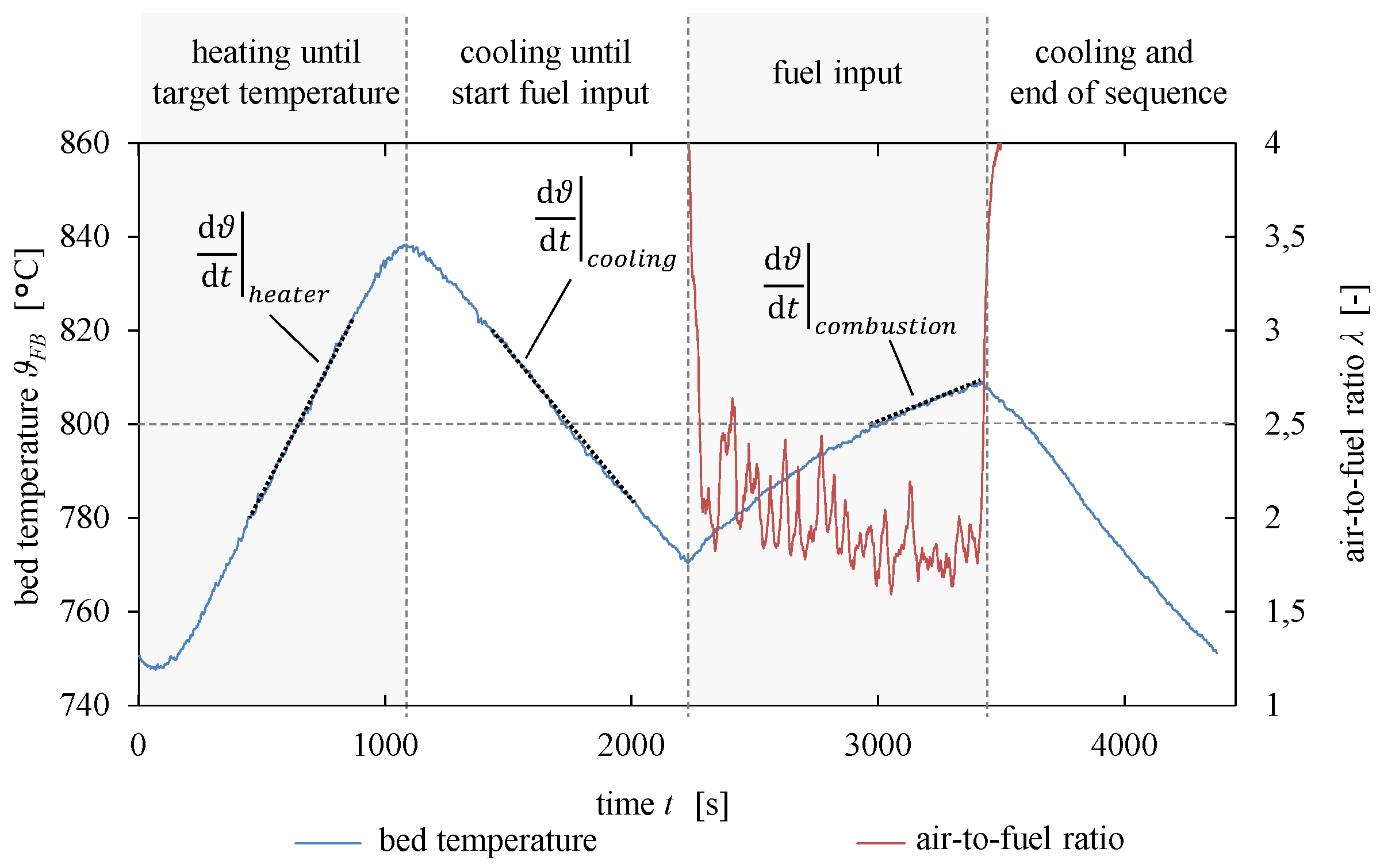
An experimental investigation of the heat release efficiency according to Equation (8) for a given temperature requires primarily a heating-up curve during combustion of a particular fuel and a cooling-down curve without fuel input while all other conditions of the fluidised bed reactor are kept constant (see Figure 3 for a target bed temperature of 800 °C). Additionally, for the already mentioned method, this procedure has to be extended by recording an electrical heating-up curve. In order to realise a time efficient sequence, it starts in a reverse order.
A key challenge for this method is to gain constant temperature gradients in the range of the desired target temperature. For this purpose, in each case a superheating or rather supercooling of 30 to 80 K was provided. In the end, an analysis of these three temperature means the evaluation of linear regression curves in these ranges.
4. Experimental Setup
For this study, a bubbling fluidised bed combustion plant at the Institute of Energy Process Engineering was used with different fuels.
4.1. Plant Setup
The test facility with a maximum thermal input of 100 was developed and installed in the year 2012 with respect to fuel and bed material tests, validation tasks of CFD-models, but also a coupling with thermal engines like a Stirling Engine in the sense of a combined heat and power plant [11] was considered during construction.
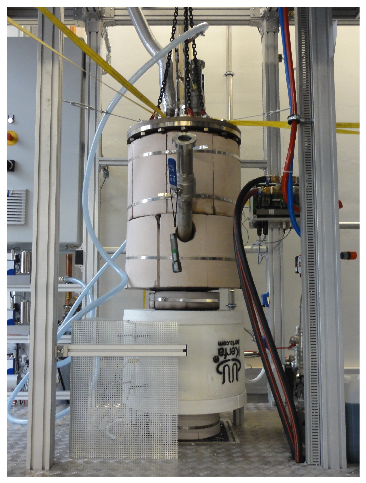
Because of this reason, the plant features a simple and modular assembly of several parts made from the high temperature steel 1.4841 with each segment having a height of 400 . The fluidised bed area itself has a diameter of 200 and a height of 400 , and in the freeboard region, a conical shape extends the diameter to 400 . The fuel feeding is realised by means of a screw feeder through a downpipe to the bed surface. Combustion air enters the fluidised bed through a porous plate at the bottom and can optionally be pre-heated up to 400 °C. An electrical bed heater with a load of 9 supports the start-up process and the determination of the plants’ heat capacity. Together with an appropriate high temperature insulation, the start-up process takes about one and a half hours for reaching the ignition temperature of typical solid fuels like wood pellets or about two hours to achieve bed temperatures in the range of 800 °C. Figure 4 shows the assembled plant in its configuration for the presented experiments with an overall height of 1600 . Additional secondary air is injected through a pipe from the cover flange into the conical section of the freeboard. A PLC system of Bernecker and Rainer is responsible for controlling the whole plant operation and the required data logging. The programming of the time-depending sequence of the presented methodology in Figure 3 allows to carry out parameter variations in an automated manner.
The combustion itself is controlled by adjusting the corresponding mass-flows of fuel and air. As we like to keep constant fluidisation numbers, the air mass-flow controlled by a mass-flow-controller is fixed for each ratio of . The known fuel composition allows a calculation of the stoichiometric air demand. Considering the desired air-to-fuel ratio , it is possible to adjust the fuel mass flow with a calibrated fuel feeding screw. Finally, a lambda sensor serves only for the measurement and monitoring of the air-to-fuel ratio.
Although there is an implemented PID controller for the bed heater to achieve constant bed temperatures, for this methodology it is only necessary to operate the heater at defined electrical power consumption as we do not have to achieve steady-state conditions. Hence, the measurement of the current and the voltage of the resistance heater provides the information for our evaluation.
Common silica sand with a nominal diameter range of 0.1 to 0.6 mm (measured Sauter diameter approximately , at 800 °C) serves as bed material, as this particle size distribution allows a wide variation of the fluidisation number in the presented experimental setup. Depending on the thermal management of the 100 fluidised bed combustion plant, it can operate in the range of without a significant loss of bed material to the flue gas duct. However, for coarser bed materials, the capacity of the electrical bed heater would not be sufficient to measure the electrical heat-up curves, whereas a lower bed material diameter with a lower demand of fluidisation gas would cause a reduction of the fuel input to just a few kilowatts. In this case, the effect of a discontinuous fuel feeding with strong fluctuations of the fuel-to-air ratio would become predominant.
For determining the influence of the fuel-to-air ratio , operating conditions of the fluidised bed were in the range . For each experiment with , an additional secondary air mass flow needs to be chosen in order to ensure a complete oxidation of flammable components at a global of 1.5. This will also lead to the effect that radiative heat transfer from the freeboard area to the bed surface as an integral mechanism will be included.
4.2. Fuel Variation
During the experiments, three different types of solid fuels were used. Wood pellets represent a standardized biofuel with about 80% of volatile matter, while crushed lignite on the other hand is characterised by a higher amount of fixed carbon. In addition, lenticular polyethylene granules are supposed to pyrolyse within a few seconds entirely to volatiles without remaining char or ash components [29,30]. The respective fuel parameters are summarised in Table 1.
Concerning the fluidisation behaviour of the fuel, it is hard so state some fluidisation properties. As the particle size is one magnitude larger than the bed material and the densities being in the range of the fluidised bed itself, we can assume a minimum fluidisation according to Ergun’s equation being also multiple times higher than of the used silica sand. However, since the mass fraction of fuel in the bed of a bubbling fluidised combustion chamber is quite low compared to the bed material, we expect no significant effect on the fluidisation behaviour of the mixture.
4.3. Estimation of Thermal Losses
In addition, we can study the magnitude and the dependance of the thermal losses of the energy balance (see Figure 1). It can be easily calculated by solving Equation (6) to obtain the thermal losses according to:
Of course, a calculation starting from Equation (5) will provide equal results. By averaging the heat losses each test run during this work, the thermal losses vary in a quadratic way between 50 W at 700 °C up to 1.8 kW at 700 °C bed temperature. We want to mention, that it can be useful to run the bed heater also during the cooling section at very low heat input in order to limit the thermal losses. Of course one will have to consider just the net heat input when calculating .
4.4. Error Estimation
The application of Equation (8) allows an error estimation according to the Gaussian method for . In this case, it is necessary to form the derivatives of for each variable
and to multiply them with their corresponding uncertainty . They result from given values in calibration certificates of all sensors or have to be defined in a reasonable way, as described in Table 2.
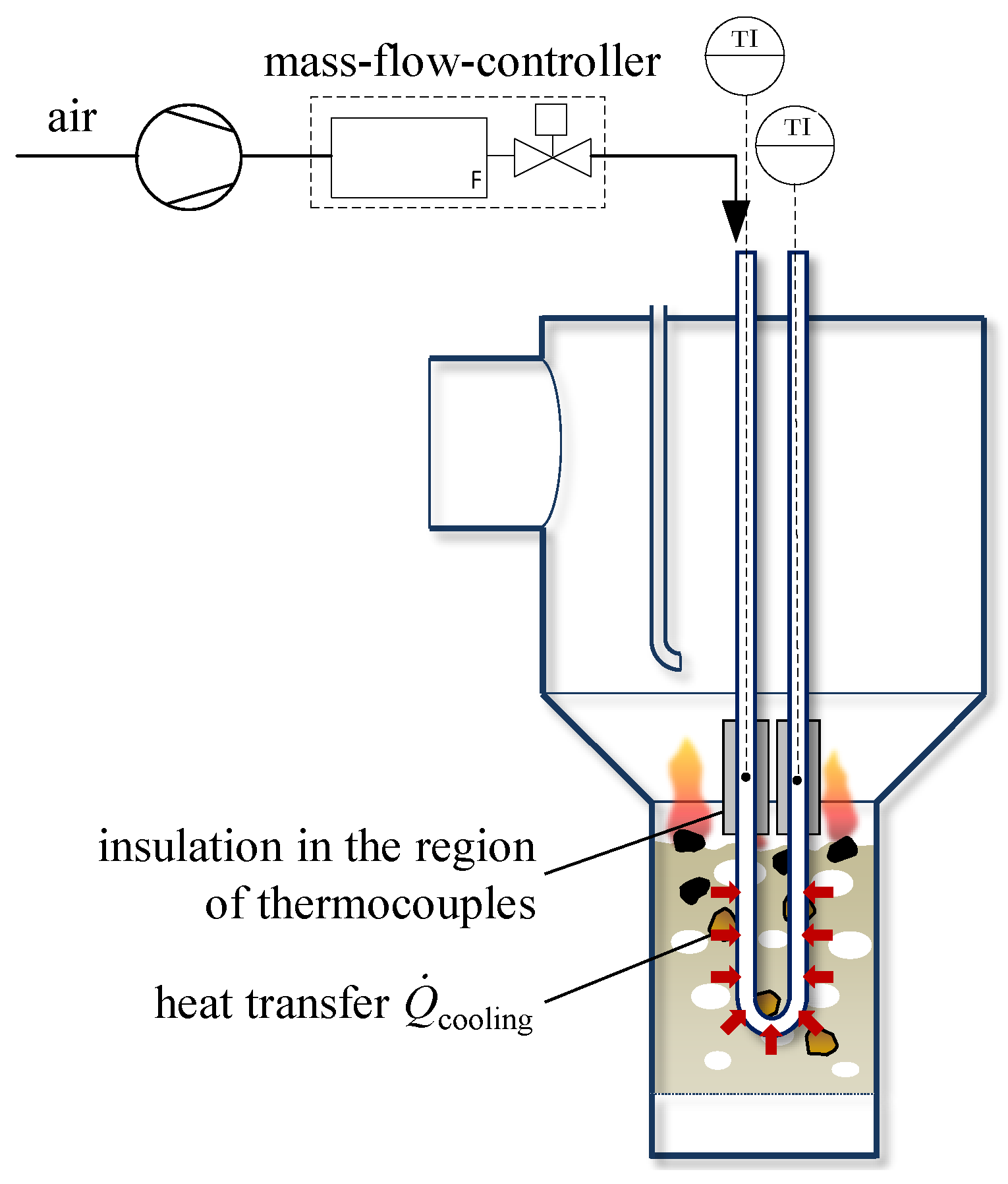
Special emphasis must be given to the electrical bed heater in order to calculate the heat capacity of the fluidised bed . The used heater around the tubular fluidised bed for example has significant heat losses to the ambience. Without proper estimation of this influence, a common measurement of the electrical energy consumption would predict an excessive heat capacity (Equation 10) resulting in a wrong prediction of the heat release efficiency. For this reason, we have to find a correlation between and the actual heat input with the relation . Among several possibilities, a defined cooling at steady-state condition is the most promising approach. Within the presented work, a proper in-bed heat exchanger was used at the preliminary evaluation. An optical access at the top of the fluidised bed reactor allowed an installation of an in-bed cooling coil from the top of the combustion chamber. Air served as cooling medium within the coil, the temperature measurement took place in a heat insulated area in the splashing zone (Figure 5).
With this setup, we consider the following idea that the fluidised bed runs at the electrical heat-up curve as previously described with its heating rate . After starting to cool down the bed with this additional heat-exchanger, the heating rate will be reduced to . According to the previously discussed method to obtain in Equation (10), we can also state that
with a heat flux to the cooling coil according to:
Finally, solving equation
provides a relation to identify the heater efficiency :
5. Results and Discussion
For the electrical bed heater of the 100 fluidised bed combustor, a heat loss of about 11% was determined with this methodology. This results in a correction factor of . Since this value is probably depending on the thermal load and the temperature level, an additional uncertainty of ±10% for the heat input should be taken into account (see Table 2).
For a further interpretation of the below-mentioned results, a brief discussion of the combustion conditions in the freeboard of the furnace is necessary. Each experiment was, due to security reasons, conducted with an additional flow of secondary air to achieve a global fuel-to-air ration of . Especially for combustion conditions with an excess of fuel in the fluidised bed region (), a notable oxidation takes place in the freeboard of the combustion chamber. The heat input due to radiative heat transfer to the surface of the fluidised bed will, in this case, be an additional implicit amount within the heat release efficiency . For a transfer of the achieved data to other fluidised bed combustion chambers, this has to be considered in a critical analysis. As an example, fluidised bed boilers will have water cooled walls, but also the geometrical distance of the secondary air nozzles will usually have a much higher distance to the surface of the fluidised bed compared to this laboratory plant. So the heat transfer conditions in the gas phase will differ between each combustion chamber and have a slight influence on the heat release efficiency. However, the radiative heat transfer from the fluidised bed to the freeboard is implicitly included when calculating the heat capacity of the bed. In the sections of cooling and electrical heating to determine the heat capacity , we find conditions with a nearly constant heat transfer to the freeboard region—in the end this will only affect the gradients of the heat-up and cool-down curve but result in an identical value of . So, cold walls will have an influence on the amount of radiative heat transfer from the flue gas to the surface of the fluidised bed, being the already mentioned specific behaviour of each combustion chamber.
This goes along with the different fluidisation behaviour of small- and large-scale fluidised bed combustion chambers. In a laboratory-scale with usually smaller ratios between the fluidised bed cross section and its height compared to large industrial boilers, bubbles will cover a significantly higher share of the cross sectional area. This influences the transport and mixing of solids and as a result, the distribution of fuel particles within the fluidised bed.
In the following, we describe our results concerning the influence of typical combustion parameters. Table 3 summarizes the different series in our experimental work.
5.1. Influence of Fluidisation Number
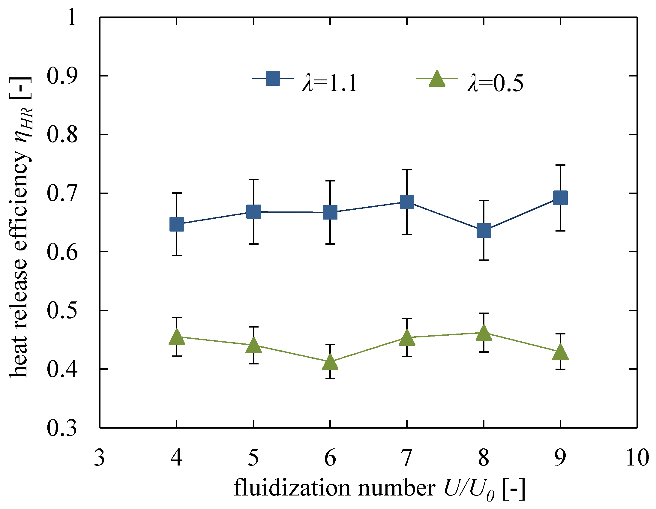
As already indicated in Section 2, the common expectation is that a higher fluidisation velocity leads to an increased mixing of fluidised bed and fuel particles. Especially biomass particles, with their typically low density, should tend to have a longer residence time in the dense zone close to the surface and thus lead to a lower heat release in the fluidised bed. Figure 6 shows several series of measurements along the fluidisation number at different air-to-fuel ratios of and . It appears that an increase of has only little influence on the heat release efficiency. At this point we want to highlight that we had to adjust the fuel input for each test run in order to keep constants air-to-fuel ratios. Otherwise we would have to adjust the grain size of the bed material, which affects the achievable fluidisation ratio due to the test rigs equipment (e.g., limitations of the electrical bed heater or the size of the fuel feeding screw). Taking into account the measurement uncertainties, no significant trend of the heat release with the fluidisation number is visible.
This suggests that the choice of the air-to-fuel ratio will have a higher effect on . In the gasification regime with , due to an obvious lack of combustion air, only 40% to 50% of the fuel energy can be transferred to the dense fluidised bed itself. For nearly stoichiometric conditions at , this value increases to approximately 65%, which is still clearly low compared to an entire theoretical combustion reaction of fuel and air. This seems to be an effect of an insufficient mixing of fuel and air.
In the previous specification of wood pellets [32], the bulk density of wood pellets was given to 1000 to 1400 . During drying and pyrolysis, the fuel particles lose about 85% (see Table 1) of their initial weight at nearly constant size [34]. Finally, this means that the density of the remaining fixed carbon lies in the range of 150 to 210 . According to [35], relation
can estimate the porosity of the dense zone of fluidised bed depending on the well-known dimensionless Reynolds and Archimedes numbers. For the density of the fluidised bed being the sum of the densities of solids and gas phase according to
one obtains values of for the range of .
This means that, according to the Archimedes principle, the particles must tend to accumulate in the upper region of the fluidised bed. Obviously, the high fluidisation ratio avoids the effect of having mainly floating particles at the surface of the fluidised bed. Unfortunately, due to an arising non-isothermal behaviour in the bed region of the lab-scale plant, it is not possible to set a clearly lower fluidisation ratio for the experiments as it occurs in large scale fluidised bed boilers with coarser bed materials. An application of this procedure for the given combustion chamber would require at least an extended air pre-heater to decrease the temperature difference between fluidised bed and primary air. This would improve the fluidisation in the lower bed region towards a uniform temperature distribution.
For further measurements, fluidisation numbers of and were investigated, as they are particularly suitable for a trade-off between isothermal behaviour, duration and particle emissions in the presented experimental setup.
5.2. Influence of Fluidised Bed Temperature
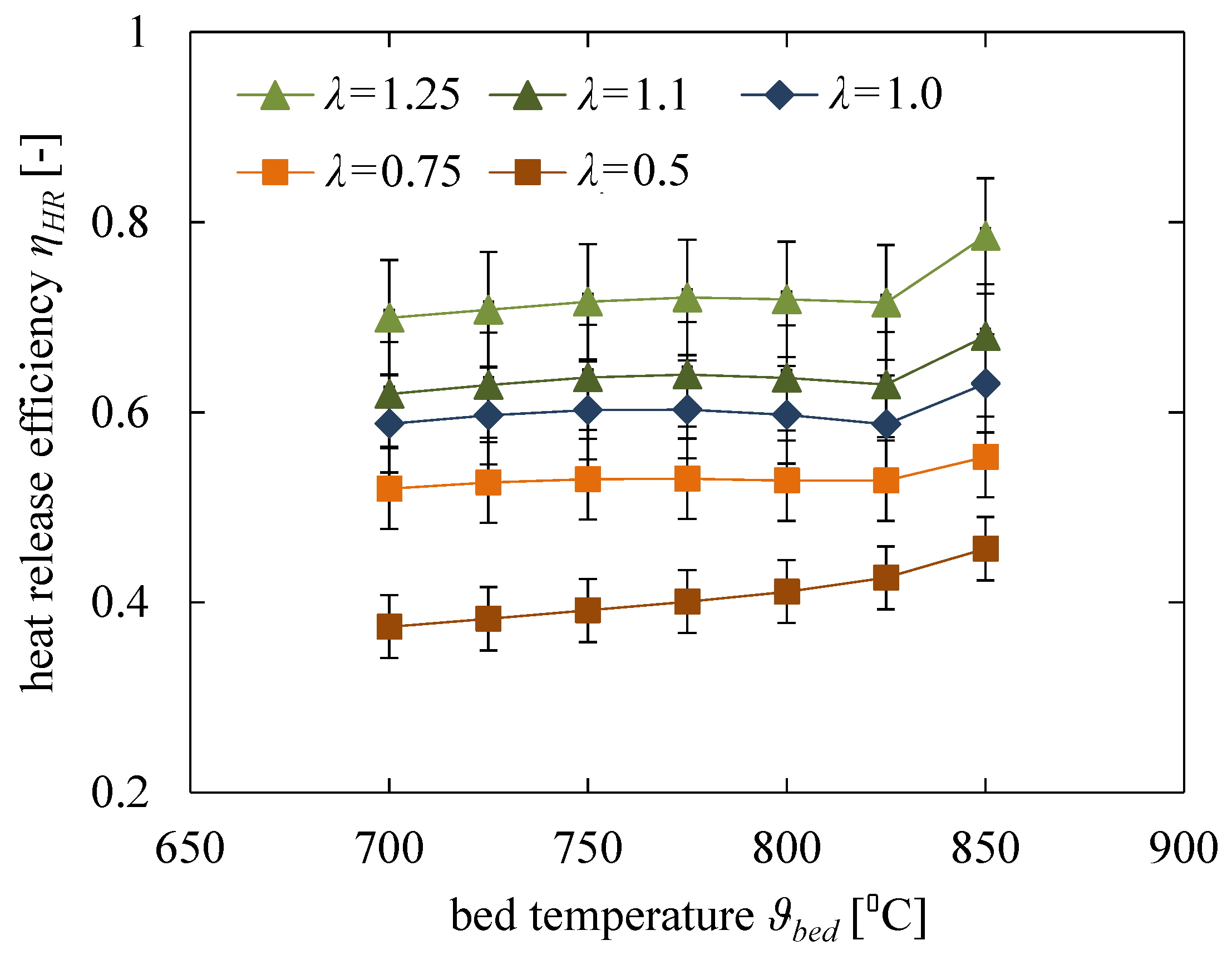
Concerning fluidised bed temperature , different reaction kinetics will influence some gas-phase conversion mechanisms. A higher temperature level leads to a slightly increased combustion reaction of volatiles or carbon-monoxide with air especially before these species are leaving the fluidised bed zone. This could also probably influence the heat release due to an increased conversion rate. Experiments focusing on this effect were performed also for several fuel-to-air ratios at a fluidisation number of , as presented in Figure 7.
The results show also no significant influence of the bed temperature on the heat release efficiency along the temperature range of 700 °C to 850 °C. Some occasional trends to an increased heat release are mainly in the scale of the measurement uncertainty. Again, the strong influence of the air-to-fuel ratio is apparent in this series, namely the steady increase of the heat release with an increasing amount of air up to .
For further measurements, it can be stated that a desired target temperature for the heat release efficiency measurements of 800 °C is representative for the common operating range of a fluidised bed combustor.
5.3. Influence of Air-to-Fuel Ratio and Fuel Properties
In this sequence, three different fuels, namely wood pellets, lignite and polyethylene (see Table 1) at air-to-fuel ratios of , were used.
In this series, the heat release efficiency shows a steady increase along the fuel-to-air ratio from about 40% () up to 90% (). For stoichiometric conditions , lignite provides the highest heat release efficiency compared to the other fuels. In contrast, wood pellets dominate in the gasifier mode of . Compared with wood pellets, polyethylene granules tend to have a 10% reduced heat release efficiency. As already considered in Section 5.1, even in this series, no significant influence of the fluidisation number could be detected. Indeed, for , the results show mostly a higher heat release; however, the difference is the order of magnitude of the Gaussian error propagation. For a better transparency, the error bars are not shown in Figure 8, but can be easily transferred from the already presented data. For more precise results, multiple measurements would have to be advised in the future.
Compared with the influence of the fluidisation number and the fluidised bed temperature it can be summarised that the air-to-fuel ratio is the decisive parameter for a higher heat release efficiency. For operating conditions with an excess of fuel, it is obvious that the conversion is limited, whereas for a sufficient air availability, an imperfect mixing seems to be responsible for an incomplete heat release efficiency.
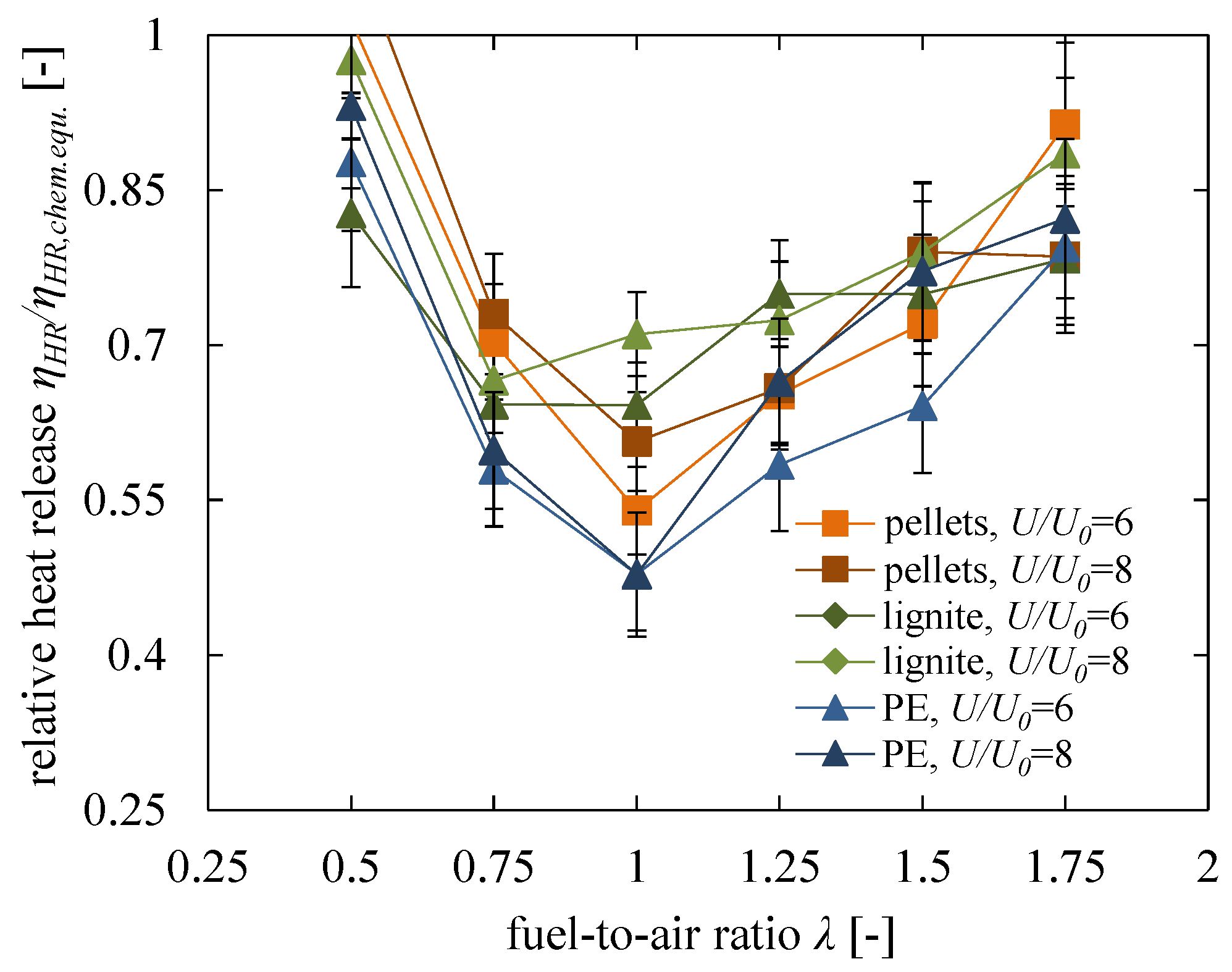
This can be confirmed by regarding the heat release efficiency relative to the theoretical heat of the reaction at the chemical equilibrium . This represents the thermodynamic limit of the combustion reaction for fuel rich conditions. The authors used FactSage to calculate the gaseous components at the chemical equilibrium for the specific fuel composition and temperatures. In this assumption, the fixed carbon is fully converted to gaseous species. This is in accordance with the idea of having steady-state conditions with no further accumulation of fixed carbon in the reactor. Finally, after calculating the remaining heating value of this gas composition at the chemical equilibrium , one can relate it to the heating value of the solid fuel :
Figure 9 shows this ratio for the previously mentioned series with the dependency of the fuel-to-air ratio. For conditions with twice as much fuel () than the stoichiometric ratio, the relative heat release is nearly 100%. In this case, even for incomplete mixing, each oxygen molecule will get in contact with the excess fuel components. The value slightly above 100% results from the measurement uncertainty, but also from an imprecise ultimate analysis or a fluctuating moisture content. Especially the radiative heat transfer from the post-combustion in the freeboard will have its influence too. Then, the relative heat release decreases along the fuel-to-air ratio with a minimum of at .
For lean combustion conditions, which of course allow a complete combustion, the relative heat release is equivalent to the measured values. In this range, the relative heat release rises towards its maximum of 100% for . The reason for this behaviour can be found in the limited mixing of fuel and combustion air in the upper region of a fluidised bed compared in comparison to gas burners. A nearly complete combustion requires either a strong fuel or air excess in order to ensure a sufficient mixing in the limited residence time within the fluidised bed. An increased volatile content of the fuel enhances this behaviour, as lignite shows the highest relative heat release at compared to the lowest value of polyethylene. In this case, an increased amount of pyrolysis products leaves the fluidised bed unburnt. However, the char conversion at fluidised bed temperatures of 800 °C is mainly dominated by the exothermic reaction with oxygen. So the heterogeneous reaction of carbon to carbon-monoxide can only take place in the presence of oxygen with a release of energy. Though the oxidation to the final product carbon-dioxide could happen in the freeboard area, at least the first step to carbon-monoxide has to take place in the fluidised bed zone.
5.4. Comparison of Results with Scala’s Model
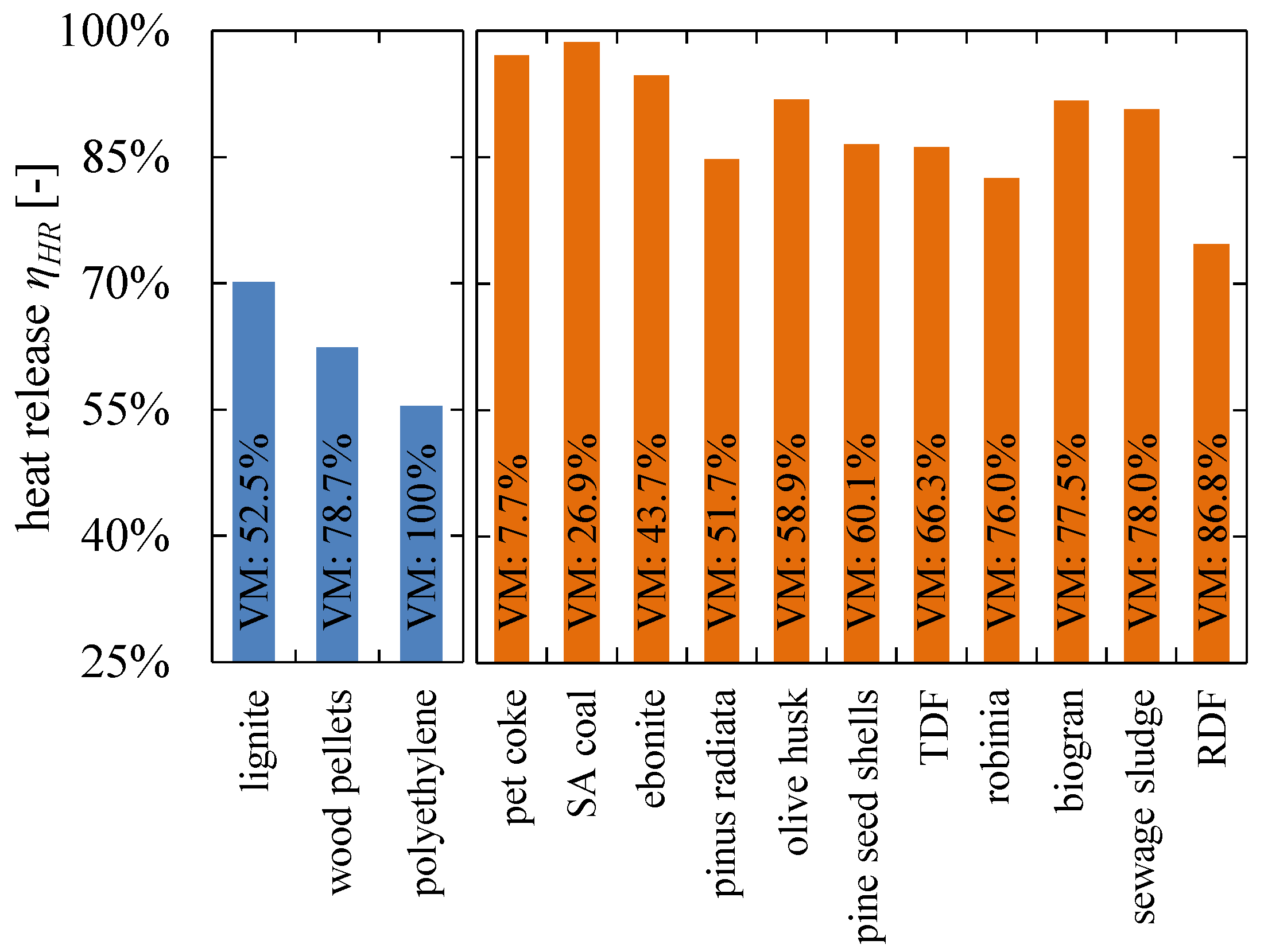
Finally, we compare our results with the already described model from Scala et al. [24,25] in Section 2. The findings from the presented work also allow a comparison with their modelled results for different fuel in the context of varying volatile content. As their data is given for a fuel-to-air ratio of , the previously shown experimental results were interpolated in a proper way to arrange them in common chart (Figure 10).
Both series show an according decline of the heat release efficiency with an increasing volatile matter of the fuel. This means that both approaches describe the influence of the volatile content. However, our experimental results lie in the range from 55% to 70%, while Scala’s model provides results in the range of 73% to 98%. So, compared to our results, the approach of Scala shows a heat release efficiency up to nearly 100%, especially for fossil fuels with a dominating content of fixed carbon. With the presented experimental methodology, this nearly complete heat release would need a high excess of air at .
One possibility for these differences in Scala’s model and our measurements could be the two-dimensional distribution of particles within the cross-section of a fluidised bed. Scala’s approach is a one-dimensional formulation as a function of the height and does not consider a non-uniform spatial location of fuel particles. In this case, maybe the formation of fuel-rich and lean combustion zones leading to a reduced heat release in the upper section of the fluidised bed are under-represented. Otherwise, the shape of our combustion chamber might influence the gained heat release efficiencies. The different ratio of cross-section and height between the lab-scale reactor with higher wall effects and an industrial boiler will significantly influence the bubble growth and the mixing near the surface of the fluidised bed.
Further data governed by their model in future work would be highly interesting to compare, as well as the forecast of all other combustion parameters.
6. Conclusions
This work presents a methodology for the experimental evaluation of the heat release efficiency in bubbling fluidised bed boilers. The motivation for the development of this procedure is the fact that especially biogenic fuels tend to accumulate in the upper section near the surface of the fluidised bed. During the combustion process, this will lead to a release of volatile or still unburnt species in the freeboard region. As a consequence, their heat of combustion when burning above the fluidised bed will not be released in the bed region and affect the thermal management of a bubbling fluidised bed combustion chamber.
The presented method is based on transient temperature profiles recorded on a lab-scale fluidised bed combustor in several sequences with and without fuel feeding. Afterwards, a mathematical derived equation allows the calculation of the heat release efficiency. Special focus lies on the determination of the reactors’ heat capacity. An appropriate approach is, for example, a defined heating or cooling with corresponding temperature gradients of the fluidised bed.
Measurements were performed with different fuels for fluidised bed temperatures of 700 °C to 850 °C, fuel-to-air ratios in the range of and fluidisation ratios of 6 and 8. Altogether, the obtained results allow several conclusions:
- The influence of the fluidised bed temperature has a minor effect on the heat release efficiency.
- Also, the trend to an increased heat release efficiency with an increasing fluidisation ratio is mainly in the scale of the measurement uncertainty. Unexpectedly, this does not fully confirm the common opinion, that the better mixing at higher fluidisation ratios will support the complete burnout of fuel particles inside the fluidised bed. However, the results so far do not provide enough information for a full understanding of this effect. Further tests with a detailed focus on the influence of fuel and especially the density of the bed material (e.g., olivine) will have to follow for a better understanding.
- A significant influence was found for the fuel-to-air ratio . As an operation at can of course not provide a heat release of 100%; a high fuel excess of is necessary to reach the maximum possible heat release according to the thermal equilibrium. A similar trend was found for , where only a high excess of air can ensure a nearly entire heat release within the fluidised bed. For stoichiometric conditions, a fuel-depending heat release efficiency of was obtained, which can be explained with non-ideal mixing of fuel and oxygen in the remaining residence time before leaving the dense fluidised bed.
Author Contributions
D.M. and J.K. conceived and developed the methodology; D.M. and T.P. performed the measurements; D.M. analysed the results; D.M., T.P. and J.K. wrote the paper. All authors have read and agreed to the published version of the manuscript.
Funding
This research received no external funding.
Conflicts of Interest
The authors declare no conflict of interest.
Abbreviations
The following abbreviations are used in this manuscript:
| BFB | bubbling fluidised bed |
| CFB | circulating fluidised bed |
| PE | polyethylene |
| Ar | Archimedes number [-] |
| specific heat capacity of the air [] | |
| specific heat capacity of the flue gas [] | |
| particle size [m] | |
| porosity [-] | |
| in-bed heat release efficiency of the BFB combustion [-] | |
| heating value of the fuel [] | |
| air-to-fuel ratio [-] | |
| fuel mass flow [] | |
| air mass flow [] | |
| flue gas mass flow [] | |
| heat capacity of the dense fluidised bed [] | |
| heat input in the dense fluidised bed [kW] | |
| fuel heat input [kW] | |
| heat losses [kW] | |
| electrical bed heater input [kW] | |
| electrical input [kW] | |
| Re | Reynolds number [-] |
| density of the dense fluidised bed phase [] | |
| density of solid phase [] | |
| density of gaseous phase [] | |
| t | time [s] |
| temperature of the fluidised bed [°C] | |
| temperature of the air [°C] | |
| temperature of the flue gas [°C] | |
| U | fluidisation velocity [] |
| minimum fluidisation velocity [] | |
| fluidisation number [-] |
References
- Koornneef, J.; Junginger, M.; Faaij, A. Development of fluidized bed combustion-An overview of trends, performance and cost. Prog. Energy Combust. Sci. 2007, 33, 19–55. [Google Scholar] [CrossRef] [Green Version]
- Werther, J.; Holighaus, R. Wirbelschicht-Technologie: Neuentwicklungen für Kraftwerkstechnik und Umweltschutz. Chem. Ing. Tech. 1978, 50, 662–669. [Google Scholar] [CrossRef]
- Leckner, B. Fluidized bed combustion: Mixing and pollutant limitation. Prog. Energy Combust. Sci. 1998, 24, 31–61. [Google Scholar] [CrossRef]
- Schu, R.; Leithner, R. Mehrstufige Dampfüberhitzung Effizienzsteigerung von EBS-, Biomasse-und Solarthermiekraftwerken. In Berliner Abfallwirtschafts-und Energiekonferenz; Thomé-Kozmiensky, K., Beckmann, M., Eds.; TK Verlag: Neuruppin, Germany, 2008. [Google Scholar]
- Winter, F.; Szentannai, P. Brennstoffmix in Wirbelschichtfeuerungen: Status und Entwicklungstendenzen. In Proceedings of the 6th Internationale Energiewirtschaftstagung an der TU Wien, Vienna, Austria, 11–13 February 2009. [Google Scholar]
- Khan, A.A.; de Jong, W.; Jansens, P.J.; Spliethoff, H. Biomass combustion in fluidized bed boilers: Potential problems and remedies. Fuel Process. Technol. 2009, 90, 21–50. [Google Scholar] [CrossRef]
- Plankenbü, T.; Müller, D.; Karl, J. Slagging Prevention and Plant Optimisation by Means of Numerical Simulation. In Proceedings of the 25th European Biomass Conference & Exhibition, Stockholm, Sweden, 12–15 June 2017. [Google Scholar]
- Plankenbühler, T.; Müller, D.; Karl, J. Influence of Fine Fuel Particles on Ash Deposition in Industrial-Scale Biomass Combustion: Experiments and Computational Fluid Dynamics Modeling. Energy Fuels 2019, 33, 5911–5917. [Google Scholar] [CrossRef]
- Gatternig, B.; Karl, J. Investigations on the mechanisms of ash-induced agglomeration in fluidized-bed combustion of biomass. Energy Fuels 2015, 29, 931–941. [Google Scholar] [CrossRef]
- Gatternig, B.; Karl, J. The influence of particle size, fluidization velocity and fuel type on ash-induced agglomeration in biomass combustion. Front. Energy Res. 2014, 2, 1–12. [Google Scholar] [CrossRef] [Green Version]
- Müller, D.; Karl, J. Biomass CHP with micro-fluidized-bed combustion. In Proceedings of the 21st European Biomass Conference & Exhibition, Copenhagen, Denmark, 3–7 June 2013. [Google Scholar]
- Rowe, P.N.; Nienow, A.W. Particle mixing and segregation in gas fluidised beds. A review. Powder Technol. 1976, 15, 141–147. [Google Scholar] [CrossRef]
- Wu, S.Y.; Baeyens, J. Segregation by size difference in gas fluidized beds. Powder Technol. 1998, 98, 139–150. [Google Scholar] [CrossRef]
- dos Santos, F.; Goldstein, L. Experimental aspects of biomass fuels in a bubbling fluidized bed combustor. Chem. Eng. Process. Process Intensif. 2008, 47, 1541–1549. [Google Scholar] [CrossRef]
- Gómez-Barea, A.; Ollero, P.; Leckner, B. Optimization of char and tar conversion in fluidized bed biomass gasifiers. Fuel 2013, 103, 42–52. [Google Scholar] [CrossRef]
- Wirsum, M.; Fett, F.; Iwanowa, N.; Lukjanow, G. Particle mixing in bubbling fluidized beds of binary particle systems. Powder Technol. 2001, 120, 63–69. [Google Scholar] [CrossRef]
- Zhang, Y.; Jin, B.; Zhong, W. Experimental investigation on mixing and segregation behavior of biomass particle in fluidized bed. Chem. Eng. Process. Process Intensif. 2009, 48, 745–754. [Google Scholar] [CrossRef]
- Shen, L.; Xiao, J.; Niklasson, F.; Johnsson, F. Biomass mixing in a fluidized bed biomass gasifier for hydrogen production. Chem. Eng. Sci. 2007, 62, 636–643. [Google Scholar] [CrossRef]
- Bruni, G.; Solimene, R.; Marzocchella, A.; Salatino, P.; Yates, J.G.; Lettieri, P.; Fiorentino, M. Self-segregation of high-volatile fuel particles during devolatilization in a fluidized bed reactor. Powder Technol. 2002, 128, 11–21. [Google Scholar] [CrossRef]
- Cui, H.; Grace, J.R. Fluidization of biomass particles: A review of experimental multiphase flow aspects. Chem. Eng. Sci. 2007, 62, 45–55. [Google Scholar] [CrossRef]
- Li, L.; Duan, L.; Yang, Z.; Zhao, C. Pressurized oxy-fuel combustion characteristics of single coal particle in a visualized fluidized bed combustor. Combust. Flame 2020, 211, 218–228. [Google Scholar] [CrossRef]
- Sette, E.; Berdugo Vilches, T.; Pallarès, D.; Johnsson, F. Measuring fuel mixing under industrial fluidized-bed conditions - A camera-probe based fuel tracking system. Appl. Energy 2016, 163, 304–312. [Google Scholar] [CrossRef]
- Köhler, A.; Pallarès, D.; Johnsson, F. Modeling Axial Mixing of Fuel Particles in the Dense Region of a Fluidized Bed. Energy Fuels 2020, 34, 3294–3304. [Google Scholar] [CrossRef]
- Scala, F.; Salatino, P. Modelling fluidized bed combustion of high-volatile solid fuels. Chem. Eng. Sci. 2002, 57, 1175–1196. [Google Scholar] [CrossRef]
- Scala, F.; Chirone, R. Fluidized bed combustion of alternative solid fuels. Exp. Therm. Fluid Sci. 2004, 28, 691–699. [Google Scholar] [CrossRef]
- Ottmann, M. Verbrennung Biogener Brennstoffe in Stationären Wirbelschichtfeuerungen. Ph.D. Thesis, Technische Universität München, München, Germany, 2007. [Google Scholar]
- Reschmeier, R.; Roveda, D.; Müller, D.; Karl, J. Pyrolysis kinetics of wood pellets in fluidized beds. J. Anal. Appl. Pyrolysis 2014, 108, 117–129. [Google Scholar] [CrossRef]
- Reschmeier, R.; Karl, J. Experimental study of wood char gasification kinetics in fluidized beds. Biomass Bioenergy 2016, 85, 288–299. [Google Scholar] [CrossRef]
- Mastellone, M.L.; Perugini, F.; Ponte, M.; Arena, U. Fluidized bed pyrolysis of a recycled polyethylene. Polym. Degrad. Stab. 2002, 76, 479–487. [Google Scholar] [CrossRef]
- Mastral, F.J.; Esperanza, E.; García, P.; Juste, M. Pyrolysis of high-density polyethylene in a fluidised bed reactor. Influence of the temperature and residence time. J. Anal. Appl. Pyrolysis 2002, 63, 1–15. [Google Scholar] [CrossRef]
- Baumhakl, C. Substitute Natural Gas Production with direct Conversion of Higher Hydrocarbons. Ph.D. Thesis, Friedrich-Alexander-Universität Erlangen-Nürnberg, Erlangen, Germany, 2014. [Google Scholar]
- Prüfung Fester Brennstoffe—Presslinge aus Naturbelassenem Holz—Anforderungen und Prüfung—Fassung DIN 51731; Beuth: Berlin, Germany, 1996.
- Annamalia, K.; Sweeten, J.M.; Ramalingam, S.C. Technical Notes: Estimation of Gross Heating Values of Biomass Fuels. Trans. ASAE 1987, 30, 1205–1208. [Google Scholar] [CrossRef]
- Paulauskas, R.; Džiugys, A.; Striugas, N. Experimental investigation of wood pellet swelling and shrinking during pyrolysis. Fuel 2015, 142, 145–151. [Google Scholar] [CrossRef]
- Michel, W. (Ed.) Wirbelschichttechnik in der Energiewirtschaft; Deutscher Verlag für Grundstoffindustrie GmbH: Leipzig, Germany, 1992. [Google Scholar]
Figure 1.
Energy balance of a bubbling fluidised bed combustion chamber.
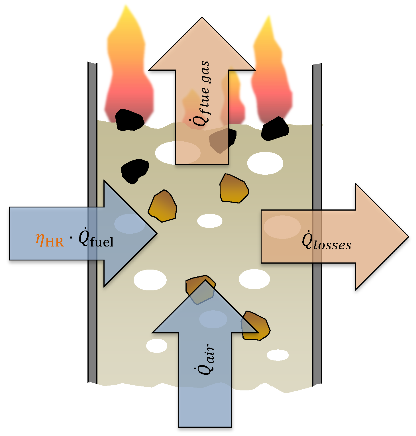
Figure 2.
Time-depending combustion conditions for the transient sequence in the presented methodology.
Figure 2.
Time-depending combustion conditions for the transient sequence in the presented methodology.
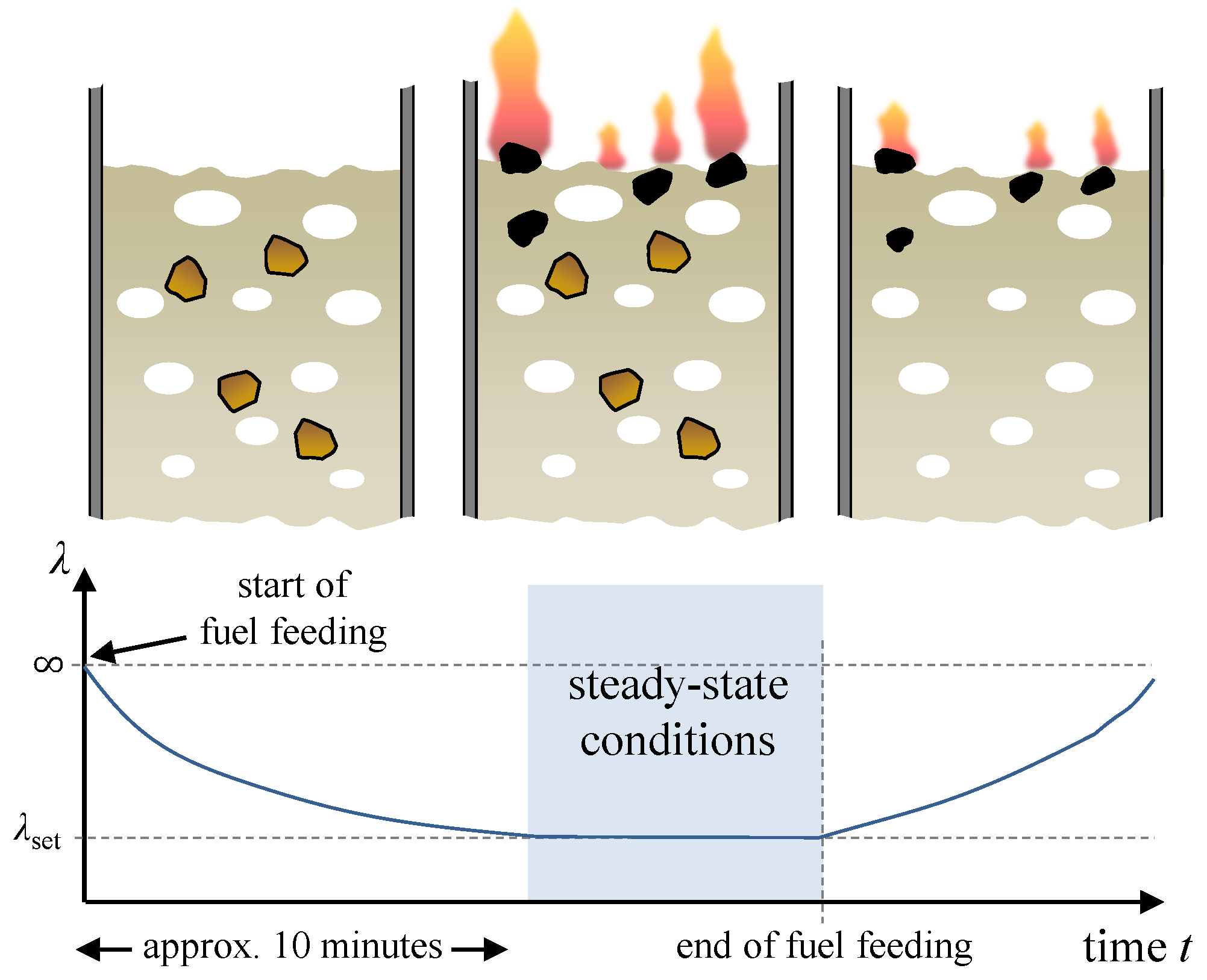
Figure 3.
Experimental implementation for a determination of the heat release efficiency within a lab-scale fluidised bed combustion plant.
Figure 3.
Experimental implementation for a determination of the heat release efficiency within a lab-scale fluidised bed combustion plant.

Figure 4.
100 bubbling fluidised bed combustor at the Chair of Energy Process Engineering.

Figure 5.
Installation of an in-bed cooling coil for a more precise determination of the fluidised bed’s heat capacity.
Figure 5.
Installation of an in-bed cooling coil for a more precise determination of the fluidised bed’s heat capacity.

Figure 6.
Influence of the fluidisation ratio on the heat release efficiency within a fluidised bed combustion (fuel: wood pellets, 800 °C ).
Figure 6.
Influence of the fluidisation ratio on the heat release efficiency within a fluidised bed combustion (fuel: wood pellets, 800 °C ).

Figure 7.
Influence of the bed temperature on the heat release efficiency within a fluidised bed combustion (fuel: wood pellets, ).
Figure 7.
Influence of the bed temperature on the heat release efficiency within a fluidised bed combustion (fuel: wood pellets, ).

Figure 8.
Influence of the fuel-to-air ratio on the heat release efficiency within a fluidised bed combustion ( 800 °C).
Figure 8.
Influence of the fuel-to-air ratio on the heat release efficiency within a fluidised bed combustion ( 800 °C).
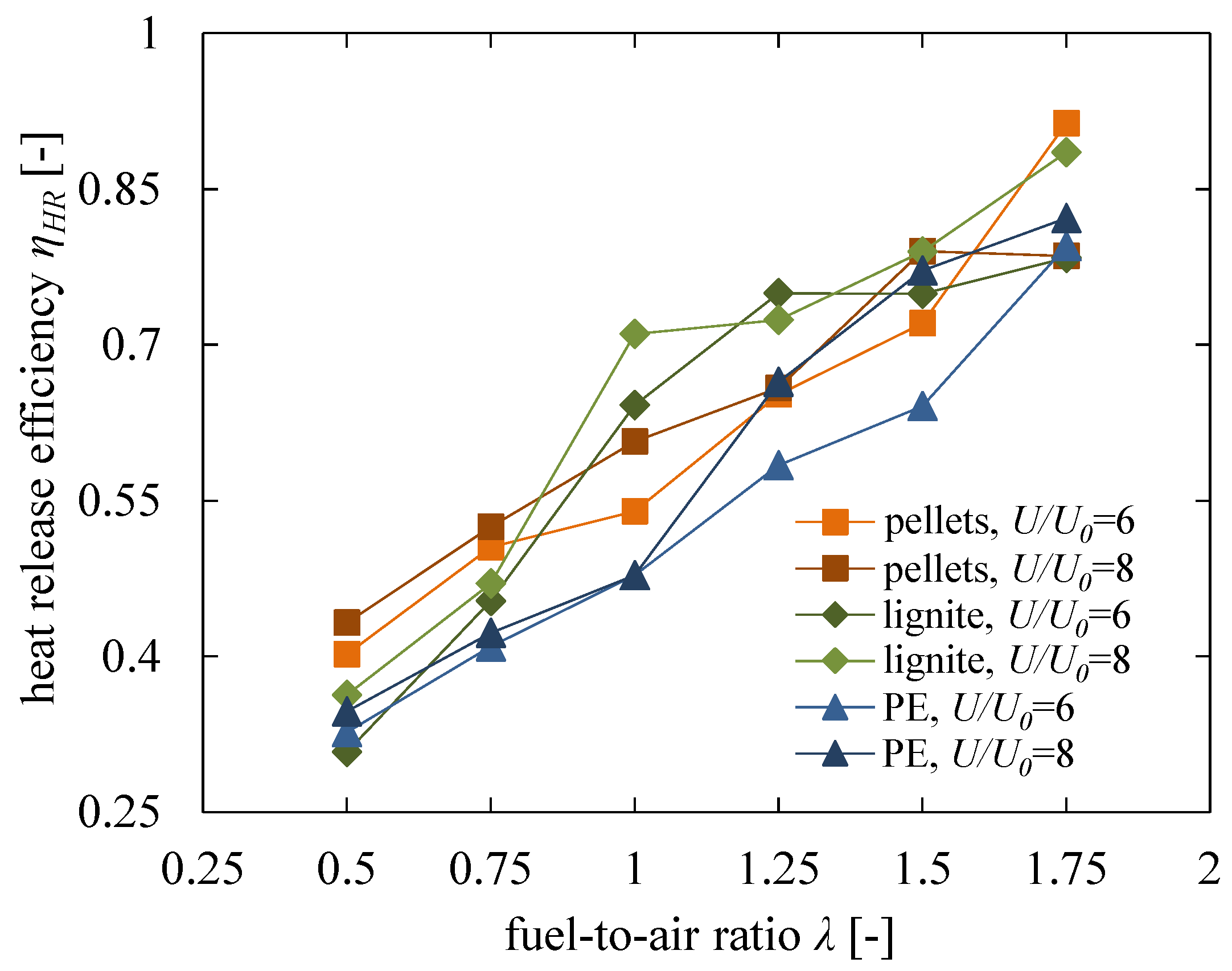
Figure 9.
Relative heat release efficiency correlated to its maximum value according to the chemical equilibrium 800 °C.
Figure 9.
Relative heat release efficiency correlated to its maximum value according to the chemical equilibrium 800 °C.

Figure 10.
Comparison of the experimental results from the presented work with the modelled data from Scala [25] for different fuels with varying volatile contents (own results interpolated for ).
Figure 10.
Comparison of the experimental results from the presented work with the modelled data from Scala [25] for different fuels with varying volatile contents (own results interpolated for ).


| Property | Wood Pellets 1) | Lignite | Poly-Ethylene 2) |
|---|---|---|---|
| c [-%] | 46.8 | 53.6 | 85.6 |
| h [-%] | 5.7 | 3.9 | 14.4 |
| o [-%] | 40.1 | 19.2 | 0 |
| n [-%] | 0 | 0.6 | 0 |
| s [-%] | 0 | 0.4 | 0 |
| w [-%] | 6.9 | 19.0 | 0 |
| ash [-%] | 0.5 | 3.5 | 0 |
| volatile matter [-%] | 78.7 | 42.0 | 100 |
| fixed carbon [-%] | 14.0 | 35.5 | 0 |
| [] | 17.1 | 19.8 | 43.3 |
| particle size [] | 6 | 4–12 | 4.5 |
| density [] | 1000–1400 | n/a | 950 |
1) Own analysis; density and size from specification [32]. 2) Composition according to the chemical composition of the monomer ; density and size from datasheet of LyondellBasell.
Table 2.
Uncertainties of each variable during the evaluation of the heat release efficiency.
| Variable | (Relative) Uncertainty |
|---|---|
| fuel mass flow | 5% 1) |
| air mass flow | 0.6% 2) |
| heating value | 2% 3) |
| specific heat capacity flue gas | 3% |
| specific heat capacity air | 1% |
| fluidised bed temperature | 2.1% 4) |
| temperature gradients , and | 2% 5) |
| electrical bed heater | 10% 6) |
1) Empirical value of uncertainties for calibration of fuel feeding screws. 2) Calibration certificate by the manufacturer. 3) Uncertainty of Boie formula [33]. 4) Fluidised bed temperature is the mean value of two sensors. This reduces the common uncertainty of a thermocouples (3%) by a factor of . 5) An automatic data processing is assumed to have an maximum error of 2% for a sufficient period. Any temperature offset of a thermocouple or an A/D-converter do not have to be considered. 6) Estimated heat losses of a radiation furnace at elevated temperatures.
Table 3.
Brief overview of the different series for the experimental work.
| Influence of | Variation of | Constant Parameters |
|---|---|---|
| fluidisation number | 800 °C, & , wood pellets | |
| bed temperature | 700 °C °C | , , wood pellets |
| fuel properties | wood pellets, lignite, polyethylene at | 800 °C, , |
© 2020 by the authors. Licensee MDPI, Basel, Switzerland. This article is an open access article distributed under the terms and conditions of the Creative Commons Attribution (CC BY) license (http://creativecommons.org/licenses/by/4.0/).
Share and Cite
MDPI and ACS Style
Müller, D.; Plankenbühler, T.; Karl, J. A Methodology for Measuring the Heat Release Efficiency in Bubbling Fluidised Bed Combustors. Energies 2020, 13, 2420. https://doi.org/10.3390/en13102420
AMA Style
Müller D, Plankenbühler T, Karl J. A Methodology for Measuring the Heat Release Efficiency in Bubbling Fluidised Bed Combustors. Energies. 2020; 13(10):2420. https://doi.org/10.3390/en13102420
Chicago/Turabian StyleMüller, Dominik, Thomas Plankenbühler, and Jürgen Karl. 2020. "A Methodology for Measuring the Heat Release Efficiency in Bubbling Fluidised Bed Combustors" Energies 13, no. 10: 2420. https://doi.org/10.3390/en13102420
Note that from the first issue of 2016, this journal uses article numbers instead of page numbers. See further details here.