Multi-Horizon Dependence between Crude Oil and East Asian Stock Markets and Implications in Risk Management

Abstract

This paper examines the dynamic dependence structure of crude oil and East Asian stock markets at multiple frequencies using wavelet and copulas. We also investigate risk management implications and diversification benefits of oil-stock portfolios by calculating and comparing risk and tail risk hedging performance. Our results provide strong evidence of time-varying dependence and asymmetric tail dependence between crude oil and East Asian stock markets at different frequencies. The level and fluctuation of their dependencies increase as time scale increases. Furthermore, we find the time-varying hedging benefits differ at investment horizons and reduced over the long run. Our results suggest that crude oil could be used as a hedge and safe haven against East Asian stock markets, especially in the short- and mid-term.

1. Introduction

Crude oil remained the world’s leading fuel, accounting for 33.6% of global energy consumption in 2018 and BP’s Statistical Energy Outlook suggests that it will continue to play a similar role until 2035. The influence of oil prices has become crucial for world economic development. It is fair to argue that oil remains to be one of the biggest drivers of the global economy. Furthermore, with the financialization of commodity markets, oil price not only have been concerned with macroeconomic factors, but also have become a critical part in financial field. Since the correlations between commodity and stock markets are low, crude oil has become an alternative investment tool for international portfolio diversification [1,2]. Analyzing price relationships between crude oil and stock markets is an essential topic of modern finance, especially in derivative pricing, portfolio allocation and risk management.

In this paper, we investigate the dynamic dependence between crude oil and East Asian stock markets. Many literatures have examined the oil-stock relationship [3,4,5,6,7,8,9] for many developed countries, while the problem of how they work on the developing region such as East Asia attracts less attention. In fact, this subject is interesting and important. Over the previous decades, East Asian has experienced the fastest economic growth in the world and become one of the three core economic regions [10]. Its miraculous economic growth and dynamism has attracted increasing attention of business interest and academic research [11,12]. The demand for oil of East Asia has been increasing for years. Additionally, East Asia is highly susceptible to oil shocks, for example, the 2003 Iraq war and the 2006 OPEC cut agreement, since the majority of East Asian oil imports are from the Middle East, and there has been no regional mechanism to stockpile emergency petroleum in East Asia [13]. Therefore, crude oil price fluctuations influenced East Asian economies to a larger extent than the developed countries. On the other hand, the hedging benefits from portfolio diversification is a major subject in the financial literatures. Investors make great efforts to improve the risk-return tradeoff of their portfolios in times of financial crises. Specifically, investors look to a more defensive diversification strategy by choosing alternative assets such as crude oil. These particularities of East Asia have therefore attracted great attentions from global investors, policy makers and portfolio managers. Understanding the dynamic dependence between crude oil and East Asian stock markets is very important to those interested in global asset allocation and risk management.

Although the idea of utilizing crude oil as portfolio diversification tool attracted much attention, we found no consensus regarding their relationship. For example, in [14], the authors suggest that there is a negative relationship between oil price shocks and international equity returns. In [15], the authors conclude that oil is an almost perfect diversification tool for stocks, since their correlations are low, or even negative. However, in [16], the authors documents that an increase in oil prices exhibits a positive effect on the equity returns. The decreasing benefit of adding crude oil to stock portfolios over the past ten years is find in [4].

Another limitation of the literatures is that they are restricted to one or, at most, two aspects–the short and long term, paying little attention to the specific dependence structure between crude oil and stock markets by considering multiple frequencies. In this paper, we fill this gap and contribute to current literatures in two ways.

First, this research is novel in that, we model the oil-stock relationship using wavelets and copulas, which can provide information on both dependence and tail dependence at different frequencies, as discussed in [17,18]. This unique setting provides information on both the over-time and cross-scale dynamic dependences, which are crucial for portfolio allocation and risk management.

The second way we contribute to literature is that we investigate the implications of their dependence and tail dependence for risk management purpose at different investment horizons. More precisely, we investigate the time-varying risk and downside risk hedging performance by calculating and comparing the variance and expected shortfall of oil-stock portfolios to stock-only portfolios at different frequencies. The empirical results provide strong evidence that oil is an effective hedge and safe haven against East Asian stock markets.

The remainder of the article is organized as follows. In Section 2, we introduce the model specification, including the marginal distributions, the wavelet transform, as well as the conditional copula functions. Section 3 briefly describes our data. In Section 4, we present and discuss our empirical results. In Section 5, we investigate risk management implications of oil-stock dependence and tail dependence at different investment horizons. Section 6 concludes.

2. Model Specification

Our model combines the wavelet transform analysis and the conditional copula functions to examine the relationship of the markets. Specifically, we utilize the wavelet transform to decompose the standardized shocks obtained from marginal models into time series at different frequency, and then employ the conditional static and dynamic copula functions to capture their constant and dynamic interdependence and tail dependence across different time horizons respectively.

2.1. Marginal Distribution Models

We first model the marginal distribution for each asset market. We assume that the autoregressive-generalized autoregressive conditional heteroskedasticity (AR-GARCH) type models for the conditional mean and variance. The equation of the return series ($y_{i,t}$) is as follows:

$$y_{i,t}={\mu }_i\left(y_{i,t-p}, \varphi \right)+{\sigma }_{i,t}\left(y_{i,t-1}, \mathsf{\theta }\right)z_{i,t},z_{i,t}|{ℱ}_{t-1}~F_i\left(0,1\right)$$

(1)

where ${\mu }_i$ is the conditional mean, ${\sigma }_{i,t}$ is the conditional variance, $z_{i,t}$ is the standardized residual, and ${ℱ}_{t-1}$ is the information set. $\varphi$ and θ are the vector of parameters.

We use the AIC and BIC to determine the order of mean equation (p) and consider the volatility models in the Glosten–Jagannathan–Runkle-generalized autoregressive conditional heteroscedasticity (GJR-GARCH) (1, 1, 1) process [19] as follows:

$$y_{i,t}= {\varphi }_{0,i}+{\displaystyle \sum }{\varphi }_{p,i}{y}_{i,t-p}+{\epsilon }_{i,t}, i=1,\dots ,n,$$

(2)

$${\epsilon }_{i,t}=z_{i,t}{\sigma }_{i,t}, z_{i,t}|{ℱ}_{t-1}~\left(0,1\right)$$

$${\sigma }_{i,t}^2={\omega }_i+{\beta }_i{\sigma }_{i,t-1}^2+{\alpha }_i{\epsilon }_{i,t-1}{}^2+{\gamma }_i{\epsilon }_{i,t-1}{}^2{I}_{i,t-1},$$

(3)

where ${\varphi }_{0,i}$ and ${\varphi }_{p,i}$ are parameters for mean equation, ${\omega }_i$, ${\alpha }_i, {\beta }_i$, and ${\gamma }_i$ are the GJR-GARCH parameters for variable i, ${\omega }_i>0$, ${\alpha }_i,{\beta }_i,{\gamma }_i\ge 0$, $I_{i,t-1}$ is equal to 1 when ${\epsilon }_{i,t-1}<0$ and 0 otherwise.

We assume that the standardized shocks $z_{i,t}$ follow the Hansen’s skewed-t distribution [20] as follows:

$$d(z|\eta ,\lambda )=\{\begin{array}{c}bc{(1+\frac{1}{\eta -2}{(\frac{bz+a}{1-\lambda })}^2)}^{-\frac{\eta +1}{2}}if z<-\frac{a}{b}\\ bc{(1+\frac{1}{\eta -2}{(\frac{bz+a}{1+\lambda })}^2)}^{-\frac{\eta +1}{2}}if z\ge -\frac{a}{b}\end{array},$$

(4)

where $a\equiv 4\lambda c\frac{\eta -2}{\eta -1}$, $b^2\equiv 1+3\lambda -a^2$, and $c\equiv \frac{\Gamma \left(\frac{\eta +1}{2}\right)}{\sqrt{\pi \left(\eta -2\right)\Gamma \left(\frac{\eta }{2}\right)}}$. $\lambda$ and $\eta$ are the skewness parameter and degree of freedom parameter, respectively. This density is defined for $2<\eta <\infty$ and $-1<\lambda <1$. If $\lambda =0$, Hansen’s skewed t-distribution is then reduced to the traditional student t-distribution, which is symmetric. If, in addition, $\eta \to \infty$, the t-distribution collapses to the normal density.

Therefore, we obtain the estimated standardized shocks ${\widehat{z}}_{i,t}$ as

$${\widehat{z}}_{i,t}=\frac{y_{i,t}- {\widehat{\varphi }}_{0,i}-{{\displaystyle \sum }}_j{\widehat{\varphi }}_{j,i}{y}_{i,t-j}}{{\widehat{\sigma }}_{i,t}},$$

(5)

where ${\widehat{\varphi }}_{0,i}$, ${\widehat{\varphi }}_{j,i}$, and ${\widehat{\sigma }}_{i,t}$ are the estimates of each parameter.

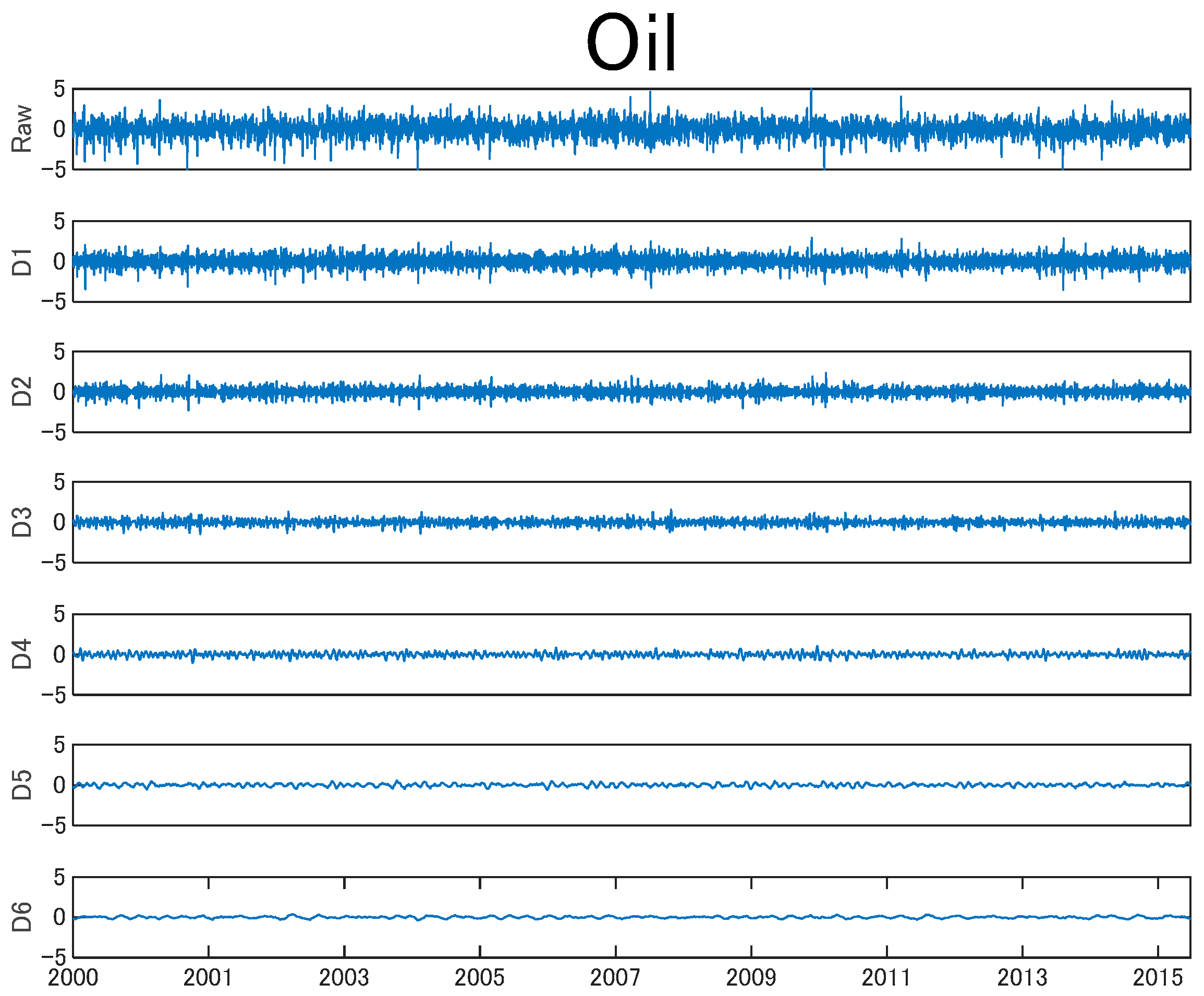
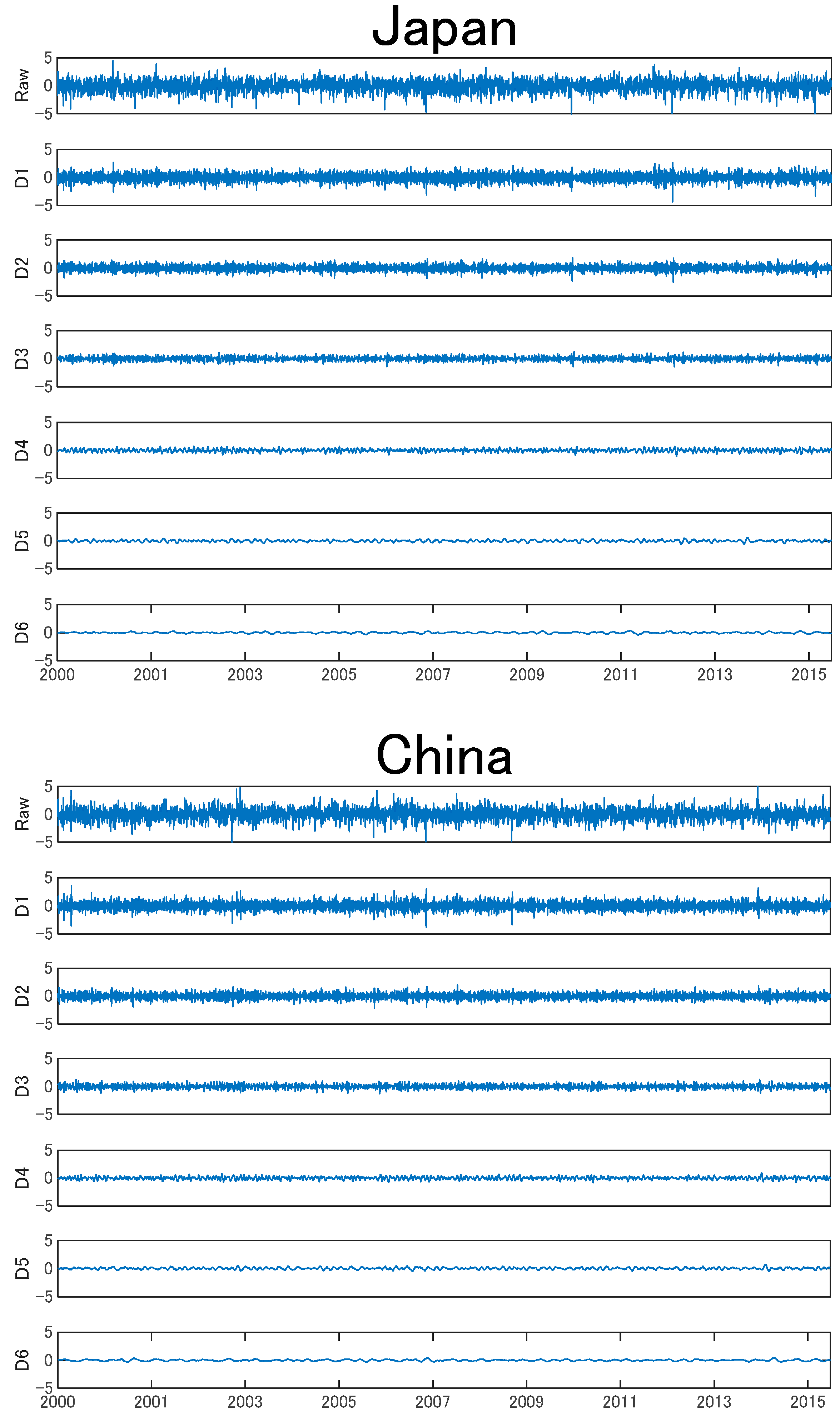
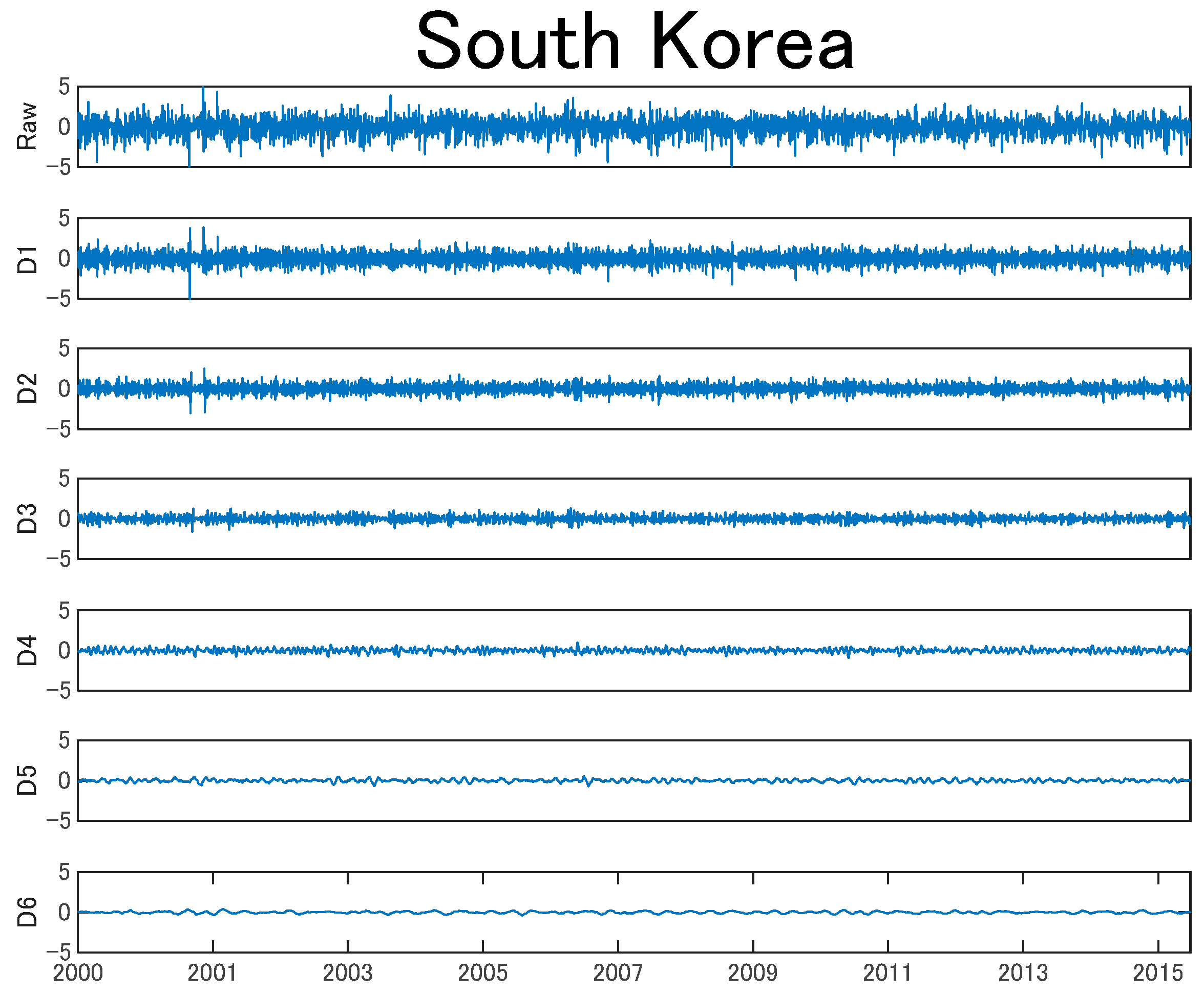
2.2. Maximal Overlap Discrete Wavelet Transform (MODWT)

Next, we use wavelet analysis to decompose the estimated standardized shocks ${\widehat{z}}_{i,t}$ into different time scales in order to capture the dynamics of the series across different time scales. Specifically, we apply the maximal overlap discrete wavelet transform (MODWT) which can overcome the dyadic length sample size (i.e., a sample size divisible by $2^J$) restriction of discrete wavelet transform (DWT). In Section 2.2.1 and Section 2.2.2, we seek to provide a brief review of a few DWT and MODWT techniques. Many more details can be found in the references [21,22,23].

2.2.1. Discrete Wavelet Transform (DWT) and DWT-Based Multi-Resolution Analysis

Here, we provide a brief discussion on the DWT and its multi-resolution analysis. We denote the wavelet (high-frequency) filter by $h_l, l=0,\dots ,L-1$ and the scaling (low-frequency) filter by $g_l, l=0,\dots ,L-1$ for discrete compactly supported filters of the Daubechies class [24]. By definition, the wavelet filter satisfies

$${{\displaystyle \sum }}_{l=0}^{L-1}{h}_l=0, {{\displaystyle \sum }}_{l=0}^{L-1}{h}_l^2=1, {{\displaystyle \sum }}_{l=0}^{L-1}{h}_l{h}_{l+2n}=0$$

(6)

for all nonzero integers n so that the wavelet filter sums to 0, has unit energy, and is orthogonal to its even shifts. The scaling filter $g_l$ is also required to satisfy the last two conditions of Equation (6).

Besides, the wavelet and the scaling filter have the quadrature mirror filter relationship satisfying

$$h_l={\left(-1\right)}^l{g}_{L-l-1} or g_l={\left(-1\right)}^{l+1}{h}_{L-l-1}, for l=0,\dots ,L-1$$

(7)

Consider $X_t, t=0,\dots ,N-1$ a column vector of N observations of a real-valued time series. We assume that the sample size N is an integer multiple of $2^J$, where J is a positive integer. The jth level wavelet and scaling coefficients of DWT is given by

$$W_{j,t}={{\displaystyle \sum }}_{l=0}^{L-1}{h}_l{V}_{j-1,\left(2t+1-l\right)modN/2^{j-1}},$$

(8)

$$V_{j,t}={{\displaystyle \sum }}_{l=0}^{L-1}{g}_l{V}_{j-1,\left(2t+1-l\right)modN/2^{j-1}},$$

(9)

where the length of $V_{j-1,t}$ is $\frac{\mathrm{N}}{2^{j-1}}$ and we start the pyramid algorithm from $X_t=V_{0,t}$ with $j=1$. After repeating the algorithm with $j=2, 3, \dots , J$, we obtain all the vectors of wavelet coefficients $W_1,W_2, \dots , W_J$ and a single vector of scaling coefficients V_J (The other vectors of scaling coefficients $V_1,V_2, \dots , V_{J-1}$ can be regarded as intermediate computations.).

Thus, we can reconstruct the jth level time series namely wavelet detail $D_{j,t}$ and wavelet smooth $S_{j,t}$ by using the j + 1th level wavelet and scaling coefficients as follows:

$$D_{j, t}={{\displaystyle \sum }}_{l=0}^{L-1}{h}_l{W}_{j+1, \left(t+l\right)modN/2^j}^o+{{\displaystyle \sum }}_{l=0}^{L-1}{g}_l{V}_{j+1, \left(t+l\right)modN/2^j}^o, t=0,\dots ,\frac{N}{2^j}-1,$$

(10)

where $W_{j,t}^o=\{\begin{array}{c}0, t=0, 2,\dots ,\frac{N}{2^j}-2\\ W_{j,\left(t-1\right)/2}, t=1,3,\dots ,\frac{N}{2^j}-1\end{array}$ and $V_{j,t}^o=\{\begin{array}{c}0, t=0, 2,\dots ,\frac{N}{2^j}-2\\ V_{j,\left(t-1\right)/2}, t=1,3,\dots ,\frac{N}{2^j}-1\end{array}$.

$$S_{j,t}=S_{j-1,t}-D_{j, t}$$

(11)

Thus, we can represent the multi-resolution representation of the original time series by

$$Z_t={{\displaystyle \sum }}_{j=1}^J{D}_{j,t}+S_{J,t},$$

(12)

where Z_t represents the vector of the estimated standardized residuals; and $S_{J,t}$ and $D_{j,t}$ are the Jth order wavelet smooth and the jth order detail, respectively. The wavelet smooth can provide the approximated trend, while the wavelet detail can capture the local variance over the different time scales $2^j$ days.

2.2.2. MODWT and MODWT-Based Multi-Resolution Analysis

Due to some limitations of the DWT, we employ here the MODWT (introduced by [25]). MODWT can overcome the dyadic length sample size requirements of DWT and both the MODWT wavelet and scaling coefficients, and multiresolution analysis are undecimated or shift-invariant [26,27,28].

The wavelet and scaling filters of MODWT ${\tilde{h}}_l$ and ${\tilde{g}}_l$ are rescaled as ${\tilde{h}}_l={\tilde{h}}_l/\sqrt{2}$, and ${\tilde{g}}_l={\tilde{g}}_l/\sqrt{2}$. Thus, we compute the MODWT wavelet and scaling coefficients for levels $j=1, 2, \dots , J$ using circular linear filtering as follows:

$${\tilde{W}}_{j,t}={{\displaystyle \sum }}_{l=0}^{L-1}{\tilde{h}}_l{\tilde{V}}_{j-1, \left(t-2^{j-1}l\right)modN},t=0,\dots , N-1,$$

(13)

$${\tilde{V}}_{j,t}={{\displaystyle \sum }}_{l=0}^{L-1}{\tilde{g}}_l{\tilde{V}}_{j-1, \left(t-2^{j-1}l\right)modN},t=0,\dots , N-1.$$

(14)

Thus, we can reconstruct the MODWT wavelet detail ${\tilde{D}}_{j,t}$ and wavelet smooth ${\tilde{S}}_{j,t}$ as follows:

$${\tilde{D}}_{j, t}={{\displaystyle \sum }}_{l=0}^{L-1}{\tilde{h}}_l{\tilde{W}}_{j+1, \left(t+2^{j}l\right)modN}+{{\displaystyle \sum }}_{l=0}^{L-1}{\tilde{g}}_l{\tilde{V}}_{j+1, \left(t+2^{j}l\right)modN}, t=0,\dots ,N-1,$$

(15)

$${\tilde{S}}_{j,t}={\tilde{S}}_{j-1,t}-{\tilde{D}}_{j, t}.$$

(16)

Then, equation

$$Z_t={\displaystyle \sum }_{j=1}^J{\tilde{D}}_{j,t}+{\tilde{S}}_{J,t}$$

(17)

constitutes an MODWT multi-resolution analysis analogous to Equation (12).

Due to the limitation of the DWT that restricts the sample size to an integer multiple of 2, the MODWT is used in this study. The MODWT can provide all the functions of DWT and is well defined for any sample size. The wavelet and scaling coefficients and multiresolution analysis of MODWT are shift-invariant, implying that it does not change the location of events in time and the pattern of wavelet transform coefficients [21,22,23]. Specifically, [21] documented and proved that the variance of the coefficients of the MODWT can perfectly capture the variance of the original time series. Recently, some studies applied MODWT to analyze or predict the time series in the financial markets. For example, [27] investigated the impact of oil shocks and stock crashes on correlations between oil and stock markets by using MODWT to avoid the lack of translation-invariance of DWT. [29] examines the spillovers in time and frequency from global stock market and oil prices toward African stock markets. They also select the MODWT to obtain the stock and oil returns at different time scales since the MODWT allows to have the data in time series on each scale and to analyze them more easily (unlike the CWT that converts data into a two-dimensional field).

Thus, in our empirical analysis, we employ MODWT to decompose the daily data and choose $J=6$ to measure the local variance over 2 days, 4 days, 8 days, 16 days, 32 days, and 64 days, respectively.

2.3. Copula Functions

Then, we model the dependence structure between two crude oil and stocks by using the conditional copula functions, that is, the conditional joint distribution of the standardized shocks. [30] extended the theorem of [31] to the conditional copula function, which states that conditional joint distribution can be decomposed into different conditional marginal distributions and a conditional copula function.

Consider the bivariate stochastic process $Z_t={\left(z_{1t}, z_{2t}\right)}^{\prime }$ with a conditional joint distribution F, as well as conditional marginal distributions $F_1$ and $F_2$. Thus,

$$F \left(Z_t|{ℱ}_{t-1}\right)= C \left(F_1\left(z_{1t}|{ℱ}_{t-1}\right), F_2\left(z_{2t}|{ℱ}_{t-1}\right)|{ℱ}_{t-1}\right),$$

(18)

where $C$ is the conditional copula of $Z_t$ and ${ℱ}_{t-1}$ is the information set.

We consider the copula functions as follows:

$$U_{it}|{ℱ}_{t-1}=F_i\left(z_{i,t}\right), for i=1, 2,$$

(19)

$$U_t\left|{ℱ}_{t-1}={\left\{u_{1t}, u_{2t}\right\}}^{\prime }\right|{ℱ}_{t-1}~C\left(\kappa \right),$$

(20)

where $\kappa$ is assumed as the parameter of any kind of copula functions.

We take into account possible time variations in the copula function by considering the time-varying dependence parameters according to an evolution equation that assumes a dependence parameter evolved according to an ARMA (1, 10) process-type process (see [30]):

$${\kappa }_t=\Delta (\omega +\beta {\kappa }_{t-1}+\alpha \frac{1}{10}{{\displaystyle \sum }}_{j=1}^{10}\left|u_{1,t-j}-u_{2,t-j}\right|),$$

(21)

where $\Delta \left(x\right)$ is a logistic transformation, parameter $\omega$ is the constant term, $\beta$ is the autoregressive term, and $\alpha$ is the transformed term.

Copula functions can not only measure the dependence between two variables, but they can also provide information on tail dependence by measuring their extreme upward or downward probability. The conditional upper tail dependence (${\tau }^U$) and lower tail dependence (${\tau }^L$) are defined as follows:

$${\tau }^U=li{m}_{u\to 1}\mathrm{Pr}\left[z_2\ge F_2^{-1}\left(u\right)|z_1\ge F_1^{-1}\left(u\right),{ℱ}_{t-1}\right]=li{m}_{u\to 1}\frac{[1-2u+C(u,u|{ℱ}_{t-1})]}{1-u},$$

(22)

$${\tau }^L=li{m}_{u\to 0}\mathrm{Pr}\left[z_2\le F_2^{-1}\left(u\right)|z_1\le F_1^{-1}\left(u\right),{ℱ}_{t-1}\right]=li{m}_{u\to 0}\frac{C(u,u|{ℱ}_{t-1})}{u},$$

(23)

where ${\tau }^U,{\tau }^L\in \left[0, 1\right]$. If ${\tau }^U=0$, the probability of an extremely large value for variable $z_1$ together with an extremely large value for another variable $z_2$ is zero, which means that they are asymptotically independent in the conditional upper tail dependence. If ${\tau }^U\in \left(0, 1\right]$, the variable $z_1$ and $z_2$ are asymptotically upper tail dependent. The conditional lower tail dependence can be described similarly. If ${\tau }^L=0$, the two variables have conditional lower tail independence, while if ${\tau }^L\in \left(0, 1\right]$, then they have conditional lower tail dependence.

Here, we employ normal, Student’s t, rotated Gumbel, Clayton, and symmetrized Joe–Clayton (SJC) copula, to analyze the symmetric and asymmetric dependence and tail dependence structures. Appendix A describes these five copula functions including both constant copula function (as a benchmark) and dynamic copula.

2.4. Estimation Method

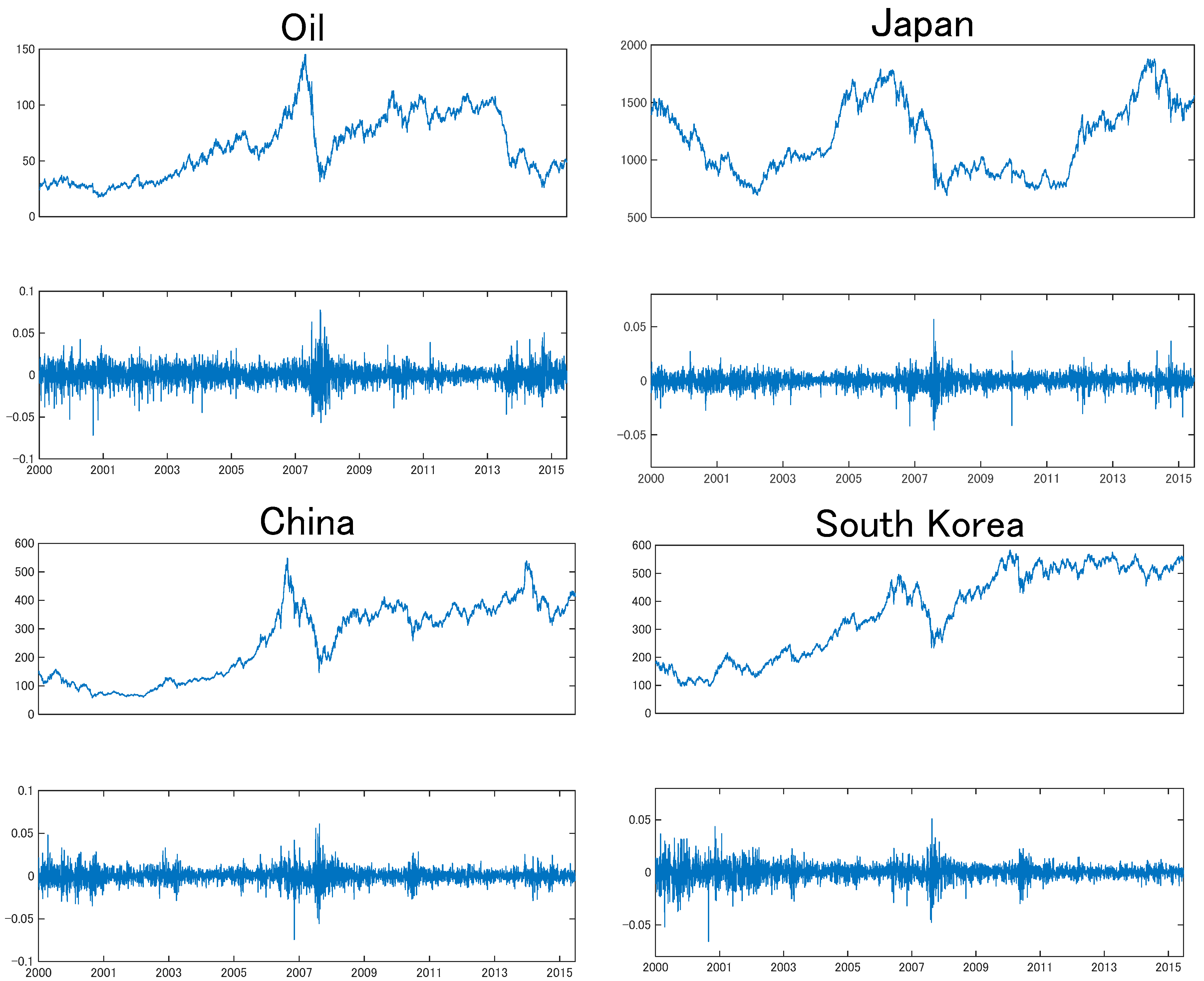
We first estimate the marginal models by using the maximum likelihood estimation (MLE). The log-likelihood function is given by

$${{\displaystyle \sum }}_{t}log{f}_{it}\left(z_{it}; \varphi , \alpha \right)={{\displaystyle \sum }}_{t}log{f}_{1t}\left(z_{1t}; \varphi , \alpha \right)+{{\displaystyle \sum }}_{t}log{f}_{2t}\left(z_{2t}; \varphi , \alpha \right), i=1,2,$$

(24)

where ${\left({\varphi }^{\prime }, {\alpha }^{\prime }\right)}^{\prime }$ are the parameters of the marginal models.

Second, we use the wavelet method to decompose the standardized shocks obtained from marginal models into time series across different timescales.

Finally, we estimate the copula functions scale by scale using MLE. The log-likelihood function is given by

$$log{ℒ}_s\left({\kappa }_s\right)={\displaystyle \sum }_t\log c_s\left(F_{1st}\left(z_{1t};\widehat{\varphi }, \widehat{\alpha } \right),F_{2st}\left(z_{2t};\widehat{\varphi }, \widehat{\alpha } \right);{\kappa }_s\right)$$

(25)

3. Data

Our data consist of daily returns of crude oil and East Asian stock market indexes. West Texas Intermediate (WTI) Cushing Crude Oil Spot Price Index is selected to represent for oil prices. For East Asian stock markets, three representative East Asian countries are selected—Japan, China, and South Korea. All stock indexes are derived from the Morgan Stanley Capital International (MSCI) indexes. Our sample includes 4120 daily observations from 4 January 2000 to 28 October 2016.

Table 1. Descriptive statistics for crude oil and East Asian stock markets.

	Mean	Std.dev.	Skewness	Kurtosis	Jarque-Bera
Oil	01	0.0109	−0.0434	7.0412	2804.1 ***
Japan	00	0.0063	−0.3540	9.2208	6727.7 ***
China	01	0.0081	−0.1059	9.5531	7377.8 ***
South Korea	01	0.0074	−0.3795	9.3222	6958.8 ***

Notes: *** denote the rejection of the null hypotheses of normality at the 1% significance level.

presents the descriptive statistics. Clearly, all returns distributions are against normal as measured by the skewed distribution and excess kurtosis.

Figure 1 plots the price and return series in top and bottom panel, respectively. The prices are represented in US dollars. Oil price is considerably increased from 2006–2007 covering the periods of OPEC cuts and decreased during the global financial crisis. We can clearly observe that East Asian stock prices have also decreased since the 2008 global financial collapse. The volatility of oil and stock returns increased during the 2008 global financial crisis.

4. Empirical Results

In this section, we present the empirical results of the relationship between crude oil and East Asian stock markets. Our application was firstly based on an AR-GJR-GARCH process for marginal distributions. Marginal models and lags were appropriately selected according to the information criteria. These estimates are presented in

Table 2. Estimates of marginal distribution from AR (1)-GJR-GARCH (1, 1, 1) with skewed-t distributions.

	Crude Oil	Japan	China	South Korea
$\mu$	0	0	0	0
	(0)	(0)	(0)	(0)
${\varphi }_1$	−0.041	0.032	0.043	−0.004
	(0.016)	(0.016)	(0.015)	(0.015)
$\mathsf{\omega }$	0	0	0	0
	(0)	(0)	(0)	(0)
$\alpha$	0.023	0.021	0.029	0.014
	(0.004)	(0.009)	(0.003)	(0.004)
$\beta$	0.953	0.890	0.922	0.943
	(0.007)	(0.015)	(0.008)	(0.004)
$\mathsf{\gamma }$	0.041	0.124	0.076	0.075
	(0.009)	(0.022)	(0.009)	(0.010)
$\lambda$	0.924	0.929	0.979	0.931
	(0.020)	(0.020)	(0.020)	(0.018)
$\eta$	8.256	8.651	6.816	6.521
	(0.491)	(1.196)	(0.643)	(0.642)
$Q$(30)	0.791	0.973	0.190	0.682
$Q^2$(30)	0.138	0.768	0.184	0.545

Notes: Standard errors are in parentheses. The optimal AR and GARCH lags are selected according to information criteria.

. Clearly, GARCH and distributional parameters were all significant. The Q-test showed no autocorrelation in (squared) standardized residuals, indicating that the marginal distributions awere properly specified.

Then, the standardized shocks for each variable were decomposed using MODWT analysis up to six levels, D1 to D6, covering the short-term, midterm, and long-term horizons. D1 (two days) and D2 (four days) represent the fluctuation of prices in the short-term horizon. D3 (eight days) and D4 (16 days) represent the fluctuation occurring in the midterm horizon. D5 (32 days) and D6 (64 days) represent for the long term horizon in this study.

Figure 2 shows the wavelet decompositions of crude oil and East Asian stock markets from D1 to D6, ranging from the highest to the lowest frequency. Obviously, in all markets, the level of fluctuations decreased as time scales increased, suggesting that market price was much noisier in the short term than in the mid- and long-term.

Next, we capture the joint behavior of stock and crude oil across the multiple time scales by using the conditional copula functions. Five copula functions are considered to analyze the constant and dynamic interdependence of pairs and their tail dependence, including normal, rotated Gumbel, Clayton, Student’s t, and SJC copulas. These copulas could capture different types of interdependence, with regard of asymmetry and tail dependence. The copula density functions are given in the Appendix A.

The constant copula estimates are reported in

Table 3. Constant copula estimates of crude oil with East Asian stock market across multiple timescales.

	Japan							China							South Korea
	Raw	D1	D2	D3	D4	D5	D6	Raw	D1	D2	D3	D4	D5	D6	Raw	D1	D2	D3	D4	D5	D6
Normal
$\mathsf{\rho }$	0.069	0.008	0.111	0.142	0.085	0.176	0.234	0.112	0.039	0.155	0.175	0.212	0.283	0.277	0.115	0.057	0.148	0.185	0.159	0.170	0.285
	(0.015)	(0.020)	(0.019)	(0.019)	(0.025)	(0.030)	(0.019)	(0.015)	(0.019)	(0.019)	(0.019)	(0.025)	(0.028)	(0.019)	(0.015)	(0.019)	(0.019)	(0.019)	(0.026)	(0.030)	(0.018)
log$ℒ$	9.807	0.129	25.350	41.659	14.810	64.622	116.356	25.884	3.160	50.066	63.891	95.053	171.456	164.292	27.293	6.608	45.477	71.346	52.904	60.130	174.298
GOF	0.640	0.920	0.890	0.130	0.350	0.540	0.100	0.340	0.540	0.420	0.140	0.290	0.680	0	0.670	0.940	0.710	0.820	0.110	0.070	0.280
Clayton
$\mathsf{\kappa }$	0.067	0.015	0.185	0.252	0.243	1.118	2.413	0.130	0.076	0.257	0.338	0.576	1.415	2.359	0.120	0.100	0.234	0.344	0.440	1.108	2.502
	(0.017)	(0.021)	(0.027)	(0.028)	(0.033)	(0.044)	(0.056)	(0.019)	(0.025)	(0.027)	(0.028)	(0.033)	(0.045)	(0.056)	(0.019)	(0.026)	(0.027)	(0.028)	(0.033)	(0.044)	(0.057)
${\mathsf{\tau }}^{\mathrm{L}}$	0	0	0.023	0.064	0.057	0.538	0.750	0.005	0	0.067	0.128	0.294	0.613	0.745	0.003	0.001	0.052	0.133	0.207	0.535	0.758
log$ℒ$	8.871	0.195	26.195	42.014	25.222	266.924	818.850	29.088	4.892	48.171	76.385	142.574	438.961	806.460	24.742	8.244	40.391	77.834	83.290	260.970	886.425
GOF	0.480	0.210	0.040	0	0.010	0	0	0.640	0	0	0.010	0	0	0	0.450	0.630	0.050	0	0.020	0	0
Rotated Gumbel
$\mathsf{\kappa }$	1.034	1.018	1.099	1.139	1.132	1.673	2.473	1.071	1.047	1.139	1.177	1.296	1.862	2.471	1.066	1.061	1.130	1.187	1.229	1.668	2.539
	(0.009)	(0.012)	(0.013)	(0.014)	(0.016)	(0.027)	(0.035)	(0.011)	(0.013)	(0.014)	(0.015)	(0.019)	(0.028)	(0.035)	(0.011)	(0.013)	(0.014)	(0.015)	(0.018)	(0.027)	(0.036)
${\mathsf{\tau }}^{\mathrm{L}}$	0.045	0.025	0.121	0.162	0.155	0.487	0.677	0.090	0.062	0.162	0.198	0.293	0.549	0.676	0.085	0.079	0.154	0.207	0.242	0.485	0.686
log$ℒ$	8.446	1.338	31.604	54.808	37.146	325.876	973.632	32.569	7.968	59.365	87.819	156.087	517.525	981.967	27.484	13.357	51.723	95.710	97.195	319.391	1.053E03
GOF	0.250	0.150	0.050	0	0.050	0	0	0.840	0.380	0	0.150	0	0	0	0.240	0.690	0.030	0	0.080	0	0
Student’s t
$\mathsf{\rho }$	0.069	0.006	0.122	0.157	0.112	0.381	0.614	0.112	0.048	0.174	0.199	0.256	0.518	0.639	0.115	0.068	0.170	0.207	0.201	0.372	0.653
	(0.016)	(0.019)	(0.019)	(0.018)	(0.020)	(0.029)	(0.052)	(0.016)	(0.019)	(0.018)	(0.018)	(0.020)	(0.027)	(0.096)	(0.016)	(0.019)	(0.018)	(0.018)	(0.020)	(0.030)	(0.066)
${\mathsf{\eta }}^{-1}$	0	0.166	0.206	0.363	0.488	0.667	0.909	0.030	0.196	0.217	0.350	0.501	0.667	0.909	0.026	0.188	0.241	0.407	0.467	0.667	0.909
	(0)	(0.035)	(0.036)	(0.032)	(0.032)	(0.047)	(0.149)	(0.016)	(0.033)	(0.035)	(0.032)	(0.033)	(0.062)	(0.315)	(0.029)	(0.034)	(0.034)	(0.031)	(0.033)	(0.047)	(0.223)
$\mathsf{\tau }$	0.005	0.034	0.077	0.178	0.215	0.381	0.549	0	0.056	0.097	0.186	0.275	0.450	0.563	0	0.055	0.111	0.217	0.240	0.377	0.572
log$ℒ$	9.806	8.438	37.583	86.714	101.237	522.136	1.107E03	27.916	17.577	66.303	109.867	204.256	687.731	1.143E03	28.597	18.521	65.776	140.545	143.103	524.385	1.180E03
GOF	0.680	0.350	0.790	0.870	0.760	0.100	0.150	0.170	0.550	0.760	0.230	0.330	0.720	0	0.770	0.840	0.710	0.900	0.360	0.110	0.390
SJC
${\mathsf{\tau }}^{\mathrm{U}}$	0	0	0.049	0.113	0.080	0.507	0.718	0	0	0.098	0.078	0.180	0.578	0.740	0.001	0	0.121	0.130	0.143	0.515	0.737
	(0)	(0)	(0.029)	(0.030)	(0.037)	(0.016)	(0.008)	(0.002)	(0)	(0.029)	(0.032)	(0.033)	(0.013)	(0.007)	(0.003)	(0)	(0.029)	(0.030)	(0.034)	(0.016)	(0.007)
${\mathsf{\tau }}^{\mathrm{L}}$	0.002	0	0.026	0.041	0.080	0.477	0.703	0.035	0.011	0.059	0.142	0.280	0.549	0.686	0.020	0.024	0.023	0.119	0.208	0.473	0.709
	(0.003)	(0)	(0.026)	(0.028)	(0.037)	(0.018)	(0.010)	(0.070)	(0.011)	(0.028)	(0.030)	(0.025)	(0.015)	(0.010)	(0.012)	(0.004)	(0.026)	(0.031)	(0.029)	(0.019)	(0.009)
log$ℒ$	9.817	0.196	34.121	61.196	37.787	433.488	1.163E03	31.686	5.736	66.539	90.553	171.933	650.844	1.203E03	29.012	10.434	62.106	102.417	106.582	435.570	1.251E03
GOF	0.970	0.920	0.960	1	1	1	1	1	0.950	0.990	1	1	1	0.980	0.920	0.940	0.950	1	0.910	1	1

Notes: $\mathsf{\rho }$ is the dependence parameter, $\mathsf{\tau }$ denotes the tail dependence parameter, and ${\mathsf{\tau }}^{\mathrm{U}},{\mathsf{\tau }}^{\mathrm{L}}$ are upper and lower tail dependence parameters respectively. Bootstrapped standard errors are reported in parentheses. GOF refers to p-values of the Cramer-von Mises goodness-of-fit tests. Raw represents the raw return series.

. Generally, the oil-stock dependencies increase and become more significant as the time scales increase. According to log-likelihood and goodness-of-fit test, obviously, SJC copula describes the oil-stock dependencies most appropriately and accurately, suggesting that crude oil and stock returns are asymmetrically upper and lower tail dependent. The estimates of SJC copulas show that, except the very short-term (D1), crude oil and East Asian stock markets are significantly tail dependent. These results indicate that crude oil and stock markets response to identical macroeconomic shocks, however, may not simultaneously.

Since the constant SJC copula describes the oil-stock dependencies best, we use the time-varying SJC copula function to investigate the dynamic dependence structures. These estimates are summarized in

Table 4. Time-varying symmetrized Joe–Clayton (SJC) copula estimates of crude oil with Japanese stock market across different timescales.

	Japan							China							South Korea
	Raw	D1	D2	D3	D4	D5	D6	Raw	D1	D2	D3	D4	D5	D6	Raw	D1	D2	D3	D4	D5	D6
${\omega }^U$	−12.81	−13.47	1.57	4.69	5.91	3.64	7.78	−11.74	−20.69	1.29	4.30	5.88	7.96	2.44	−9.87	−14.31	1.88	4.44	6.22	7.24	2.20
	(2.35)	(0.57)	(0.49)	(0.48)	(0.39)	(0.10)	(0.14)	(2.55)	(0.40)	(0.43)	(0.37)	(0.37)	(0.18)	(0.34)	(8.59)	(0.63)	(0.49)	(0.30)	(0.27)	(0.07)	(0)
${\alpha }^U$	0.03	0	−16.29	−23.51	−25.15	−15.96	−21.41	0.08	0	−12.25	−21.78	−25.48	−28.01	−11.45	−3.38	0.01	−14.12	−20.81	−26.98	−24.57	−14.06
	(0.29)	(0)	(2.97)	(2.50)	(1.64)	(0.24)	(0.36)	(0.72)	(0)	(1.97)	(1.81)	(2.16)	(1.80)	(1.35)	(10.93)	(0)	(2.46)	(1.63)	(2.20)	(0.86)	(0)
${\beta }^U$	0	0	0.32	−3.47	−3.97	0.98	−4.61	0	0	0.52	−3.53	−4.06	−4.67	0.68	−0.01	0	0.93	−3.51	−3.99	−4.37	1.07
	(0)	(0)	(0.80)	(0.13)	(0.12)	(0.01)	(0.05)	(0.30)	(0.01)	(0.45)	(0.18)	(0.11)	(0.07)	(0.24)	(0)	(0)	(0.44)	(0.14)	(0.12)	(0.07)	(0)
${\omega }^L$	−10.01	−14.08	2.09	4.79	6.89	6.92	8.10	0.23	3.45	1.32	5.11	6.62	6.93	2.30	2.45	2.54	2.40	4.19	6.29	7.20	2.03
	(7.62)	(0.51)	(0.58)	(0.38)	(0.28)	(0.12)	(0.04)	(0.87)	(0.80)	(0.49)	(0.28)	(0.27)	(0.23)	(0.47)	(1.06)	(0.66)	(0.65)	(0.27)	(0.26)	(0.23)	(0)
${\alpha }^L$	−2.27	0	−18.63	−22.96	−29.38	−24.34	−22.88	−12.78	−23.62	−13.33	−21.91	−23.85	−23.88	−12.16	−20.54	−17.67	−19.17	−19.95	−24.93	−27.22	−14.07
	(2.64)	(0)	(3.15)	(1.86)	(2.12)	(0.26)	(0.25)	(3.62)	(3.91)	(2.21)	(1.51)	(1.47)	(2.02)	(1.71)	(5.34)	(2.77)	(3.64)	(1.51)	(1.88)	(1.05)	(0)
${\beta }^L$	0.01	0	0.24	−3.37	−4.05	−4.13	−4.97	1.66	−4.61	0.71	−3.51	−4.09	−4.33	0.82	−11.62	−5.95	−1.81	−3.42	−4.04	−4.31	1.43
	(0.01)	(0)	(0.72)	(0.17)	(0.08)	(0.09)	(0.03)	(1.41)	(1.36)	(0.85)	(0.14)	(0.11)	(0.06)	(0.34)	(3.75)	(2.31)	(1.30)	(0.14)	(0.10)	(0.17)	(0)
log$ℒ$	9.02	−2.840	64.32	227.79	469.93	985.88	1939	35.97	12.72	101.49	300.78	586.14	1252	2083	33.03	21.60	105.82	289.50	478.24	1011	1966

Notes: Bootstrapped standard errors are reported in parentheses. log$ℒ$ is the value of log-likelihood.

. Clearly, most estimates are highly significant. According to the log-likelihood, we find that the dynamic copula offers a better fit compared to the constant copulas for in most cases, providing strong evidence that the relationship between crude oil and East Asian stock markets is time-varying at all investment horizons.

Figure 3 shows the time-varying tail dependencies by dynamic SJC copula for each of the oil-stock pair. These figures provide an intuitive impression into the time-varying tail dependence. Looking at these figures, we first find that tail dependencies varied significantly over time and differed in terms of the time horizons. The magnitude of these tail dependencies increasedas the time scales increased. Specifically, we found very weak tail dependence in the short term, which showed the absence of co-movements between crude oil and East Asian stock markets during very short time. However, the tail dependence increased as the time scales increased and differed in bear and bull markets. These results suggest that crude oil market was more likely to be tail dependent with East Asian stock markets in the mid- and long-term than in the short term. In other words, oil market would, but not simultaneously, react to the same extreme events with East Asian stock markets. The possible reasons are (1) the accurate assessment of the market impact of extreme shocks, costing investors some time, and (2) the gradual information diffusion hypothesis by [32]. These results are important in terms of hedging strategies and portfolio risk management.

In sum, according to Figure 2 and Figure 3, we can conclude that short-term signals are more volatile, and the relationship between short-term signals is weak and stable. While long-term signals are less volatile, but their relationship is strong and instable. That is because, the short-term signals are noisy, and there is no relationship between noise trading in crude oil and stock markets. While in the long term, both markets are more likely to suffer from the same macroeconomic shocks.

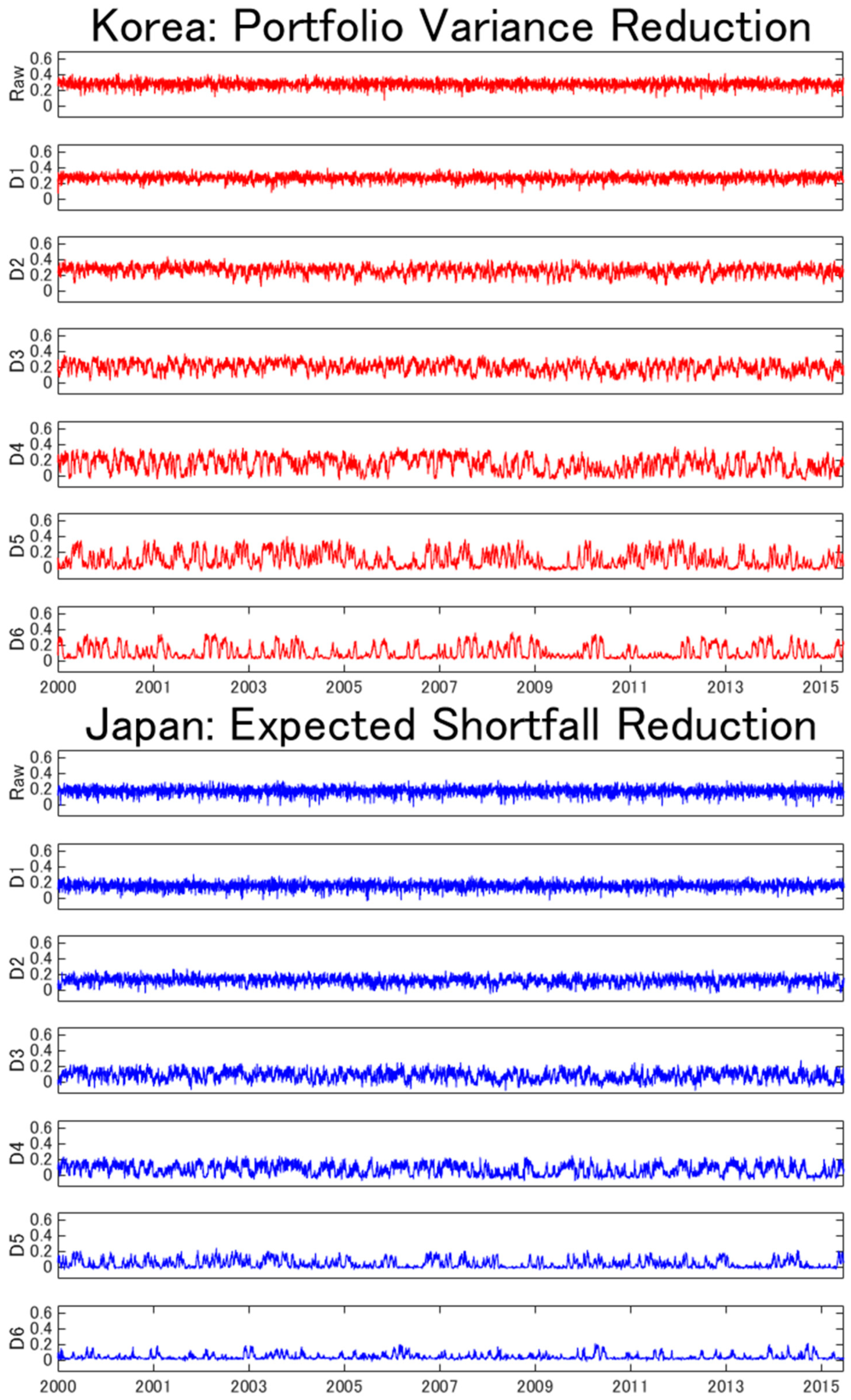
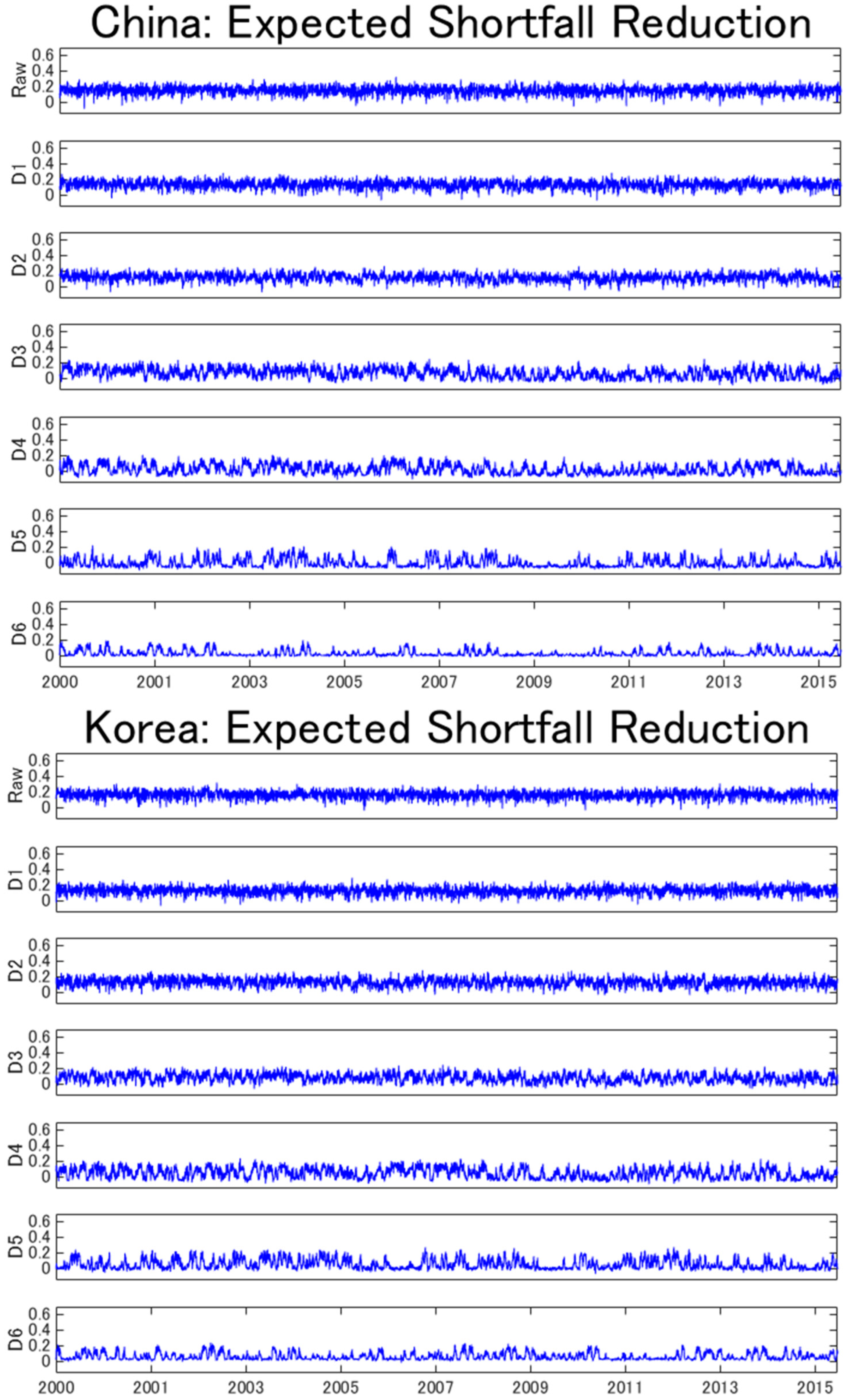
5. Risk Management Analysis

In this section, we investigate risk management implications of oil-stock dependence at multiple time scales. Generally, an asset is defined as a hedge or a safe haven if it is uncorrelated or negatively correlated with another asset or portfolio on average or in times of extreme market movements. Therefore, we examine hedging effectiveness and downside risk hedging performance by comparing the portfolio variance (PV) and expected shortfall (ES). Here, we consider two portfolios, the stock only portfolio and the oil-stock portfolio. For oil-stock portfolio, we randomly generate 100 weights from 0 to 1, and investigate the average performance of these portfolios. We simulate 1000 observations from our model for each portfolio. We choose the best-fit copula—the time-varying SJC copula, and then form the portfolio returns using the wavelet counterparts:

$$r_{s,t}^{portfolio}=w^{oil}{r}_{s,t}^{oil}+\left(1-w^{oil}\right)r_{s,t}^{stock}$$

(26)

where s represents the time scales, w is the weight. We consider percentage portfolio variance (PV) reduction of oil-stock portfolio with respect to stock only portfolio at multiple time scales in terms of the risk reduction (RR) effectiveness ratio as follows:

$$R{R}_{s,t}^{PV}=1-\frac{P{V}_{s,t}^{Portfolio}}{P{V}_{s,t}^{stock}},$$

(27)

A higher value of $R{R}_{s,t}^{PV}$ means greater variance reduction, implying that oil can provide higher hedging benefits against East Asian stock markets.

Table 5. Portfolio variance and expected shortfall reduction effectiveness of oil-stock portfolios at multiple time scales.

	Raw	D1	D2	D3	D4	D5	D6
Panel A. Portfolio variance
Japan	0.295	0.296	0.262	0.222	0.200	0.104	0.063
	(0.048)	(0.042)	(0.055)	(0.081)	(0.100)	(0.089)	(0.065)
China	0.295	0.296	0.265	0.206	0.120	0.088	0.121
	(0.047)	(0.044)	(0.055)	(0.080)	(0.093)	(0.098)	(0.072)
South Korea	0.280	0.272	0.265	0.203	0.152	0.106	0.112
	(0.048)	(0.045)	(0.060)	(0.071)	(0.100)	(0.102)	(0.085)
Panel B. Expected shortfall
Japan	0.176	0.159	0.125	0.084	0.075	0.044	0.043
	(0.053)	(0.049)	(0.052)	(0.065)	(0.071)	(0.055)	(0.036)
China	0.152	0.135	0.119	0.069	0.025	−0.002	0.031
	(0.052)	(0.052)	(0.050)	(0.063)	(0.062)	(0.059)	(0.039)
South Korea	0.164	0.128	0.130	0.081	0.048	0.056	0.063
	(0.050)	(0.051)	(0.054)	(0.055)	(0.067)	(0.065)	(0.047)

Notes: Standard errors are reported in parentheses.

panel A reports the PV reduction performance. Overall, all PV reduction values are positive, indicating that oil is useful in hedging the risk of East Asian stock portfolio at different investment horizons. On the other hand, these PV reduction values and their significance decrease as the time scales increase. Specifically, the hedging benefits are significant from D1 to D3, but most of these values are insignificant from D4 to D6. These results suggest a stronger hedging benefits in the short-term than those in the mid- and long-term.

In addition, we examine the usefulness of crude oil in hedging downside risk performance by estimating the expected shortfall (ES) of a portfolio composed of oil and stock. The ES is given by

$$E{S}_{s,t}=E[r_{s,t}^{portfolio}|r_{s,t}^{portfolio}\le Va{R}_{s,t}],$$

(28)

where $Va{R}_{s,t}=F_{s,t}^{-1}\left(q\right)$ represents the value at risk at the $\left(1-q\right)\%$ confidence level of a portfolio and $F(.)$ is the conditional joint distribution. Similarly, we evaluated downside risk gains by evaluating percentage ES reduction of oil-stock portfolio with respect to stock only portfolio at different time scales in terms of the risk reduction (RR) effectiveness ratio as follows:

$$R{R}_{s,t}^{ES}=1-\frac{E{S}_{s,t}^{Portfolio}}{E{S}_{s,t}^{stock}}.$$

(29)

Regarding downside risk, Table 5 panel B presents the results for the ES reduction. Similarly, most of these values are positive, implying that crude oil is useful in hedging the downside risk of East Asian stock market. The ES reduction ratios are bigger and more likely to be significant in the short-term than in the mid- and long-term.

Figure 4 displays dynamic PV and ES reduction effectiveness. These plots offer graphical insights into the nature of the dynamic hedging and downside risk reduction at multiple time scales. Clearly, most values are positive over time and across frequencies, implying that crude oil is useful in reducing the risk and downside risk of East Asian stock markets over the whole sample period. The short-term hedging benefits are stable, while the mid- and long-term PV and ES reduction ratios vary dramatically over time. Moreover, the hedging benefits have been reduced in the long-run.

Overall, these results point to the value of using crude oil as a hedge and safe haven against East Asian stock markets, although the hedging benefits would vary across markets and investment horizons.

6. Conclusions

Crude oil is widely recognized as a strategic commodity. Its price volatility and influence has become crucial for world economic development. Besides, crude oil has become important investment tool for portfolio diversification and risk management. It is important to understand the dependence and tail dependence of oil and stock markets at multiple investment time horizons.

This paper investigates the time-varying dependence and tail dependence between crude oil and East Asian stock markets across multiple time scales. We also assess the risk and downside risk hedging benefits of crude oil to East Asian stock markets. Our results provide strong evidence of time-varying dependence and asymmetric tail dependence between crude oil and stock markets at different time scales. The oil-stock dependence and tail dependence increase as the time-scale increases. Short-term signals are volatile, and their relationship is weak and stable. In contrast, long-term signals are less volatile, but their relationship is strong and instable.

Based on the analysis of the risk reduction of portfolio variance and expected shortfall, we investigate the risk and tail risk hedging performance of crude oil to stock portfolios. We find strong evidence that the hedging effectiveness vary over time and differ in terms of investment horizons. All PV and ES risk reduction values are bigger than zero, suggesting that crude oil is useful in diversifying the East Asian stock portfolio. We also find that hedging benefits decrease as time scales increase, indicating that oil is more useful in hedging the risk in the short-term than in the mid- and long-term. These results are in line with previous results of oil-stock dependence. From the statistical perspective, increasing positive relationship would decrease hedging benefits. From the economic perspective, oil and stock markets are influenced by similar macroeconomic shocks in the long-term. Our results have important implications for heterogeneous investors and market participants.

References

1. Arouri, M.H.; Hammoudeh, S.; Lahiani, A.; Nguyen, D.K. On the Short- and Long-run Efficiency of Energy and Precious Metal Markets. Energy Econ. 2013, 40, 832–844. [Google Scholar] [CrossRef] [Green Version]
2. Daskalaki, C.; Skiadopoulos, G. Should Investors Include Commodities in Their Portfolios After All? New Evidence. J. Bank. Financ. 2011, 35, 2606–2626. [Google Scholar] [CrossRef]
3. Arouri, M.H.; Nguyen, D.K. Oil prices, stock markets and portfolio investment: Evidence from sector analysis in Europe over the last decade. Energy Policy 2010, 38, 4528–4539. [Google Scholar] [CrossRef] [Green Version]
4. Avdulaj, K.; Barunik, J. Are benefits from oil-stocks diversification gone? New evidence from a dynamic copula and high frequency data. Energy Econ. 2015, 51, 31–44. [Google Scholar] [CrossRef] [Green Version]
5. Balcilar, M.; Ozdemir, Z.A. The causal nexus between oil prices and equity market in the U.S.: A regime switching model. Energy Econ. 2013, 39, 271–282. [Google Scholar] [CrossRef]
6. Hayate, G. Linking the gas and oil markets with the stock market: Investigating the U.S. relationship. Energy Econ. 2016, 53, 5–15. [Google Scholar]
7. Huang, S.; Haizhong, A.; Gao, X.; Sun, X. Do oil price asymmetric effects on the stock market persist in multiple time horizons? Appl. Energy 2017, 185, 1799. [Google Scholar] [CrossRef]
8. Sadorsky, P. The macroeconomic determinants of technology stock price volatility. Rev. Financ. Econ. 2003, 12, 191–205. [Google Scholar] [CrossRef]
9. Sadorsky, P. Correlations and volatility spillovers between oil prices and the stock prices of clean energy and technology companies. Energy Econ. 2012, 1, 248–255. [Google Scholar] [CrossRef]
10. Dent, C.M. Paths ahead for East Asia and Asia-Pacific regionalism. Int. Aff. 2013, 89, 963–985. [Google Scholar] [CrossRef]
11. Cai, X.J.; Hamori, S. Business cycle volatility and hot money in emerging east Asian markets. In Financial Linkages, Remittances, and Resource Dependence in East Asia; WSPC: Albemarle, NC, USA, 2015; pp. 59–80. [Google Scholar]
12. Cai, X.J.; Tian, S.; Yuan, N.; Hamori, S. Interdependence between oil and East Asian stock markets: Evidence from wavelet coherence analysis. J. Int. Financ. Mark. Inst. Money 2001, 48, 206–223. [Google Scholar] [CrossRef]
13. Shin, E.; Savage, T. Joint stockpiling and emergency sharing of oil: Arrangements for regional cooperation in East Asia. Energy Policy 2011, 39, 2817–2823. [Google Scholar] [CrossRef]
14. Ciner, C. Energy shocks and financial markets: Nonlinear linkages. Stud. Nonlinear Dyn. Econom. 2017, 5, 1–11. [Google Scholar]
15. Fratzscher, M.; Schneider, D.; Van Robays, I. Oil Prices, Exchange Rates and Asset Prices; ECB Working Paper Series (1689) (July); European Central Bank: Frankfurt, Germany, 2014. [Google Scholar]
16. Bjørnland, H.C. Oil price shocks and stock market booms in an oil exporting country. Scott. J. Political Econ. 2009, 56, 232–254. [Google Scholar] [CrossRef] [Green Version]
17. Jammazi, R.; Reboredo, J.C. Dependence and risk management in oil and stock markets. A wavelet-copula analysis. Energy 2016, 107, 866–888. [Google Scholar] [CrossRef]
18. Jia, X.; An, H.; Fang, W.; Sun, X.; Huang, X. How do correlations of crude oil prices co-move? A grey correlation-based wavelet perspective. Energy Econ. 2015, 49, 588–598. [Google Scholar] [CrossRef]
19. Glosten, L.R.; Jagannathan, R.; Runkle, D.E. On the relation between the expected values and the volatility of the nominal excess return on stocks. J. Financ. 1993, 48, 1779–1801. [Google Scholar] [CrossRef]
20. Hansen, B.E. Autoregressive conditional density estimation. Int. Econ. Rev. 1994, 35, 705–730. [Google Scholar] [CrossRef]
21. Percival, D.B.; Mofjeld, H. Analysis of subtidal coastal sea level fluctuations using wavelets. J. Am. Stat. Assoc. 1997, 92, 868–880. [Google Scholar] [CrossRef]
22. Percival, D.B.; Walden, A.T. Wavelet Methods for Time Series Analysis; Cambridge University Press: Cambridge, UK, 2000. [Google Scholar]
23. Serroukh, A.; Walden, A.T.; Percival, D.B. Statistical properties and uses of the wavelet variance estimator for the scale analysis of time series. J. Am. Stat. Assoc. 2000, 95, 184–196. [Google Scholar] [CrossRef]
24. Daubechies, I. Ten Lectures on Wavelets; SIAM: Philadelphia, PA, USA, 1992. [Google Scholar]
25. Barnes, J.A.; Chi, A.R.; Cutler, L.S.; Healey, D.J.; Leeson, D.B.; Mcgunigal, T.E.; Mullen, J.A.; Smith, W.L.; Sydnor, R.L.; Vessot, R.F.C.; et al. Characterization of frequency stability. IEEE Trans. Instrum. Meas. 1971, 20, 105–120. [Google Scholar] [CrossRef] [Green Version]
26. Liang, J.; Parks, T.W. A translation-invariant wavelet representation algorithm with applications. IEEE Trans. Signal Porcess. 1996, 44, 225–232. [Google Scholar] [CrossRef]
27. Martín-Barragán, B.; Ramos, S.B.; Veiga, H. Correlations between oil and stock markets: A wavelet-based approach. Econ. Model. 2015, 50, 212–227. [Google Scholar] [CrossRef]
28. Shensa, M.J. The discrete wavelet transform: Wedding the àtrous and mallat algorithms. IEEE Trans. Signal Process. 1992, 40, 2464–2482. [Google Scholar] [CrossRef] [Green Version]
29. Gourène, G.A.Z.; Mendy, P.; Ake, G.M.N. Multiple time-scales analysis of global stock markets spillovers effects in African stock markets. Int. Econ. 2019, 157, 82–98. [Google Scholar] [CrossRef]
30. Patton, A.J. Modeling asymmetric exchange rate dependence. Int. Econ. Rev. 2006, 47, 527–556. [Google Scholar] [CrossRef]
31. Sklar, A. Fonctions de Repartition à n Dimensions et Leurs Marges; Publications de l’Institut de Statistique de l’Universite de Paris: Paris, France, 1959; Volume 8, pp. 229–231. [Google Scholar]
32. Hong, H.G.; Stein, J. A unified theory of underreaction, momentum trading and overreaction in asset markets. J. Financ. 1999, 54, 2143–2148. [Google Scholar] [CrossRef] [Green Version]
Figure 1. Time series of prices and returns.
Energies 13 00294 g001
Figure 2. Wavelet decomposition of standardized residuals for crude oil and East Asian stock markets. Raw represents the original time series. D1 (two days) and D2 (four days) represent the short-term fluctuations. D3 (eight days) and D4 (16 days) represent for the mid-term. D5 (32 days) and D6 (64 days) represent for the long term.
Energies 13 00294 g002aEnergies 13 00294 g002bEnergies 13 00294 g002c
Figure 3. Time-varying tail dependence between crude oil and East Asian stock markets from SJC copula estimates.
Energies 13 00294 g003aEnergies 13 00294 g003bEnergies 13 00294 g003cEnergies 13 00294 g003d
Figure 4. Dynamic portfolio variance and expected shortfall reduction effectiveness for oil-stock portfolios at the multiple time scales.
Energies 13 00294 g004aEnergies 13 00294 g004bEnergies 13 00294 g004c