
Evaluation of Deep Learning-Based Non-Intrusive Thermal Load Monitoring
by
 , , , , , and
Kazuki Okazawa
1,*,
Naoya Kaneko
1,
Dafang Zhao
1,
Hiroki Nishikawa
1,
Ittetsu Taniguchi
1,
Francky Catthoor
2,3 and
Takao Onoye
1 1
Graduate School of Information Science and Technology, Osaka University, 1-5 Yamadaoka, Suita 565-0871, Osaka, Japan
2
Interuniversity Microelectronics Centre (IMEC), Kapeldeef 75, 3001 Heverlee, Belgium
3
Department of Electrical Engineering (ESAT), KU Leuven, Kasteelpark Arenberg 10, 3001 Leuven, Belgium
*
Author to whom correspondence should be addressed.
Energies 2024, 17(9), 2012; https://doi.org/10.3390/en17092012
Submission received: 23 March 2024
/
Revised: 18 April 2024
/
Accepted: 19 April 2024
/
Published: 24 April 2024
(This article belongs to the Section G: Energy and Buildings)
Abstract
:Non-Intrusive Load Monitoring (NILM), which provides sufficient load for the energy consumption of an entire building, has become crucial in improving the operation of energy systems. Although NILM can decompose overall energy consumption into individual electrical sub-loads, it struggles to estimate thermal-driven sub-loads such as occupants. Previous studies proposed Non-Intrusive Thermal Load Monitoring (NITLM), which disaggregates the overall thermal load into sub-loads; however, these studies evaluated only a single building. The results change for other buildings due to individual building factors, such as floor area, location, and occupancy patterns; thus, it is necessary to analyze how these factors affect the accuracy of disaggregation for accurate monitoring. In this paper, we conduct a fundamental evaluation of NITLM in various realistic office buildings to accurately disaggregate the overall thermal load into sub-loads, focusing on occupant thermal load. Through experiments, we introduce NITLM with deep learning models and evaluate these models using thermal load datasets. These thermal load datasets are generated by a building energy simulation, and its inputs for the simulation were derived from realistic data like HVAC on/off data. Such fundamental evaluation has not been done before, but insights obtained from the comparison of learning models are necessary and useful for improving learning models. Our experimental results shed light on the deep learning-based NITLM models for building-level efficient energy management systems.
1. Introduction
Energy consumption in urban buildings has been increasing due to population growth and demands for greater comfort. Energy consumption in buildings accounts for 60% of the world’s energy consumption and 74.9% in the U.S. [1,2]. Heating, Ventilation, and Air Conditioning (HVAC) systems account for 45% of all building energy consumption [3]. One method for effective energy management is to monitor in detail sub-loads, such as HVACs, computers, lighting, and other appliances. Fischer et al. [4] showed that when consumers monitor the electrical consumption of each appliance themselves and the findings from this monitoring are fed back to the consumers, electrical consumption is reduced by 5–15% in normal households. Therefore, effective energy management requires accurate load monitoring. Such sub-loads can be incorporated for greater comfort and energy-efficient air-conditioning and heating operations. Traditionally, sensors and meters have been installed to intrusively monitor each sub-load (a.k.a., Intrusive Load Monitoring: ILM) [5]. However, ILMs are expensive and time consuming as they require on-site installation and more maintenance time as the amount of equipment increases. Consequently, Non-Intrusive Load Monitoring (NILM) is promising and has been studied, triggered by the emergence of neural network technology.
NILM was first proposed by G. W. Hart in the 1980s [6]. Unlike ILM, NILM allows detailed monitoring of sub-loads without the need to install sensors and meters on each sub-load. This eliminates the financial and time costs of installing and maintaining sensors and meters that ILM incurs. NILM obtains and analyzes the overall changes in the voltage and current in a room/building to deduce by load monitoring how much energy individual appliances consume. However, NILM cannot observe loads that do not consume electricity, including thermal loads such as solar radiation and the number of occupants. Since HVAC systems ignore these thermal-based loads, they are needlessly operated even if a building is empty because they cannot detect occupants, resulting in continuous energy consumption. To overcome this drawback, Xiao et al. [7] proposed Non-Intrusive Thermal Load Monitoring (NITLM).
NITLM resembles NILM from the perspective of monitoring loads but differs in that NITLM includes more uncertainty of thermal behavior, such as solar radiation, outdoor air, and the building envelope. NITLM estimates the thermal loads generated by individual heat sources based on thermal load processed by HVAC systems. This thermal load processed by HVAC systems can be obtained from HVAC systems. Therefore, individual thermal loads can be estimated within HVAC systems and directly utilized for energy management of HVAC systems. For NILM’s electrical behavior, appliances have on/off switches, and each functional mode acts at designed times so that the electrical behaviors are somewhat predictable at runtime. NILM can therefore more easily deduce the details of each sub-load. In contrast, accurately monitoring the thermal behavior is more difficult during NITLM due to the uncertainties. Of course, we can empirically infer solar radiation and outdoor air temperature trends based on past information. However, the number of occupants in particular can hardly be deduced since that amount varies greatly depending on the occupancy schedule of a room or a building (e.g., office, factory, house, and so on).
Recent works [7,8,9,10] only proposed machine learning-based NITLM, so these studies did not compare between learning models for accurate monitoring. Furthermore, all of these studies have evaluated only a single building because of the difficulty of preparing a realistic dataset of various buildings. To improve the accuracy of NITLM, it is essential to compare learning models in buildings with various properties and to consider the results obtained from these comparisons. The insights from the evaluation will help to improve learning models and clarify issues in NITLM.
Okazawa et al. [11] demonstrated that deep learning models, specifically Long Short-Term Memory (LSTM) and Gated Recurrent Unit (GRU), outperform traditional machine learning methods in terms of the Mean Absolute Error (MAE) and Root Mean Squared Error (RMSE) in an NITLM task. However, their results were obtained from experiments conducted only on a single building and evaluated based on the error between the actual and estimated occupant load. These results would change for other buildings due to several building factors, such as floor area and occupancy patterns. It is important to analyze which factors in the buildings affect the accuracy of disaggregation for accurate monitoring because there are no previous studies evaluating NITLM on a variety of realistic buildings. For the effective operation of HVAC systems, it is also important to evaluate other aspects, such as the accuracy of occupancy detection and determining whether occupants are present or absent because this information can be used to turn HVACs on or off.
This study is based on Okazawa et al. [11]. As mentioned above, their study validated the effectiveness of such models only on a single building. In contrast, our study addresses a variety of buildings and empirically compares the effectiveness of the deep neural network models. In our experiments, we evaluated results from one floor of a single building to 16 floors of five realistic buildings. We added other metrics as follows: the Mean Relative Error (MRE) [8], which can measure the relative error of each model and each building, and the F-score, which can measure the accuracy of occupancy detection. Using the experimental results, this work tries to shed light on the future of NITLM and push the boundaries for efficient usage of HVAC systems.
The rest of this paper is organized as follows. Section 2 shows the related works of NILM, and Section 3 provides an overview of the NITLM system and the learning model for NTILM. Section 4 shows our experimental scenarios and the results of performing NITLM on each building using each learning model. Finally, Section 5 concludes this paper.
2. Related Works
NILM was first proposed by G. W. Hart in the 1980s [6]. Existing studies on NILM can be classified into two major approaches: appliance classification tasks and regression tasks. Furthermore, there are primarily two types of learning models used: machine learning models and deep learning models.
Appliance Classification Tasks: Appliance classification methods analyze the operating status of each appliance from the electrical consumption data obtained from smart meters. Earlier studies used Hidden Markov Models (HMMs) for probability modeling of time-series data [12]. Lin et al. [13] performed appliance classification by using fuzzy c-means, an improved method of k-means, with genetic algorithms. Tabatabaei et al. [14] proposed a multi-label classification method using a Support Vector Machine (SVM). Wu et al. [15] showed that NILM classifiers based on Random Forest (RF) could outperform the performance of classifiers based on SVM [14].
In recent years, deep learning classifiers have been proposed due to the high-frequency data used in NILM and their superior handling of large data. As deep learning models, Convolutional Neural Network (CNN) [16,17,18], Recurrent Neural Network (RNN) [19], models combining CNN and RNN [20], and Transformer-based models [21] are utilized.
Appliance Regression Tasks: On the other hand, regression analysis methods involve estimating the detailed electrical consumption profiles of individual appliances from the electrical consumption obtained from smart meters. Similar to classification tasks, in the early stages of NILM, Factorial HMM (FHMM) [22,23], an improved model of HMM, was used. Machine learning models such as RF have also been used [15].
In regression tasks, deep learning models such as LSTM [24,25], GRU [26], and CNN are also employed. Kelly et al. [24] proposed deep learning models such as Autoencoder, Rectangles, and LSTM, showing results that exceeded the decomposition accuracy of FHMM, particularly in terms of the F-score. Zhang et al. [25] demonstrated improved performance over conventional LSTM models [24] by altering the output from a sequence length (sequence to sequence) to a point (sequence to point). Recently, Transformer, which has been used to update the state-of-the-art models in natural language processing [27], image processing [28], and time-series data processing [29], has been applied to NILM regression analysis methods. Yue et al. [30] showed that applying Transformer to NILM achieved performance that surpassed deep learning models such as LSTM, GRU, and CNN. Models that combine several learning models have also been proposed, with Transformer-based models [31] and combined models of CNN and LSTM [32].
NILM cannot observe loads that do not consume electricity, including thermal loads such as solar radiation and the number of occupants. To overcome this drawback, a recent work [7,8,9] proposed Non-Intrusive Thermal Load Monitoring (NITLM). Xiao et al. [7] proposed RF-based load monitoring methods for cooling loads to obtain detailed sub-thermal loads. They experimented on the thermal load of an entire twenty-three-story building by decomposing its thermal load into four sub-loads: occupants, lighting, equipment, and the building envelope. Additional research on NITLM [8,9] has already been conducted, but all of these studies evaluated only a single building. Lin et al. [9] proposed disaggregated load forecasting using the Load Component Disaggregation (LCD) algorithm and evaluated this method on a five-story building in Tianjin. All of the studies mentioned above only propose a disaggregation or forecasting method for NITLM, not a fundamental evaluation for accurate monitoring. Therefore, we introduced deep learning-based NITLM, including LSTM, GRU, and Transformer, and conducted experimental evaluations on various buildings.
3. Non-Intrusive Thermal Load Monitoring (NITLM)
This section provides an overview of NITLM and details the learning model utilized for disaggregation.
3.1. System Overview
This section describes our NITLM system with an example shown in Figure 1. We assume there are some heat sources in a room, which can be classified into two categories: internal thermal loads and environmental ones. The internal thermal loads include the heat generated from people (occupants), equipment (e.g., computers), and lighting, while the environmental ones are derived from solar radiation and heat conduction through the envelope. There is also the assumption that an HVAC system cools the rooms, where the cooling load is assumed to be equivalent to the thermal sub-loads. The thermal sub-loads cooled by the HVAC system cannot be directly measured because we do not assume that any meters are installed in the room; therefore, we are required to obtain such sub-loads by decomposing the overall cooling. As described in Section 2, machine learning and deep learning have been used in recent NILM research.
3.2. Learning Model
Since each model has a different prediction accuracy for time-series data, we evaluated four learning models, namely, LSTM, GRU, and Transformer, which are widely used in NILM studies, and RF, which has been used in previous NITLM studies. The following subsections discuss the advantages and disadvantages of these learning models.
3.2.1. Random Forest (RF)
RF [8] is an ensemble learning algorithm for classification or regression. It is constructed from many decision trees and the prediction value is determined by averaging the value of individual decision trees. The given data are initially segmented randomly into subsets. Then, a decision tree is trained on each subset and RF to create multiple decision trees. When testing, the test data are input into multiple decision trees, and the average of the outputs from these trees is taken as the final output of the RF model. This captures the nonlinear relationships between inputs and outputs, making it applicable to complex time-series data. Moreover, overfitting in training can be suppressed because multiple decision trees are trained on different subsets of data.
RF has the disadvantage that it cannot consider the seasonality, trend, and statistical properties inherent in time-series data because RF randomly segments the time-series data. Nevertheless, it can provide relatively good accuracy for nonlinear data such as weather data where various factors (e.g., temperature and humidity) are involved. Similar to weather data, thermal load data vary with temperature and humidity; thus, RF has the potential to provide accurate results in NITLM.
3.2.2. Long Short-Term Memory (LSTM)
LSTM is a type of RNN model that enables the consideration of short-term and long-term memory in time-series data. Figure 2a shows the LSTM architecture. It has various gates such as the forget gate, input gate, and output gate. The Constant Error Carousel (CEC) represents memory cells that store error information at time , and the forget gate determines whether the information in the CEC will be retained or discarded. This structure allows the LSTM model to make estimations with short-term and long-term historical information. When decomposing the cooling load into the occupant load, LSTM is effective at capturing factors such calendar information (e.g., weekday or weekend) as well as the dependencies between current and long-term past thermal loads. LSTM is widely used in NILM for electricity consumption and delivers more accurate load disaggregation results compared to conventional machine learning models [24].
In this study, we used the LSTM model, as shown in Figure 3b. First, sequences of current and past cooling load data are input into the LSTM layer. The values obtained from the LSTM layer are dimensionally reduced through a linear layer, and thus we can obtain the output as the current occupant load.
3.2.3. Gated Recurrent Unit (GRU)
GRU is a type of RNN that can handle long-term time-series data like LSTM. It is a lightweight version of LSTM with fewer gates and parameters. LSTM has more gates compared to GRU, which allows for the capture of more complex and long-term dependencies. However, due to its complexity, the LSTM model runs the risk of overfitting the training data, especially when dealing with small datasets. In contrast, GRU has a simpler gate structure, which can be expected to help suppress such overfitting. Figure 2b shows the GRU architecture. Unlike LSTM, the GRU model has two gates: the reset gate and the update gate. GRU does not have memory cells that store past information like CECs. In this model, the reset gate performs a part of the forget gate, and the update gate performs the forget gate and input gate. Therefore, the number of gates and cells can be reduced, and past errors can be considered without CECs. In NITLM, the time granularity of thermal load data is coarse, like hour granularity. Therefore, GRU may help in suppressing overfitting during thermal load disaggregation, potentially leading to improved accuracy. GRU is not well suited for nonlinear time-series data with more complex relationships because GRU has fewer parameters than LSTM. In this case, LSTM would provide higher accuracy than GRU because it has more parameters.
In this study, we employed a GRU model, as shown in Figure 3a. Similar to LSTM as described in Section 3.2.2, sequences of current and past cooling load data are input into the GRU layer. The obtained values from the GRU layer are dimensionally reduced through a linear layer, and we obtain the output as the current occupant load.
3.2.4. Transformer
Transformer is a deep learning model that uses only an attention mechanism to clarify which parts of past data to focus on to achieve high accuracy. Transformer has been applied to NILM [30] and outperformed, with higher accuracy, the previous LSTM-based state-of-the-art models. Transformer, however, has a disadvantage: when the order of time-series data is important, the Transformer encoder layer may not be able to capture this information. In such cases, LSTM and GRU, which are strong for time-series data, may provide more accurate prediction.
The bottom of Figure 3c illustrates the Transformer model used in this experiment. The Transformer model consists of two layers: an MLP layer and a Transformer encoder layer. Moreover, the Transformer encoder layer consists of two components: a multi-head attention mechanism and a feed-forward neural network. The multi-head attention mechanism enables the model to simultaneously examine various segments of the input data through self-attention. This enhances the model’s capacity to identify complex patterns and relationships in the data. The feed-forward neural network is a layer that processes and extracts information from the input data at each position within the model. First, the given input data undergo positional embedding, which supplies positional information to the cooling load data. Next, the Transformer encoder layer processes these data, producing output data of the same length as the input. Finally, a linear layer reduces the dimensions of the output data to provide the final output result.
4. Experiments
In this section, we apply NITLM to multiple buildings and evaluate the decomposition accuracy for each learning model. We discuss the accuracy of NITLM from two aspects. First, we compare the accuracy between different models to confirm the efficiency of deep learning models for NITLM. Second, we conduct a comparison of decomposition accuracy across different buildings and floors to evaluate which characters and floors influence the accuracy.
4.1. Datasets
In this section, we provide a description of the realistic datasets for the experiments. We utilized EnergyPlus [33], an open-source physics simulation tool, to generate the thermal load data. This software simulates by inputting a building model, weather data, and schedules for occupants, equipment, and lighting in a room. First, we provide the details of the building model utilized in this experiment. The floor plans of the building models are shown in Figure 4, and their summary is provided in Table 1. For these experiments, we used 16 floors from 5 buildings. These buildings are referred to as Building O, Building R, Building N, Building A, and Building Y. There are eight target floors in Building O, three in Building R, one in Building N, two in Building A, and two in Building Y, for a total of sixteen floors. The details of the target floors are shown in Table 1. Each building is an office building, and their respective location, stories, total floor area, floors targeted for the experiment, and period of experimental data are as shown in Table 1. We used the weather data corresponding to each location.
The schedules for occupancy, lighting, and equipment of the datasets used in [7,8,9] all follow a fixed pattern for weekdays and holidays. These datasets are for only a single building because of the difficulty of obtaining the building model. Therefore, these datasets are not realistic and rich, and it is difficult to reveal problems that need to be solved to improve accuracy in the NITLM. In contrast, we measure the actual on/off times of the HVAC systems in each building, and our schedules for occupancy, lighting, and equipment in EnergyPlus are set based on these HVAC on/off times. Table 2 shows these schedules for when the HVAC is turned on and off. Maximum for lighting and equipment represents the highest thermal load when they are fully utilized while, for occupancy, it represents the maximum occupancy density in the room. HVAC ON Schedule represents the schedule during the periods when the HVAC is on and HVAC OFF Schedule represents the schedule during the periods when the HVAC is off. The lighting schedule from 08:00 to 12:00 h when HVAC is on, for example, consumes 100% out of 12 W/m2 during those hours. For lighting, from 0:00 to 6:00 h when the HVAC is off and from 6:00 to 8:00 h when the HVAC is on, the lighting schedule is set to 0% from 0:00 to 6:00 and 50% from 6:00 to 8:00. The number of occupants is defined by occupancy density. Similar to lighting, from 8:00 to 12:00 h when HVAC is on, we can calculate the occupancy as 100% out of 0.1 person/m2 being present in the room. The occupant load is calculated using the following formula after determining the occupancy density from the schedule file:
where [W] is the occupant load in the room, d [person/m2] is the occupancy density, S [m2] is the floor area of the room, and [W/person] is the occupant load per person. Unlike lighting and equipment, the occupancy schedule is not constant throughout the time periods. It is assumed that the number of occupants is uncertain, and randomness is introduced by adding a uniform distribution of at most 0.02 person/m2 in each time slot. In summary, by inputting these schedule files and the local weather data corresponding to each building’s location into EnergyPlus, simulations are conducted to generate thermal load data.
Figure 5 presents the details for the experimental period. Testing starts on 1 June and proceeds in weekly intervals for evaluations. During each test week, the preceding two months (eight weeks) of data are utilized as training and validation datasets. For example, when we test the week from 1 to 7 June 2019, we use the data from 8 August to 30 September 2018 as the training and validation set. When we test the following week, 7 to 13 June, the training and validation period is shifted by one week, incorporating data from 13 August to 30 September 2018 and 1 to 7 June 2019, aggregating two months of data. In the evaluation of the learning model, training, validation, and test periods shift by one week. The final evaluation results are obtained by averaging the metrics of each test week. Building R has thermal load data for 2017 and 2018, whereas other buildings have data for 2018 and 2019. Consequently, Building R’s data from 2018 and data from other buildings in 2019 are selected for a four-month testing period.
4.2. Evaluation Flow
The flow of the experiment is illustrated in Figure 6. Initially, the building model and schedule are input into EnergyPlus to simulate and generate thermal load data. As a result of the simulation, thermal load data are obtained, and the cooling load for the entire room is input into the learning model. The learning model uses one of the four models described in Section 3.2: RF, GRU, LSTM, or Transformer. The output of the learning model can obtain occupant load.cpsl. Occupant load output from the learning model is compared with the occupant load generated by EnergyPlus to calculate the evaluation metrics. The learning models are trained and evaluated using a similar process to that of the related works [7,8]. In the training phase, the occupant load is estimated based on the cooling load and calendar information. The estimated results are then compared with the actual data, and the learning model is updated to minimize its loss. In the test phase, the occupant load is estimated using the same input data as in the training phase but for a different period. The estimated results are compared with the actual data and evaluated using the evaluation metrics. The evaluation metrics used are the MAE, RMSE, MRE, and F-score, which are represented by the following Equations (2)–(7).
where N represents the number of data points, represents the i-th actual value, and represents the i-th decomposed value. In the equations referred to as (5)–(7), TP, FN, and FP are calculated based on whether the occupant load is zero or greater than zero. These values are represented as follows: True Positive (TP): This refers to instances when the model correctly predicts a positive condition, in this case, correctly identifying times when occupant load is greater than zero. False Negative (FN): This is when the model incorrectly predicts a negative condition, meaning it fails to recognize when the occupant load is greater than zero and incorrectly predicts it as zero. False Positive (FP): This occurs when the model incorrectly predicts a positive condition, that is, it predicts an occupant load when in reality it is zero. The MAE, RMSE, and MRE help to quantify the error between predicted values and actual values, while the F-score helps to understand the accuracy and reliability of the model in determining the presence or absence of an occupant load. We used PyTorch 2.1.0 [34] on a GeForce RTX 3070 [35] with 8 GB of VRAM and CUDA 11.1.
4.3. Results and Discussion
The decomposition accuracy when NITLM is applied to each building using the learning models referred to in Section 3.2 is evaluated from two perspectives: comparison between the models and comparison between the floors. The target floors for the experiments are those listed in Table 1. Building R was tested for the period from 1 June to 30 September 2018, while the other buildings were tested for the same period in 2019.
4.3.1. Comparison between Models
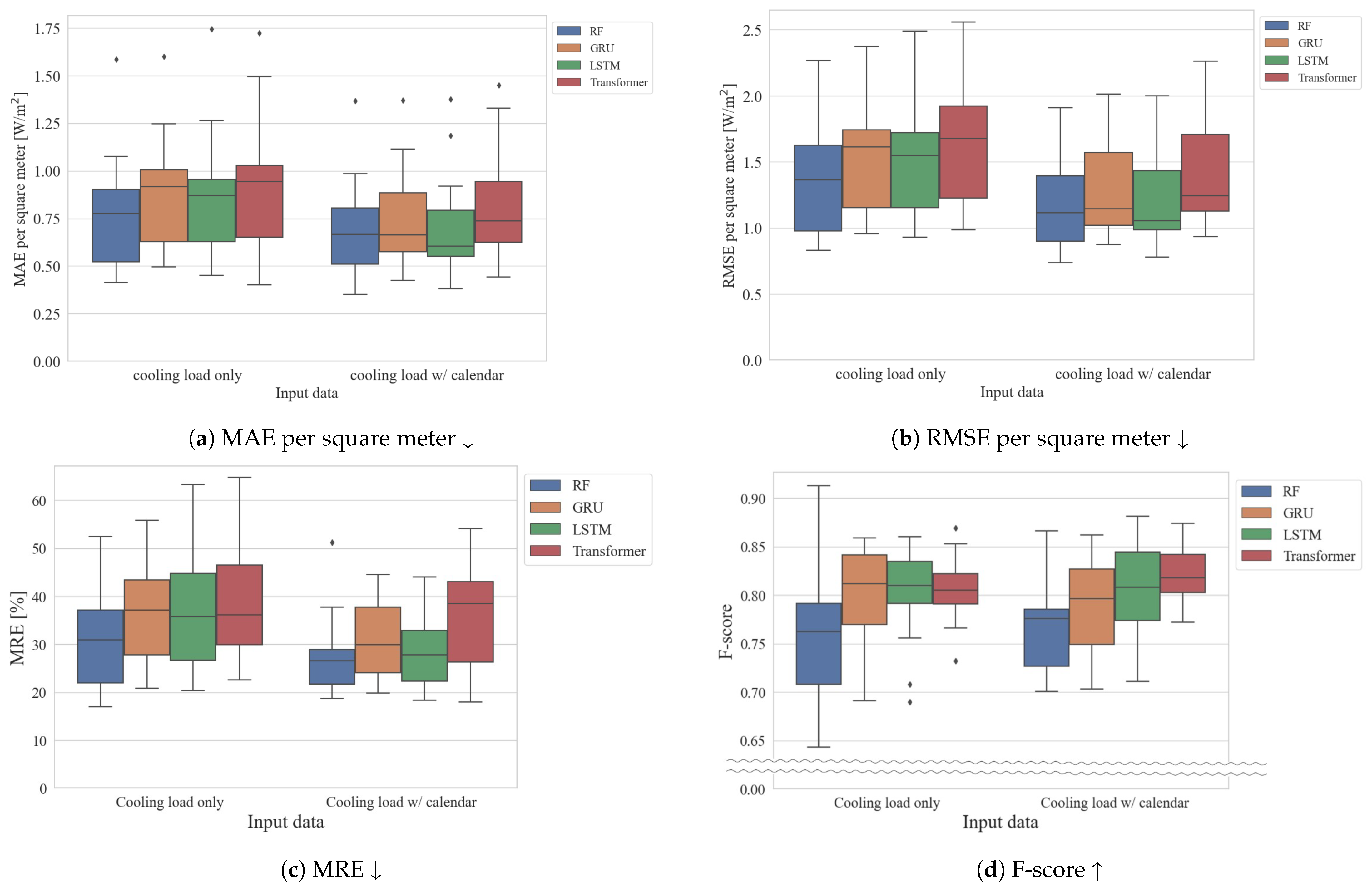
Figure 7 shows the evaluation results for each model across all buildings, evaluated by the MAE, RMSE, MRE, and F-score. In each figure, the box plots represent the models, with blue indicating RF, orange indicating GRU, green indicating LSTM, and red indicating Transformer. In addition, the left side box plots in each figure represent results when only the cooling load was input, while the right side includes calendar information in addition to the cooling load as inputs. The top left is for the MAE, the top right is for the RMSE, the bottom left is for the MRE, and the bottom right is for the F-score. It can also be seen that for the MAE and RMSE, the values of the MAE and RMSE increase proportionally as the area of each building increases because the occupancy density is constant in each building. Therefore, after calculating the MAE and RMSE for each building, these are divided by the office area of the respective building, calculating the MAE and RMSE per square meter, which are then plotted in the box plots.
Initial observations indicate that including calendar information along with the total cooling load significantly improves accuracy. Comparing the median values among the same input models, we observe that, for the MAE and RMSE, the order of error from lowest to highest is LSTM, RF, GRU, and Transformer. These results mean that LSTM provides the most accurate monitoring among these models. As for the MAE, the variance of the estimation results using the RF input cooling load with the calendar was 0.058, while LSTM using the same input was 0.070. Similar to the MAE, for the RMSE, the variance of the estimation result using the RF input cooling load with the calendar was 0.108, while LSTM using the same input was 0.152. Therefore, the RF model has less variance than LSTM; thus, RF can provide a more stable estimation than the other deep learning models. Conversely, for MRE, the order is RF, LSTM, GRU, and Transformer. For the MRE, RF can provide accurate monitoring with a low MRE as compared with the other learning models. Figure 7d shows that Transformer can estimate the occupancy detection more accurately than the other learning models. Transformer provided stable and accurate occupancy detection in many of the buildings tested. Detailed experimental results for each building are provided in Appendix A.
From the above results, LSTM or RF are a good choice for reducing the error between the estimated occupant load and the actual occupant load. LSTM can estimate the load with higher accuracy compared to RF, while RF is a better choice compared to LSTM if stable estimation results are desired. On the other hand, Transformer is a good choice if the objective is to improve the accuracy of occupancy detection. Compared to previous research [7,8,9] from the other point of view, the datasets in previous research [7,8,9] have a fixed occupancy schedule, whereas our data are based on simulated occupancy schedules defined based on measured HVAC on/off data. LSTM and Transformer are more accurate than RF [7,8] with realistic thermal load data from the perspective of the characteristics of the data.
Table 3 shows the average of the calculation time and memory usage in the test phase, which is the time when the learning model estimates the occupant load. As for the calculation time, RF is the fastest compared to the other learning models. A comparison among the deep learning models shows that the Transformer model results in the fastest calculation time. This is because the Transformer model utilized in our experiment has a simple structure consisting of one or two Encoder layers without a Decoder layer. As for the memory usage, there are similar results with the results of the calculation time. RF utilizes the least amount of memory compared to the other learning models. The Transformer model also uses the least amount of memory among the deep learning models, up to 13.5% less, for the same reason as the results of the calculation time. If NITLM is to be implemented in the HVAC or other edge devices, computational effort such as memory capacity and calculation time should be considered. Typically, the edge devices have an average memory capacity of 1 or 2 GB, indicating that these results in Table 3 are applicable to edge devices. In addition, for real-time control, it is a good choice to use a learning model that can be processed at high speed, such as RF.
4.3.2. Comparison between Floors
Table 4 shows the evaluation results based on the MRE when performing estimations using different learning models in Building O. When comparing the results for the 2nd and 6th floors within the same model, the MRE is almost unchanged, varying from 0.97 to 1.22 times. Therefore, there is not much difference in the decomposition accuracy due to the floor level. However, when comparing the 2nd and 8th floors in Table 4, the MRE increases significantly for all models, ranging from 1.9 to 3.0 times. As expected, changes in the number of floors and occupancy patterns produce large changes in the MRE between these floors. Note that if the occupancy pattern differs notably from one floor to another, this will have a significant impact on the MRE in the estimation.
Figure 8 shows heatmaps of the occupancy patterns for the 2nd, 6th, and 8th floors of Building O during the summer of 2019 over four months, with the left figure representing the 2nd floor, the middle figure representing the 6th floor, and the right figure representing the 8th floor. In each heat map, the horizontal axis represents the time of day, and the vertical axis represents individual days over the four months. The maps show the thermal load from occupancy at each time, with darker blue representing a higher occupant load and yellow representing a minimal load. The heat map for the 2nd floor shows a schedule where people arrive around 8 AM and gradually leave after 8 PM. During office hours from 8 AM to 8 PM, the color is mostly dark blue, indicating a steady daily occupant load. This suggests a regular occupancy pattern with almost the same number of occupants each day. Comparing the occupancy patterns on the 2nd and 6th floors, where the MREs are almost the same, the patterns during four months in summer are almost identical. In contrast, the 8th floor shows varying numbers of occupants at different times, with some weeks having more people and others having fewer. Such patterns lead to larger errors in the decomposition compared to the regular pattern of the 2nd floor. However, in the real world, occupancy patterns like the one on the 8th floor are more realistic than the one on the 2nd floor. Therefore, learning models that can accurately capture such varied occupancy patterns are needed.
5. Conclusions and Future Remarks
In this study, we evaluated the accuracy of deep learning models for five buildings with 16 floors using RF, LSTM, GRU, and Transformer. We compared the models for accuracy differences and variance in NITLM accuracy across buildings and floors. Our results showed that including calendar information with the total heat load as input generally improved the overall model accuracy. For reducing occupancy count errors, LSTM was found to be the most suitable choice. However, for increased accuracy stability, it is preferable to use RF due to its smaller variance. For optimal enhancement of occupancy detection accuracy, Transformer is ideal. Additionally, our evaluation of inter-floor differences revealed that variations in accuracy are a result of occupancy patterns unique to each floor, rather than differences in floor levels having a significant impact on accuracy. Our fundamental evaluation results and insights from these results are useful for improving learning models for NITLM tasks.
However, it is important to consider various factors such as building materials and adjacent buildings in real-world scenarios. To develop high-precision disaggregation models, it is necessary to adapt and selectively apply learning models based on the specific conditions of each building. Therefore, future work should clarify the building elements, such as the floor level, window area, or exterior material, that contribute to the differences in accuracy between buildings and floors.
Author Contributions
Conceptualization, K.O., D.Z., H.N. and I.T.; methodology, K.O., N.K., D.Z., H.N. and I.T.; software, K.O. and N.K.; validation, K.O.; formal analysis, K.O.; investigation, K.O. and N.K.; resources, K.O. and N.K.; data curation, K.O. and N.K.; writing—original draft preparation, K.O.; writing—review and editing, N.K., D.Z., H.N., I.T. and F.C.; visualization, K.O.; supervision, D.Z., H.N., I.T. and T.O.; project administration, I.T. All authors have read and agreed to the published version of the manuscript.
Funding
This work was supported by JSPS KAKENHI Grant Number JP22H03697 and DAIKIN Industries, Ltd.
Data Availability Statement
All the data are confidential and cannot be disclosed. We would be willing to share the knowledge and parts of the data to replicate the experiment on a request basis.
Acknowledgments
The authors would like to thank Hiroyuki Murayama, Yoshinori Yura, and Masakazu Okamoto for technical assistance with preparing the dataset and suggesting the topic of this paper.
Conflicts of Interest
Okazawa. K, Kaneko. N, Zhao. D, Nishikawa. H, and Taniguchi. I have received research grants from DAIKIN Industries, Ltd.
Appendix A
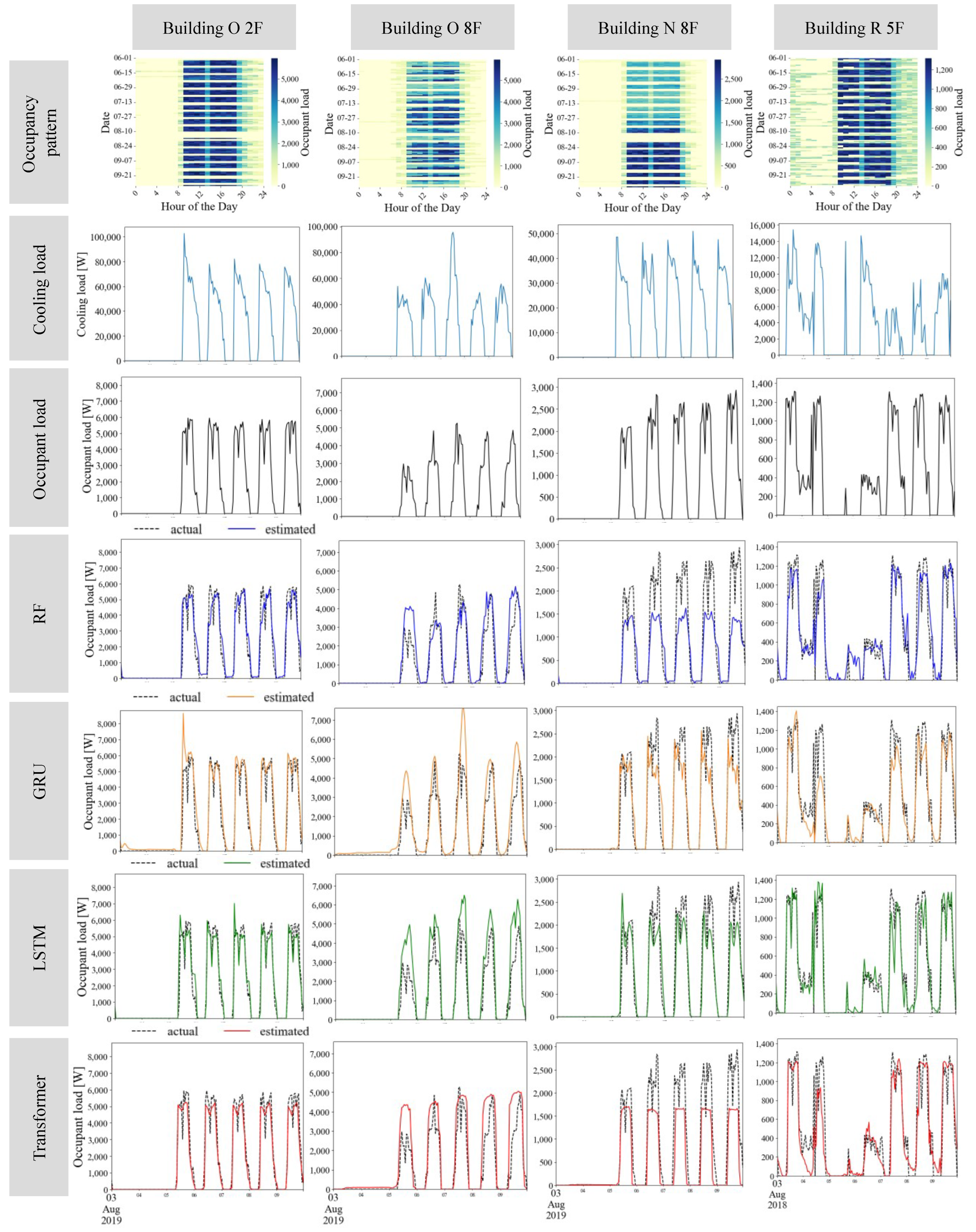
This appendix presents the results estimated for various occupancy patterns when decomposing the thermal load. Figure A1, from the top, shows the occupancy patterns over four months, the actual cooling load and occupant load from 3 August to 9 August, and the estimated results for RF, GRU, LSTM, and Transformer. The heatmap indicating occupancy patterns represents each date on the vertical axis and each time on the horizontal axis. Each time slot indicates the occupant load. Darker colors represent a higher occupant load, while lighter colors represent a smaller occupant load. In the other graphs, the x-axis represents the time, and the y-axis represents the thermal load, such as the cooling load and the occupant load. The estimation results are depicted with black dotted lines for the actual cooling load and blue for RF, orange for GRU, green for LSTM, and red for Transformer estimations. As for the buildings and floors, four types with distinctive occupancy patterns were selected out of sixteen. The occupancy patterns for the four buildings/floors are as follows:
- Building O 2F: On this floor, there are fixed office hours, and the number of people coming in daily is constant. In this case, the daily occupancy patterns do not vary significantly.
- Building O 8F: On this floor, while the office hours are fixed, the number of people coming in varies day-to-day. In this case, unlike Building O 2F, the daily occupancy patterns change significantly.
- Building N 8F: On this floor, there are fixed office hours, and the number of people coming in daily is constant. However, towards the end of July, the number of people coming to this floor increases and remains until the end of September.
- Building R 5F: On this floor, while there are fixed office hours, occupants are present even during late nights and on weekends. Furthermore, since the number of occupants varies day-by-day, the occupancy pattern is irregular compared to the other three floors.
Due to the data collection period for the on/off data of the HVAC system, the data for the 2nd and 8th floors of Building O and the 8th floor of Building N are from 2019, while the data for the 5th floor of Building R are from 2018. Therefore, the first three buildings show a week starting from Saturday, 3 August, while Building R’s data begin from Friday, 3 August in these figures.
When examining the estimation results by building and floor, we can see that, for the second and eighth floors of Building O, although the GRU model sometimes significantly deviates from the actual values, other models accurately follow the actual values. In cases like the eighth floor of Building N, where the number of occupants significantly changes over time, the RF and Transformer models produce estimates lower than the actual values, while the GRU and LSTM models are able to follow the actual values. This indicates that GRU and LSTM can adapt to sudden changes in the number of occupants because they can consider past time-series data. Finally, for the fifth floor of Building R, although all models follow the waveform, if we focus on the brief peaks during the night and on Sundays, there are parts where the waveform is not captured. Considering this, it is evident that, among the learning models, LSTM most accurately follows the waveform.
Figure A1.
Actual cooling load, occupant load, and examples of estimation results using RF, GRU, LSTM, and Transformer for some buildings.
Figure A1.
Actual cooling load, occupant load, and examples of estimation results using RF, GRU, LSTM, and Transformer for some buildings.

References
- Verma, A.; Anwar, A.; Mahmud, M.A.; Ahmed, M.; Kouzani, A. A Comprehensive Review on the NILM Algorithms for Energy Disaggregation. arXiv 2021, arXiv:2102.12578. [Google Scholar]
- Faustine, A.; Mvungi, N.H.; Kaijage, S.; Michael, K. A Survey on Non-Intrusive Load Monitoring Methodies and Techniques for Energy Disaggregation Problem. arXiv 2017, arXiv:1703.00785. [Google Scholar]
- IEA. 2020 Global Status Report for Buildings and Construction; IEA: Paris, France, 2020. [Google Scholar]
- Fischer, C. Feedback on Household Electricity Consumption: A Tool for Saving Energy? Energy Effic. 2008, 1, 79–104. [Google Scholar] [CrossRef]
- Ridi, A.; Gisler, C.; Hennebert, J. A Survey on Intrusive Load Monitoring for Appliance Recognition. In Proceedings of the 2014 22nd International Conference on Pattern Recognition, Stockholm, Sweden, 24–28 August 2014; pp. 3702–3707. [Google Scholar]
- Hart, G.W. Nonintrusive Appliance Load Monitoring. Proc. IEEE 1992, 80, 1870–1891. [Google Scholar] [CrossRef]
- Xiao, Z.; Gang, W.; Yuan, J.; Zhang, Y.; Fan, C. Cooling Load Disaggregation Using a NILM Method Based on Random Forest for Smart Buildings. Sustain. Cities Soc. 2021, 74, 103202. [Google Scholar] [CrossRef]
- Xiao, Z.; Fan, C.; Yuan, J.; Xu, X.; Gang, W. Comparison Between Artificial Neural Network and Random Forest for Effective Disaggregation of Building Cooling Load. Case Stud. Therm. Eng. 2021, 28, 101589. [Google Scholar] [CrossRef]
- Lin, X.; Tian, Z.; Lu, Y.; Zhang, H.; Niu, J. Short-Term Forecast Model of Cooling Load Using Load Component Disaggregation. Appl. Therm. Eng. 2019, 157, 113630. [Google Scholar] [CrossRef]
- Enríquez, R.; Jiménez, M.J.; Heras, M.R. Towards Non-Intrusive Thermal Load Monitoring of Buildings: BES Calibration. Appl. Energy 2017, 191, 44–54. [Google Scholar] [CrossRef]
- Okazawa, K.; Kaneko, N.; Zhao, D.; Nishikawa, H.; Taniguchi, I.; Onoye, T. Exploring of Recursive Model-Based Non-Intrusive Thermal Load Monitoring for Building Cooling Load. In Proceedings of the 14th ACM International Conference on Future Energy Systems, Association for Computing Machinery, Orlando, FL, USA, 20–23 June 2023; pp. 120–124. [Google Scholar]
- Kim, H.; Marwah, M.; Arlitt, M.; Lyon, G.; Han, J. Unsupervised Disaggregation of Low Frequency Power Measurements. In Proceedings of the 2011 SIAM International Conference on Data Mining (SDM), Mesa, AZ, USA, 28–30 April 2011; Society for Industrial and Applied Mathematics: Philadelphia, PA, USA, 2011; pp. 747–758. [Google Scholar]
- Lin, Y.H.; Tsai, M.S.; Chen, C.S. Applications of Fuzzy Classification with Fuzzy c-Means Clustering and Optimization Strategies for Load Identification in NILM Systems. In Proceedings of the 2011 IEEE International Conference on Fuzzy Systems (FUZZ-IEEE 2011), Taipei, Taiwan, 27–30 June 2011; pp. 859–866. [Google Scholar]
- Tabatabaei, S.M.; Dick, S.; Xu, W. Toward Non-Intrusive Load Monitoring via Multi-Label Classification. IEEE Trans. Smart Grid 2017, 8, 26–40. [Google Scholar] [CrossRef]
- Wu, X.; Gao, Y.; Jiao, D. Multi-Label Classification Based on Random Forest Algorithm for Non-Intrusive Load Monitoring System. Processes 2019, 7, 337. [Google Scholar] [CrossRef]
- Cavalca, D.L.; Fernandes, R.A. Recurrence Plots and Convolutional Neural Networks Applied to Nonintrusive Load Monitoring. In Proceedings of the 2020 IEEE Power & Energy Society General Meeting (PESGM), Montreal, QC, Canada, 2–6 August 2020; pp. 1–5. [Google Scholar]
- Davies, P.; Dennis, J.; Hansom, J.; Martin, W.; Stankevicius, A.; Ward, L. Deep Neural Networks for Appliance Transient Classification. In Proceedings of the ICASSP 2019—2019 IEEE International Conference on Acoustics, Speech and Signal Processing (ICASSP), Brighton, UK, 12–17 May 2019; pp. 8320–8324. [Google Scholar]
- Athanasiadis, C.; Doukas, D.; Papadopoulos, T.; Chrysopoulos, A. A scalable real-time non-intrusive load monitoring system for the estimation of household appliance power consumption. Energies 2021, 14, 767. [Google Scholar] [CrossRef]
- Le, T.-T.-H.; Kim, J.; Kim, H. Classification Performance Using Gated Recurrent Unit Recurrent Neural Network on Energy Disaggregation. In Proceedings of the 2016 International Conference on Machine Learning and Cybernetics (ICMLC), Jeju, Republic of Korea, 10–13 July 2016; Volume 1, pp. 105–110. [Google Scholar]
- Rafiq, H.; Zhang, H.; Li, H.; Ochani, M.K. Regularized LSTM Based Deep Learning Model: First Step Towards Real-Time Non-Intrusive Load Monitoring. In Proceedings of the 2018 IEEE International Conference on Smart Energy Grid Engineering (SEGE), Oshawa, ON, Canada, 12–15 August 2018; pp. 234–239. [Google Scholar]
- Shi, Y.; Zhao, X.; Zhang, F.; Kong, Y. Non-intrusive load monitoring based on swin-transformer with adaptive scaling recurrence plot. Energies 2022, 15, 7800. [Google Scholar] [CrossRef]
- Egarter, D.; Elmenreich, W. Autonomous Load Disaggregation Approach Based on Active Power Measurements. In Proceedings of the 2015 IEEE International Conference on Pervasive Computing and Communication Workshops (PerCom Workshops), St. Louis, MO, USA, 23–27 March 2015; pp. 293–298. [Google Scholar]
- Kolter, J.Z.; Johnson, M.J. REDD: A Public Data Set for Energy Disaggregation Research. In Proceedings of the Workshop on Data Mining Applications in Sustainability (SIGKDD), San Diego, CA, USA, 21–24 August 2011; Volume 25. [Google Scholar]
- Kelly, J.; Knottenbelt, W. Neural NILM: Deep Neural Networks Applied to Energy Disaggregation. In Proceedings of the ACM International Conference on Embedded Systems for Energy-Efficient Built Environments, Seoul, Republic of Korea, 4–5 November 2015; pp. 55–64. [Google Scholar]
- Zhang, C.; Zhong, M.; Wang, Z.; Goddard, N.; Sutton, C. Sequence-to-Point Learning With Neural Networks for Non-Intrusive Load Monitoring. In Proceedings of the AAAI Conference on Artificial Intelligence, New Orleans, LA, USA, 2–7 February 2018; Volume 32. [Google Scholar]
- Krystalakos, O.; Nalmpantis, C.; Vrakas, D. Sliding Window Approach for Online Energy Disaggregation Using Artificial Neural Networks. In Proceedings of the Hellenic Conference on Artificial Intelligence, Patras, Greece, 9–12 July 2018; pp. 1–6. [Google Scholar]
- Dosovitskiy, A.; Beyer, L.; Kolesnikov, A.; Weissenborn, D.; Zhai, X.; Unterthiner, T.; Dehghani, M.; Minderer, M.; Heigold, G.; Gelly, S.; et al. An Image Is Worth 16x16 Words: Transformers for Image Recognition at Scale. arXiv 2020, arXiv:2010.11929. [Google Scholar]
- Wolf, T.; Debut, L.; Sanh, V.; Chaumond, J.; Delangue, C.; Moi, A.; Cistac, P.; Rault, T.; Louf, R.; Funtowicz, M.; et al. HuggingFace’s Transformers: State-of-the-Art Natural Language Processing. arXiv 2019, arXiv:1910.03771. [Google Scholar]
- Zhou, H.; Zhang, S.; Peng, J.; Zhang, S.; Li, J.; Xiong, H.; Zhang, W. Informer: Beyond Efficient Transformer for Long Sequence Time-Series Forecasting. arXiv 2020, arXiv:012.07436. [Google Scholar] [CrossRef]
- Yue, Z.; Witzig, C.R.; Jorde, D.; Jacobsen, H.A. Bert4NILM: A Bidirectional Transformer Model for Non-Intrusive Load Monitoring. In Proceedings of the 5th International Workshop on Non-Intrusive Load Monitoring, Virtual Event, 18 November 2020; pp. 89–93. [Google Scholar]
- Çavdar, İ.H.; Feryad, V. Efficient design of energy disaggregation model with bert-nilm trained by adax optimization method for smart grid. Energies 2021, 14, 4649. [Google Scholar] [CrossRef]
- Laouali, I.; Ruano, A.; Ruano, M.D.; Bennani, S.D.; Fadili, H.E. Non-intrusive load monitoring of household devices using a hybrid deep learning model through convex hull-based data selection. Energies 2022, 15, 1215. [Google Scholar] [CrossRef]
- Open-Source Software, EnergyPlus. 1996. Available online: https://energyplus.net/ (accessed on 16 April 2023).
- Pytorch, Meta AI, Menlo Park, CA, USA. Available online: https://pytorch.org/ (accessed on 18 April 2024).
- GeForce RTX 3070, Nvidia, Santa Clara, CA, USA. Available online: https://www.nvidia.com/en-us/geforce/graphics-cards/30-series/rtx-3070-3070ti/ (accessed on 18 April 2024).
Figure 1.
Summary of Non-Intrusive Thermal Load Monitoring (NITLM).

Figure 2.
LSTM and GRU architecture.

Figure 3.
Illustration of the thermal load estimation workflow. The learning models estimate the current occupant load based on the current and past cooling load.
Figure 3.
Illustration of the thermal load estimation workflow. The learning models estimate the current occupant load based on the current and past cooling load.


Figure 4.
Floor layout of building models.

Figure 5.
Details of the experimental period.

Figure 6.
The experimental flow.

Figure 7.
Comparison of evaluation metrics between learning models and input data. We evaluated the MAEs and RMSEs per square meter, which are calculated by dividing by the office area of each building because MAEs and RMSEs vary with the area of each building. Diamond sign indicates as outlier and arrows in the caption are whether a higher or lower value indicates a better or worse evaluation metrics.

Figure 8.
Changes in occupancy patterns in Building O.


Table 1.
The details of building models.
| Building | Building O | Building R | Building N | Building A | Building Y |
| Location | Tokyo | Tokyo | Tokyo | Osaka | Osaka |
| Stories | 9 floors | 9 floors | 9 floors | 6 floors | 6 floors |
| Total floor area | Approx. 6900 m2 | Approx. 1000 m2 | Approx. 3600 m2 | Approx. 2400 m2 | Approx. 3700 m2 |
| Target floors | 2∼9 floor (Approx. 600 m2) | 4, 5, 7 floor (Approx. 120 m2) | 8 floor (Approx. 320 m2) | 2 floor: Approx. 200 m2 3 floor: Approx. 150 m2 | 3, 4 floor (Approx. 430 m2) |
| Experiment period | 2018, 2019 1 Jun.∼30 Sep. | 2017, 2018 1 Jun.∼30 Sep. | 2018, 2019 1 Jun.∼30 Sep. | 2018, 2019 1 Jun.∼30 Sep. | 2018, 2019 1 Jun.∼30 Sep. |
Table 2.
Occupancy, lighting, and equipment operating schedules.
| Thermal Load | Occupancy | Lighting | Equipment | |
|---|---|---|---|---|
| Weekday | Maximum | 0.1 person/m2 | 12 W/m2 | 12 W/m2 |
| HVAC ON Schedule | 00:00–08:00 (20%) | 00:00–08:00 (50%) | 00:00–08:00 (25%) | |
| 08:00–12:00 (100%) | 08:00–12:00 (100%) | 08:00–12:00 (100%) | ||
| 12:00–13:00 (60%) | 12:00–13:00 (50%) | 12:00–13:00 (80%) | ||
| 13:00–18:00 (100%) | 13:00–19:00 (100%) | 13:00–18:00 (100%) | ||
| 18:00–19:00 (50%) | 19:00–20:00 (80%) | 18:00–20:00 (50%) | ||
| 19:00–20:00 (30%) | 20:00–24:00 (50%) | 20:00–24:00 (25%) | ||
| 20:00–24:00 (20%) | ||||
| HVAC OFF Schedule | 00:00–24:00 (0%) | 00:00–24:00 (0%) | 00:00–24:00 (25%) | |
| Weekend | HVAC ON Schedule | 00:00–24:00 (25%) | 00:00–24:00 (50%) | 00:00–24:00 (25%) |
| HVAC OFF Schedule | 00:00–24:00 (0%) | 00:00–24:00 (0%) | 00:00–24:00 (25%) |
Table 3.
Comparison of the calculation time [s] and the memory usage in GPUs [MB] between learning models and input data while they estimate the occupant load.
Table 3.
Comparison of the calculation time [s] and the memory usage in GPUs [MB] between learning models and input data while they estimate the occupant load.
| RF | GRU | LSTM | Transformer | ||
|---|---|---|---|---|---|
| Calculation time | Cooling load | 0.0022 | 0.8050 | 0.8163 | 0.6743 |
| Cooling load w/clalender | 0.0024 | 0.8251 | 0.9129 | 0.6762 | |
| Memory usage | Cooling load | 500.4 | 748.6 | 759.1 | 708.4 |
| Cooling load w/clalender | 494.3 | 757.0 | 795.6 | 688.4 |
Table 4.
Comparison of MREs between the floors in Building O.
| RF | GRU | LSTM | Transformer | |
|---|---|---|---|---|
| Building O 2F | 19.0 | 20.5 | 18.7 | 17.9 |
| 3F | 19.7 | 19.9 | 20.9 | 20.2 |
| 4F | 23.4 | 24.1 | 23.6 | 26.4 |
| 5F | 18.7 | 25.2 | 21.5 | 25.7 |
| 6F | 18.8 | 19.8 | 18.3 | 21.9 |
| 7F | 28.1 | 28.4 | 26.4 | 41.3 |
| 8F | 35.3 | 44.5 | 44.0 | 54.0 |
| 9F | 27.2 | 36.8 | 29.2 | 52.8 |
Disclaimer/Publisher’s Note: The statements, opinions and data contained in all publications are solely those of the individual author(s) and contributor(s) and not of MDPI and/or the editor(s). MDPI and/or the editor(s) disclaim responsibility for any injury to people or property resulting from any ideas, methods, instructions or products referred to in the content. |
© 2024 by the authors. Licensee MDPI, Basel, Switzerland. This article is an open access article distributed under the terms and conditions of the Creative Commons Attribution (CC BY) license (https://creativecommons.org/licenses/by/4.0/).
Share and Cite
MDPI and ACS Style
Okazawa, K.; Kaneko, N.; Zhao, D.; Nishikawa, H.; Taniguchi, I.; Catthoor, F.; Onoye, T. Evaluation of Deep Learning-Based Non-Intrusive Thermal Load Monitoring. Energies 2024, 17, 2012. https://doi.org/10.3390/en17092012
AMA Style
Okazawa K, Kaneko N, Zhao D, Nishikawa H, Taniguchi I, Catthoor F, Onoye T. Evaluation of Deep Learning-Based Non-Intrusive Thermal Load Monitoring. Energies. 2024; 17(9):2012. https://doi.org/10.3390/en17092012
Chicago/Turabian StyleOkazawa, Kazuki, Naoya Kaneko, Dafang Zhao, Hiroki Nishikawa, Ittetsu Taniguchi, Francky Catthoor, and Takao Onoye. 2024. "Evaluation of Deep Learning-Based Non-Intrusive Thermal Load Monitoring" Energies 17, no. 9: 2012. https://doi.org/10.3390/en17092012
Note that from the first issue of 2016, this journal uses article numbers instead of page numbers. See further details here.