The Isomorphic Version of Brualdi’s and Sanderson’s Nestedness

Abstract

The discrepancy BR for an $m\times n$ $0,1$-matrix from Brualdi and Sanderson in 1998 is defined as the minimum number of 1 s that need to be shifted in each row to the left to achieve its Ferrers matrix, i.e., each row consists of consecutive 1 s followed by consecutive 0 s. For ecological bipartite networks, BR describes a nested set of relationships. Since two different labelled networks can be isomorphic, but possess different discrepancies due to different adjacency matrices, we define a metric determining the minimum discrepancy in an isomorphic class. We give a reduction to $k\le n$ minimum weighted perfect matching problems. We show on 289 ecological matrices (given as a benchmark by Atmar and Patterson in 1995) that classical discrepancy can underestimate the nestedness by up to $30\%.$

1. Introduction

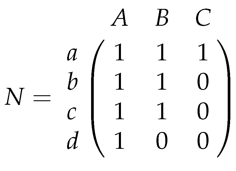
In applied fields like ecology, a $0,1$-matrix M often represents the presence or absence of certain relationships between species or objects, for example, which bee species pollinates which plants or the occurrence and absence of species on several islands. M is often called a contingency table. Such a matrix M can represent a bipartite graph (A bipartite graph $G=(U,V,E)$ consists of two disjoint vertex sets U and V such that all edges are of the form $\{u,v\}$, where $u\in U$ and $v\in V$). Connections of bees and plants are given by edges. Matrix M is then called a bi-adjacency matrix. (For a bipartite graph $G=(U,V,E)$ with $m:=\left|U\right|$ and $n:=\left|V\right|$, we construct its $m\times n$ bi-adjacency matrix M as follows: rows $1,\cdots ,m$ represent vertices $u_1,\cdots ,u_m$ in U, and columns $1,\cdots ,n$ correspond to vertices $v_1,\cdots ,v_n$ in $V.$ If edge $\{u_i,v_j\}\in E$, then we set $M_{i,j}=1$; otherwise, we have $M_{i,j}=0.$) Ecologists call a matrix nested if we find for every row pair $i,j$ in M the following condition; if i has equal or a smaller number of 1 s than j then $M_{i,k}=1$ if and only if $M_{j,k}=1.$ Consider in Figure 1 the nested matrix N that represents the relationships between bee and plant species, and their corresponding bipartite graph.

The term nestedness has already been introduced in 1937 by Hultén [1]. A comprehensive history, discussion, and a definition of nestedness is given by Ulrich et al. [2]. They describe nestedness as follows: “In a nested pattern, the species composition of small assemblages is a nested subset of the species composition of large assemblages”. Interpreting nestedness regarding biological properties in networks is quite interesting. In matrix N of Figure 1 bees b, c, and d pollinate less plants than bee a. However, it does not happen that these bees pollinate other plants than bee a. In a nested matrix, we find, for an arbitrary pair of bee species, that the bee species with less than or an equal number of pollinated plants always pollinates a subset of the plant species that is pollinated from the other one. Hence, it cannot happen that a specialized bee pollinates other plants than a bee which pollinates more plant species. An opposite scenario is that all bee pairs pollinate pairwise different plants like in matrix M of Example 1.

Example 1.

Matrix $M=\begin{array}{cc}& \begin{array}{cccc}A& B& C& D\end{array}\\ \begin{array}{c}a\\ b\\ c\end{array}& \left(\begin{array}{cccc}1& 0& 0& 1\\ 0& 1& 0& 0\\ 0& 0& 1& 0\end{array}\right)\end{array}$ is not nested since each bee pollinates a different plant than every other bee.

Imagine the extinction of a specialized bee in a nested matrix. Since this bee only pollinates plants, which are also pollinated from more generalized bees (bees which pollinate more plants), the pollination for all plants is still preserved. Even the extinction of a generalized bee would preserve the pollination of plants that are still pollinated by specialized bees. In contrast, the extinction of bee a in matrix M of Example 1 would lead to the extinction of plants A and D because no other bee can provide this service for these plants. Real data matrices are mostly not nested (which can be seen in our experimental Section 3). However, it seems that understanding “how much” ecological matrices are nested is important due to the fact that nestedness has been suggested as key to the stability of complex ecological systems. More information about stability and nestedness can be found, for example, in the following articles [3,4,5,6].

Notice that it is always possible to exchange columns and rows in a given matrix such that one finds non-increasing column and row sums. This indeed results in a different matrix. Anyway, it contains exactly the same relationships as before, and let us consider Example 2.

Example 2.

Exchanging columns 2 and 3 in matrix N of Figure 1 leads to matrix $N^{\prime }=\begin{array}{cc}& \begin{array}{ccc}A& C& B\end{array}\\ \begin{array}{c}a\\ b\\ c\\ d\end{array}& \left(\begin{array}{ccc}1& 1& 1\\ 1& 0& 1\\ 1& 0& 1\\ 1& 0& 0\end{array}\right)\end{array},$ which does not fulfill the property of non-increasing column sums. Moreover, in this matrix, it is more difficult to recognize nestedness because rows 2, 3 and 4 do not consist of consecutive 1 s followed by consecutive 0 s.

However, if columns and rows are ordered in regards to non-increasing row and column sums, it is easy to decide whether a given matrix is nested or not. We give a mathematical definition for nestedness.

Definition 1 (nestedness).

Let M be an $m\times n$ $0,1$-matrix where the columns $1,\cdots ,n$ and rows $1,\cdots ,m$ are sorted such that we find for the column sums $c_1\ge c_2\ge \cdots \ge c_n$, and for the row sums $s_1\ge s_2\ge \cdots \ge s_m.$ Then, matrix M is callednestedif and only if each of the m rows start with consecutive 1 s followed by consecutive 0 s.

In graph theory, a nested matrix is usually referred to as Ferrers matrix [7]. We will use equivalently the two terms. Moreover, a whole theory around Ferrers matrices exists, and it is worth reconsidering theoretical insights regarding the nestedness metrics. Let M be an $m\times n$ $0,1$-matrix with non-increasing row sums $(r_1,\cdots ,r_m)$ and non-increasing column sums $(c_1,\cdots ,c_n).$ The corresponding Ferrers matrixF is the matrix where each row i of F starts with $r_i$ 1 s followed by $n-r_i$ 0 s. It can be achieved in several shifts. A shift is the movement of a 1 in a row from a right to a left column with entry $0,$ i.e., it is an exchange of entries $M_{i,j}=1$ and $M_{i,j^{\prime }}=0$ for $j>j^{\prime }$ leading to the matrix $M^{\prime }$ with $M_{i,j}^{\prime }=0$, $M_{i,j^{\prime }}^{\prime }=1$ and $M_{k,\ell }^{\prime }=M_{k,\ell }$ for all index pairs of M with $(k,\ell )\ne (i,j)$ or $(k,\ell )\ne (i,j^{\prime }).$ The corresponding Ferrers matrix of matrix M in Example 1 can be seen in Example 3.

Example 3.

Matrix $F=\begin{array}{cc}& \begin{array}{cccc}A& B& C& D\end{array}\\ \begin{array}{c}a\\ b\\ c\end{array}& \left(\begin{array}{cccc}1& 1& 0& 0\\ 1& 0& 0& 0\\ 1& 0& 0& 0\end{array}\right)\end{array}$ is the corresponding Ferrers matrix of matrix M in Example 1. It can be achieved by shifting 1 s to the left. Matrix F has the same row sums like M but different column sums.

Example 3 shows that Ferrers matrix F has the same row sums as M but different column sums. They can be calculated in counting for each row i in M the number of rows which have at least row sum $i.$

Remark 1.

Let M be an $m\times n$ $0,1$-matrix M where the columns $1,\cdots ,n$ and rows $1,\cdots ,m$ are sorted such that we find for the column sums $c_1\ge c_2\ge \cdots \ge c_n$, and for the row sums $s_1\ge s_2\ge \cdots \ge s_m.$ Furthermore, let F be its corresponding Ferrers matrix. Then, Matrix F also has row sums $(r_1,\cdots ,r_n)$ but different column sums, i.e., $(c_1^{\prime },\cdots ,c_n^{\prime }),$ where $c_i^{\prime }=\left|\left\{j\right|j\mathrm{is}\mathrm{row}\mathrm{in}\mathrm{M}\mathrm{with}{r}_j\ge i\}\right|.$

Remark 1 gives row and column sums for a corresponding Ferrers matrix F of $M.$ The vector $(c_1^{\prime },\cdots ,c_n^{\prime })$ of column sums is also known as conjugate vector of $(r_1,\cdots ,r_n).$ Furthermore, it is a classical result that there is exactly one matrix with these column and row sums [8] (Section 2).

Remark 2.

The corresponding Ferrers matrix F of a matrix M is unique.

Ferrers matrices together with majorisation theory are classical concepts for deciding the question: whether a matrix M (or its bipartite graph) exists with given row and column sums. When matrix M is interpreted as the bi-adjacency matrix, then the corresponding graph of matrix F (considered now as bi-adjacency matrix) is then a threshold graph. For an overview about these problems, we recommend Brualdi’s book [9] or Mahadev’s and Peled’s book [10].

In most real world data, a matrix M is not nested. Hence, the natural question arises of “how far the ecological matrix is from being nested”. Brualdi and Sanderson answered this question with the metrics of discrepancy $disc\left(M\right)$ [11]. (In ecology, it is common to use the notion BR instead of $disc$ [2]). It is based on the fact that every matrix M has a unique Ferrers matrix F that can be achieved by shifting 1 s in each row from larger to smaller column indices with entry 0 (see Remark 2). The discrepancy of a given matrix M is the minimum number of shifts of 1 s to the left required to achieve its Ferrers matrix. A value of 0 represents a nested matrix. This means that the the larger the discrepancy is (the more shifts are needed to yield the Ferrers matrix), the less a matrix is nested. Hence, the discrepancy metrics measures the strength to be non-nested. Consider matrix M in Example 4 and its unique Ferrers matrix F. In the first row, it is possible to shift the 1 in the third column to the second column, and the 1 of the fourth column to the third one. However, one only needs a single shift, i.e., moving the 1 of the fourth column to the second one. Following this approach for each row, we find $disc\left(M\right)=4.$ The discrepancy can be easily calculated. However, there is a conceptual problem when applied to an ecological data set. Exchanging two different columns i and $i^{\prime }$ in $M,$ holding the same column sums, leads to another matrix $M^{\prime }$ with $M\ne M^{\prime }.$ The values of the discrepancy for M and $M^{\prime }$ can be different. However, both bi-adjacency matrices represent exactly the same relationships between bees and plants. Moreover, these bi-adjacency matrices correspond to two different labelled bipartite graphs. (A graph is labelled if all vertices in vertex set V are indexed by a unique number, i.e., V consists of vertices $v:1,\cdots ,v_n$ where $n:=\left|V\right|.$) Their structure, however, is exactly the same. Formally, those graphs are called isomorphic. (Two labelled graphs $G=(V,E)$ and $G^{\prime }=(V,E^{\prime })$ are called isomorphic if there exists a permutation $\sigma :V\mapsto V$ of vertex labels such that edge $\{v_i,v_j\}\in E$ if and only if $\{v_{\sigma \left(i\right)},v_{\sigma \left(j\right)}\}\in E^{\prime }$.) Consider Example 4.

Example 4.

Bi-adjacency matrices $M:=\begin{array}{cc}& \begin{array}{cccc}A& B& C& D\end{array}\\ \begin{array}{c}a\\ b\\ c\\ d\\ e\\ f\end{array}& \left(\begin{array}{cccc}1& \mathbf{0}& 1& \mathbf{1}\\ 1& \mathbf{0}& 1& \mathbf{1}\\ 1& 1& \mathbf{0}& \mathbf{1}\\ 1& 1& 0& 0\\ 1& 1& 0& 0\\ 1& \mathbf{0}& \mathbf{1}& 0\end{array}\right)\end{array}$ and $M^{\prime }:=\begin{array}{cc}& \begin{array}{cccc}A& B& C& D\end{array}\\ \begin{array}{c}a\\ b\\ c\\ d\\ e\\ f\end{array}& \left(\begin{array}{cccc}1& \mathbf{0}& 1& \mathbf{1}\\ 1& \mathbf{0}& 1& \mathbf{1}\\ 1& 1& 1& 0\\ 1& 1& 0& 0\\ 1& 1& 0& 0\\ 1& \mathbf{0}& 0& 1\end{array}\right)\end{array}$ represent two isomorphic bipartite graphs, i.e., both graphs look the same but plants C and D have in M column indices 3 and 4, whereas in matrix $M^{\prime }$ plant C and D are labelled with 4 and $3.$ Moreover, in M, we need to shift the four bold 1 s to achieve its corresponding Ferrers matrix $F=\left(\begin{array}{cccc}1& 1& 1& 0\\ 1& 1& 1& 0\\ 1& 1& 1& 0\\ 1& 1& 0& 0\\ 1& 1& 0& 0\\ 1& 1& 0& 0\end{array}\right)$, i.e., $disc\left(M\right)=4.$ In matrix $M^{\prime }$, we only need to shift three 1 s to achieve F leading to $disc\left(M^{\prime }\right)=3.$

For ecological purposes, these labels are not necessary. They are only assigned to columns and rows due to the mathematical denotation of columns and rows. The value of the discrepancy is dependent on a “random” order of bees and pollinators in a data set, and its resulting order of columns and rows in its bi-adjacency matrix.

We propose an extended metric based on the discrepancy to repair this problem. We define for a matrix M set $\mathcal{M},$ which contains all matrices that can be achieved by permuting in M columns and rows with identical sums. (Notice, if we consider all matrices in $\mathcal{M}$ as bi-adjacency matrices, then the corresponding set of bipartite graphs is isomorphic. Consider a bipartite graph $G=(U,V,E)$ in this set. The definition of isomorphic graphs allows only the permutation of vertex labels with the same vertex degree in U or $V.$ This corresponds to the permutation of columns and rows in the corresponding bi-adjacency matrix with the same sums.) However, changing the row order in M would not change the discrepancy of M because the number of minimal shifts in each row stays the same. Finding an optimal labelling for a given bipartite graph $G,$ such that its bi-adjacency matrix has a minimum discrepancy under all bi-adjacency matrices of isomorphic graphs of $G,$ can be done by only permuting the columns of its bi-adjacency matrix. We define the isomorphic discrepancy of M as the minimum number of shifts under all matrices in $\mathcal{M}$ to achieve F. In other words, the isomorphic discrepancy finds an optimal labelling for a bipartite graph regarding a minimum number of shifts in its bi-adjacency matrix to achieve its nested matrix $F.$ In Example 4, the discrepancy of M would be overestimated or the nestedness be underestimated, respectively.

We show that the isomorphic discrepancy for a matrix M can be calculated in transforming our problem into less than nminimum perfect weighted matching problems in a bipartite graph. (Given a bipartite graph, $G=(U,V,E)$ with $\left|U\right|=\left|V\right|,$ and weight function $w:E\mapsto \mathbb{R}.$ The perfect matching problem asks for a subset $M\subset E$ of edges such that each vertex of G is in exactly one edge of $M.$ The minimum perfect weighted matching problem asks for a perfect matching M minimizing $w\left(M\right)={\sum }_{m_i\in M}w\left(m_i\right).$) More clearly, we construct for each fixed column sum s a bipartite graph $G_s$ separately. Each edge $\{u_i,v_j\}$ in a minimum perfect weighted matching of $G_s$ tells us that column i in matrix M needs to be moved on position $j.$ In the resulting matrix, all columns with sum s are reordered without violating the non-increasing column sums property. We repeat this approach whenever there exist at least two columns with the same column sum. The resulting matrix is a matrix in $I_M$ with a minimum discrepancy. One of the most important books about matching theory is from Lovász and Plummer [12]. One suitable algorithm for our scenario is from Gabow [13], which achieves an $O\left(n^3\right)$ asymptotic running time, if we follow our approach.

Please observe that there exist other approaches and assumptions of what a nested matrix N for M has to look like. One approach is to find an $M^{\prime }\in \mathcal{M}$ such that a minimal number of 0 s can be replaced by 1 s to become nested. This problem is known as the minimal chain completion problem and was shown to be NP-complete in 1981 by Yannakakis [14]. (It is an open problem whether there is an algorithm to find a solution in polynomial asymptotic running time for NP-complete problems. For more information consider the classical book of Garey and Johnson [15].) The opposite problem is to delete a minimal number of 0s in $M^{\prime }\in \mathcal{M}$ to achieve a nested matrix that is also NP-complete (exchange the rules of 1 s and 0 s to see this). An approximation algorithm was given in the Phd-thesis of Juntilla in 2011 [16]. There are different definitions of nestedness in the ecological community, and several procedures to compute it. For an overview, see the nestedness guide [2] which also includes the discrepancy of Brualdi and Sanderson (there called BR). In the next section, we give a formal definition of isomorphic discrepancy, and show how it can be calculated in asymptotic running time $O\left(n^3\right).$

2. The Discrepancy Problem for Isomorphic Matrices

Let M be an $m\times n$ bi-adjacency matrix with non-increasing row sums $(r_1,\cdots ,r_m)$, and non-increasing column sums $(c_1,\cdots ,c_n),$ and G the corresponding bipartite graph. Furthermore, let $\mathcal{G}$ be the set of all isomorphic graphs of $G.$ Then, all bi-adjacency matrices corresponding to a graph $G^{\prime }\in \mathcal{G}$ can be achieved by permuting columns and rows with equal sums in M. We denote the set of these matrices by $\mathcal{M}.$ The discrepancy of M given by Brualdi and Sanderson [17] is the minimum number of shifts to achieve the corresponding Ferrers matrix F as described in the last section. We denote the discrepancy of M by $disc\left(M\right)$. We now give the definition of the isomorphic discrepancy $Id\left(M\right)$ of M, which is defined by

$$Id\left(M\right):=mi{n}_{B\in \mathcal{M}}disc\left(B\right).$$

(1)

In other words, we try to find a matrix in $\mathcal{M}$ with minimal discrepancy. We also want to mention that this new metric should be invariant against the transposition of $M.$ This can be achieved by transposing M to its transposed matrix $M^t$ and determining $Id\left(M^t\right).$ The general isomorphic discrepancy of M is then the minimum value (or the mean value) of $Id\left(M\right)$ and $Id\left(M^t\right).$ We here focus on $Id\left(M\right)$ because the calculation of $Id\left(M^t\right)$ can be done analogously.

A simple approach is to permute all columns and rows with equal sums, and to choose a permutation of M that yields the minimum discrepancy. This can lead to the determination of exponentially many possible permutations. Please observe that it is sufficient for our problem to permute columns in M and keep the rows fixed. The reason is that exchanging the order of rows with the same sums leads to exactly the same discrepancy because the corresponding rows of the Ferrers matrix are identical. Consider our Example 4. It can be seen that each permutation of the first three rows in M or $M^{\prime }$ lead to the same kind of shifts, and so to the same discrepancy as before. Following this approach, we will not necessarily generate all matrices in $\mathcal{M},$ but the subset $I_M$ that consists of all matrices that were yielded by a permutation of columns in M with the same sum. Hence, matrices in $I_M$ possess the whole range of possible discrepancies that occur for matrices in $\mathcal{M}.$ Hence, it is sufficient to permute columns for the calculation of $Id\left(M\right).$ More formally, we find

$$Id\left(M\right)=mi{n}_{B\in \mathcal{M}}disc\left(B\right)=mi{n}_{B\in I_M}disc\left(B\right).$$

(2)

Consider all matrices with row sums $(r_1,\cdots ,r_m)$ and column sums $(c_1,\cdots ,c_n).$ Then, it follows that all of them possess the same unique Ferrers matrix F with column sums $(c_1^{\prime },\cdots ,c_n^{\prime }).$ (Recall that the lists are non-increasing.) Brualdi and Shen showed [11] that there is always one matrix A with row sums $(r_1,\cdots ,r_m)$ and column sums $(c_1,\cdots ,c_n)$ that has minimum possible discrepancy $disc\left(A\right)={\sum }_{j=1}^n{(c_j^{\prime }-c_j)}^{+}$, where ${\left(a\right)}^{+}:=max\{a,0\}$ for $a\in \mathbb{R}.$ Matrix A can be found by moving in F 1 s from columns j with $c_j^{\prime }-c_j>0,$ to columns i with $c_i^{\prime }-c_i<0.$ Consider Example 5.

Example 5.

For matrix $M:=\left(\begin{array}{cccc}1& \mathbf{0}& 1& \mathbf{1}\\ 1& 1& 1& 0\\ 1& 1& \mathbf{0}& \mathbf{1}\\ 1& 1& 0& 0\\ 1& \mathbf{0}& 0& \mathbf{1}\\ 1& \mathbf{0}& \mathbf{1}& 0\end{array}\right),$ we have $disc\left(M\right)=4$, and corresponding Ferrers matrix $F:=\left(\begin{array}{cccc}1& 1& 1& 0\\ 1& 1& 1& 0\\ 1& 1& 1& 0\\ 1& 1& 0& 0\\ 1& 1& 0& 0\\ 1& 1& 0& 0\end{array}\right).$ We construct matrix $A=\left(\begin{array}{cccc}1& 0& 1& 1\\ 1& 0& 1& 1\\ 1& 0& 1& 1\\ 1& 1& 0& 0\\ 1& 1& 0& 0\\ 1& 1& 0& 0\end{array}\right)$ with $disc\left(A\right)={\sum }_{j=1}^n{(c_j^{\prime }-c_j)}^{+}=3$ by shifting three 1 s of the second column in F to the fourth column. However, the minimum discrepancy under all isomorphic matrices of M is 4, i.e., $Id\left(M\right)=4.$ This is true because each permutation σ of the last three columns of M leads to a matrix $M^{\sigma }$ with $disc\left(M^{\sigma }\right)=4.$ A discrepancy of 3 cannot be achieved by a permutation of columns from $M.$

The set of all matrices with row sums $(r_1,\cdots ,r_m)$ and column sums $(c_1,\cdots ,c_n)$ can be partitioned in isomorphic matrix sets ${\mathcal{M}}_i.$ Example 5 shows that not all sets possess a matrix A with minimum possible discrepancy. If this had been the case, we would already know the value $Id\left(M\right)$ for each matrix. Unfortunately, it is not the case.

We want to develop a simple formula to calculate the discrepancy of a given matrix. We need this formula later to devise an approach for the isomorphic version. Notice that a shift in a matrix M will always be applied when $F_{i,j}=1$ and $M_{i,j}=0.$ Since M and F have identical row sums, and due to the construction of F, there must always be an index $j^{\prime }>j$ with $F_{i,j^{\prime }}=0$ and $M_{i,j^{\prime }}=1.$ In matrices of our Examples 4 and 5, we marked these 0 s and 1 s. This means that the number of absences of 1 s in $M,$ when they are present in $F,$ correspond to the number of minimum shifts $disc\left(M\right)$. We define the difference of the jth columns $A_j$ and $A_j^{\prime }$ of $m\times n$ $0,1$-matrices A and $A^{\prime }$ by

$$(A_j-A_j^{\prime }):=\sum _{i=1}^m{(A_{i,j}-A_{i,j}^{\prime })}^{+}.$$

(3)

Back to our problem, we find $(F_j-M_j)\ge c_j^{\prime }-c_j$ for all $j.$ The reason is that a column $F_j$ has $c_j^{\prime }$ 1 s and a column $M_j$ has $c_j$ 1 s. This means that the minimum difference of both columns happens if all 1 s in $M_j$ also occur in $F_j$. Then, $(F_j-M_j)=c_j^{\prime }-c_j.$ Consider in Example 4 the third columns of M, $M^{\prime }$ and $F.$ $M^{\prime }$ has all 1 s of F, whereas M has only two of them. Hence, $F_3-M_3=1>0=c_3^{\prime }-c_3$ but $F_3-M_3^{\prime }=0=c_3^{\prime }-c_3.$ In cases where you find a 1 in $M_j$, which does not occur in $F_j$, this 1 needs to be shifted to a ’left’ column $j^{\prime }$ where F has a 1 and M a $0.$ A 1 from a ’right’ column $j^{″}$ in M has to be shifted to $M_j$ to achieve the $c_j^{\prime }$ 1 s in F. In Example 4, this is the case for $M_{6,3}.$ We put this connection in another formula for the discrepancy.

Proposition 1.

Let M be an $m\times n$ $0,1$-matrix with non-increasing row sums $(r_1,\cdots ,r_m)$ and non-increasing column sums $(c_1,\cdots ,c_n).$ Let F be the corresponding Ferrers matrix. Then, the minimum number of shifts $disc\left(M\right)$ to achieve F from M can be calculated by $disc\left(M\right)={\sum }_{j=1}^n(F_j-M_j)$.

Proof. 

The proof is by induction on the number n of columns. For one column, we have $M=F$ and so $disc\left(M\right)=0$ and $(F_1-M_1)=0.$ We assume that $disc\left(M\right)={\sum }_{j=1}^k(F_j-M_j)$ holds for all matrices with m rows and $k\le n-1$ columns (induction hypothesis IH). Let us now consider a matrix an $m\times n$ matrix $M.$ Notice that $(F_n-M_n)=0$ for each matrix M and its corresponding Ferrers matrix F due to the construction of $F.$ In column $n-1$ of M, we consider the set I of all indices i where $F_{i,n-1}=1$ and $M_{i,n-1}=0.$ Due to the construction of a Ferrers matrix, and since F and M have equal row sums, we find for all $i\in I$ that $F_{i,n}=0$ and $M_{i,n}=1.$ We construct matrix B by exchanging, for all indices $i\in I$, all entries $M_{i,n-1}=0$ to 1, and all corresponding entries $M_{i,n}=1$ to $0.$ Basically, we apply $\left|I\right|$ shifts from the nth column to the $(n-1)$th column. In matrix B, we only find shiftable 1 s in smaller columns than in column n due to our construction. We delete the last column of B and get the $m\times (n-1)$ matrix $B^{\prime }.$ We apply the induction hypothesis on $B^{\prime }.$ Since (a) matrices B and $B^{\prime }$ have exactly the same number of minimal shifts (because in the first $(n-1)$ columns they are completely identical, and B has in the nth column no shiftable 1 s due to our construction), and (b) M has $\left|I\right|$ more shifts (in the nth column) than $B,$ and (c) matrices M and B are identical in the first $n-2$ columns, and M has in the $n-1$th column $\left|I\right|$ more shifts, we get

$$\begin{array}{cc}\hfill disc\left(M\right)-\left|I\right|\stackrel{\left(b\right)}{=}disc\left(B\right)\stackrel{\left(a\right)}{=}disc\left(B^{\prime }\right)\stackrel{IH}{=}\sum _{j=1}^{n-1}{F}_j-B_j^{\prime }=\sum _{j=1}^n{F}_j-B_j& \stackrel{\left(c\right)}{=}\hfill \\ \hfill \sum _{j=1}^{n-2}(F_j-M_j)+(F_{n-1}-M_{n-1}-\left|I\right|)+(F_n-M_n)=\sum _{j=1}^n(F_j-M_j)-\left|I\right|.\end{array}$$

☐

We denote an element of $I_M$ by $M^{\sigma }$ where $\sigma :\{1,\cdots ,n\}\mapsto \{1,\cdots ,n\}$ is a permutation of the columns of M that exchanges columns with same column sums. Recall (Equation (2)) that this approach covers all possible discrepancies that exist in set $\mathcal{M}.$ A permutation $\sigma$ can be divided in the convolution of k permutations ${\sigma }_i$ if M possesses k different column sums, i.e., $(c_1,c_2,\cdots ,c_n)=(x_1,\cdots ,x_1,x_2,\cdots ,x_2,\cdots ,x_k,\cdots ,x_k)$. Each ${\sigma }_i:\{1,\cdots ,n\}\mapsto \{1,\cdots ,n\}$ permutes all columns with column sum $x_i$ independently, and keeps the indices of columns with different sums, i.e., $\sigma ={\circ }_{i=1}^k{\sigma }_i.$ We denote the set of all possible permutations ${\sigma }_i$ by ${\Sigma }_i$, and for all $\sigma$ by $\Sigma .$ For matrix M in Example 4, we get six different matrices in set $I_M$. Each of them is built by a permutation $\sigma ={\sigma }_1\circ {\sigma }_2$ where ${\sigma }_1$ is the identity permutation which keeps the first column on index $1,$ and ${\sigma }_2$ permutes the second, third and fourth columns of $M.$ The same is true for $M^{\prime }$ in Example 4. Notice that, $I_M\cap I_{M^{\prime }}\ne \varnothing .$ Let $s_i$ be the number of columns with column sum $x_i.$ We construct k different $m\times s_i$ sub-matrices $M^i.$ Each of them consists of all columns in M with column sum $x_i.$ We denote the column indices j in $M^i$ by the same indices like in $M,$ i.e., $j\in \{s_1+s_2+\cdots +s_{i-1}+1,\cdots ,s_1+s_2+\cdots +s_{i-1}+s_i\}.$ The next Proposition states that calculating the minimum discrepancy of each matrix $M^i$ can be done separately. The sum of all minimum discrepancies for each $M^i$ is then the minimum discrepancy of $M.$

Proposition 2.

Let M be an $m\times n$ matrix M with non-increasing row sums $(r_1,\cdots ,r_m)$ and non-increasing column sums $(c_1,\cdots ,c_n)=(x_1,\cdots ,x_1,x_2,\cdots ,$ $x_2,\cdots ,x_k,\cdots ,x_k)$. Let F be the corresponding Ferrers matrix of M. Then, the isomorphic discrepancy of matrix M is

$$Id\left(M\right)=\sum _{i=1}^k\left(\underset{{\sigma }_i\in {\Sigma }_i}{min}\sum _{j:c_j=x_i}(F_j-M_j^{{\sigma }_i})\right).$$

Proof. 

Since the isomorphic discrepancy is the minimum discrepancy in the set of all matrices in $I_M$ (Equation (2)), and for each matrix $B\in I_M$ there exists a permutation $\sigma ={\circ }_{i=1}^k{\sigma }_i$ with $\sigma \in \Sigma$ and $B=M^{\sigma },$ we get for the isomorphic discrepancy of M

$$Id\left(M\right)\stackrel{Equation \left(2\right)}{=}mi{n}_{B\in I_M}disc\left(B\right)=mi{n}_{\sigma \in \Sigma }disc\left(M^{\sigma }\right)\stackrel{Proposition 1}{=}\underset{\sigma \in \Sigma }{min}\left(\sum _{j=1}^n(F_j-M_j^{\sigma })\right).$$

(4)

Since each $\sigma$ is the convolution of k permutations ${\sigma }_i$ that permute only the column indices with same sums ($\sigma ={\circ }_{i=1}^k{\sigma }_i$), we can rewrite

$$\left(\sum _{j=1}^n(F_j-M_j^{\sigma })\right)=\sum _{i=1}^k\left(\sum _{j:c_j=x_i}(F_j-M_j^{{\sigma }_i})\right).$$

Together with Equation (4), and since $\sigma$ permutes columns with each fixed sum $x_i$ independently, we get

$$Id\left(M\right)\stackrel{Equation \left(4\right)}{=}\underset{\sigma \in \Sigma }{min}\sum _{i=1}^k\left(\sum _{j:c_j=x_i}(F_j-M_j^{{\sigma }_i})\right)=\sum _{i=1}^k\left(\underset{{\sigma }_i\in {\Sigma }_i}{min}\sum _{j:c_j=x_i}(F_j-M_j^{{\sigma }_i})\right).$$

☐

Proposition 2 states that we need to find for each sub-matrix $M_i$ in M with fixed column sums $x_i$ a column order (a permutation ${\sigma }_i$) that minimizes the following sum:

$$w\left({\sigma }_i\right):=\sum _{j:c_j=x_i}(F_j-M_j^{{\sigma }_i}).$$

(5)

We transform the calculation of $Id\left(M\right)$ for each sub-matrix $M^i$ ($i\in \{1,\cdots ,k\}$) of M to the determination of minimum weighted perfect matching problem in a labelled weighted complete bipartite graph (A bipartite graph $G=(U,V,E)$ is called complete if and only if each pair of vertices $u,v$ with $u\in U$ and $v\in V$ is connected by an edge, i.e., $\{u,v\}\in E.$ If we have a weight function $w:E\mapsto \mathbb{R}$ which assigns to every edge in G a weight, then G is called weighted $G_i=(U_{M^i},V_{F^i},E_i).$). In $G_i$, each vertex $u_j\in U_{M^i}$ corresponds to a column $M_j^i$ of $M^i$ where $j\in \{s_1+s_2+\cdots +s_{i-1}+1,\cdots ,s_1+s_2+\cdots +s_{i-1}+s_i\}.$ Moreover, each vertex $v_j\in V_{F^i}$ corresponds to a column $F_j$ of the Ferrers matrix F of M where $j\in \{s_1+s_2+\cdots +s_{i-1}+1,\cdots ,s_1+s_2+\cdots +s_{i-1}+s_i\},$ i.e., we consider the exactly same indices of columns in F as in sub-matrix $M^i.$ For simplicity we denote vertices $u_j$ by $M_j^i$, or, $v_j$ by $F_j$, respectively. We assign each edge $\{M_j^i,F_{j^{\prime }}\}\in E_i$ the weight $w(M_j^i,F_{j^{\prime }}):=(F_j-M_{j^{\prime }}^i)$. Now, we calculate a minimum weighted perfect matching $P^i=\{\{M_1^i,F_{j_1}\},\cdots ,\{M_{s_i}^i,F_{j_{s_i}}\}\}$ in each $G_i.$ Hence, $P^i$ minimizes Equation (5). Moreover, an edge $\{M_{\ell }^i,F_{j_{\ell }}\}$ in $P^i$ tells us that we have to put column ℓ in M on position $j_{\ell }.$ That is, $P^i$ calculates how to permute the columns in $M^i$ such that the discrepancy is minimal. Consider Example 6.

Example 6.

For the $3\times 5$-matrix $M:=\left(\begin{array}{ccccc}1& 1& 0& 1& 0\\ 0& 1& 1& 0& 0\\ 1& 0& 0& 0& 1\end{array}\right)$ with $disc\left(M\right)=3$, we get $3\times 2$-sub-matrix $M^1:=\left(\begin{array}{cc}1& 1\\ 0& 1\\ 1& 0\end{array}\right)$ with column sums 2, and $3\times 3$-matrix $M^2:=\left(\begin{array}{ccc}0& 1& 0\\ 1& 0& 0\\ 0& 0& 1\end{array}\right)$ with column sums $1.$ Hence, we have to construct two complete bipartite graphs $G_1=(U_{M^1},V_{F^1},E_1)$ and $G_2=(U_{M^2},V_{F^2},E_2).$ The Ferrers matrix for M is $F=\left(\begin{array}{ccccc}1& 1& 1& 0& 0\\ 1& 1& 0& 0& 0\\ 1& 1& 0& 0& 0\end{array}\right).$ We get for $G_1$ vertices $M_1$, $M_2,$ $F_1$, $F_2$, and for $G_2$ vertices $M_3,$ $M_4$, $M_5,$ $F_3$, $F_4$, $F_5$. The edge weights between a vertex $M_j^i$ and $F_{j^{\prime }}$ are $w(F_{j^{\prime }},M_j^i):=(F_{j^{\prime }}-M_j^i).$ This leads in $G_1$ to a weight of 1 for all edges. Hence, every perfect matching $P^1$ in $G^1$ has weight $w\left(P^1\right)=2$, and is minimal. The order of the columns in $M^1$ does not matter. On the contrary, in $G_2$, we find the minimum perfect weighted matching $P^2=\{\{M_3,F_4\},\{M_4,F_3\},\{M_5,F_5\}\}$ of weight $w\left(P^2\right)=0.$ Notice that $w(F_3,M_5)=1$ and $w(F_3,M_3)=1.$ All other weights in $G_2$ are $0.$ Hence, the perfect matching $P^{*}=\{\{M_3,F_3\},\{M_3,F_3\},\{M_5,F_5\}\}$ corresponds to the order of columns in M with weight $w\left(P^{*}\right)=1$, which is not the minimum. We need to exchange columns 3 and 4 in $M.$ We get matrix $M^{\prime }:=\left(\begin{array}{ccccc}1& 1& 1& 0& 0\\ 0& 1& 0& 1& 0\\ 1& 0& 0& 0& 1\end{array}\right)$ with $M^{\prime }\in I_M$ and $disc\left(M^{\prime }\right)=2.$ Notice that $disc\left(M^{\prime }\right)=2$ corresponds to the value $w\left(P^1\right)+w\left(P^2\right)=2.$

Theorem 1.

Calculating the isomorphic distance $Id\left(M\right)$ of an $m\times n$ $0,1$-matrix M needs $O\left(n^3\right)$ asymptotic time.

Proof. 

Let $P^i=\{\{M_1^i,F_{j_1}\},\cdots ,\{M_{s_i}^i,F_{j_{s_i}}\}\}$ be a minimum weighted perfect matching in bipartite graph $G_i$ for each $i\in \{1,\cdots ,k\}.$ Then, permutation ${\sigma }_i:\{1,\cdots ,n\}\mapsto \{1,\cdots ,n\}$ with ${\sigma }_i\left(\ell \right)=j_{\ell }$ for all edges $\{M_{\ell }^i,F_{j_{\ell }}\}\in P^i$, and ${\sigma }_i\left(j\right)=j$ for all j with $c_j\ne x_i$ is a permutation of the columns in sub-matrix $M^i$, which minimizes $w\left({\sigma }_i\right)$ in Equation (5). With Proposition 2, and because the perfect matching has minimum weight, we get for $\sigma :={\circ }_{i=1}^k{\sigma }_i$ that

$$\sum _{i=1}^{k}w\left(P^i\right)\stackrel{Eq.5}{=}\sum _{i=1}^{k}mi{n}_{{\sigma }_i\in {\Sigma }_i}(\sum _{j:c_j=x_i}(F_j-M_j^{{\sigma }_i}))=Id\left(M\right).$$

Let us now assume that each permutation $\sigma$ that minimizes $w\left({\sigma }_1\right),\cdots ,w\left({\sigma }_k\right)$ corresponds in each graph $G_i$ to a perfect matching $P^i$ with $\{M_j,F_{j^{\prime }}\}\in P^i$ if ${\sigma }_i\left(j^{\prime }\right)=j$ for $F_j\in V_{F^i}$ and $M_{j^{\prime }}\in U_{M^i}.$ This matching is by construction minimal.

Let $s_i$ be the number of columns with sum $x_i.$ Then, the computation of a minimum weighted perfect matching in $G_i$ is $O\left(s_i^3\right)$ (see, for example, [13]). Since ${\sum }_{i=1}^k{s}_i^3\le {({\sum }_{i=1}^k{s}_i)}^3=n^3$ (because ${\sum }_{i=1}^k{s}_i=n$), we get a total asymptotic running time of $O\left(n^3\right).$ ☐

Please observe that under certain conditions the construction of several graphs $G_i$ can be avoided. This happens for example when the corresponding Ferrers columns are completely equal like in Example 6 in $G_1$. Then, all edge weights in $G_i$ are also equal, and therefore, each perfect matching is a solution.

3. Discrepancy versus Isomorphic Discrepancy in Ecological Matrices

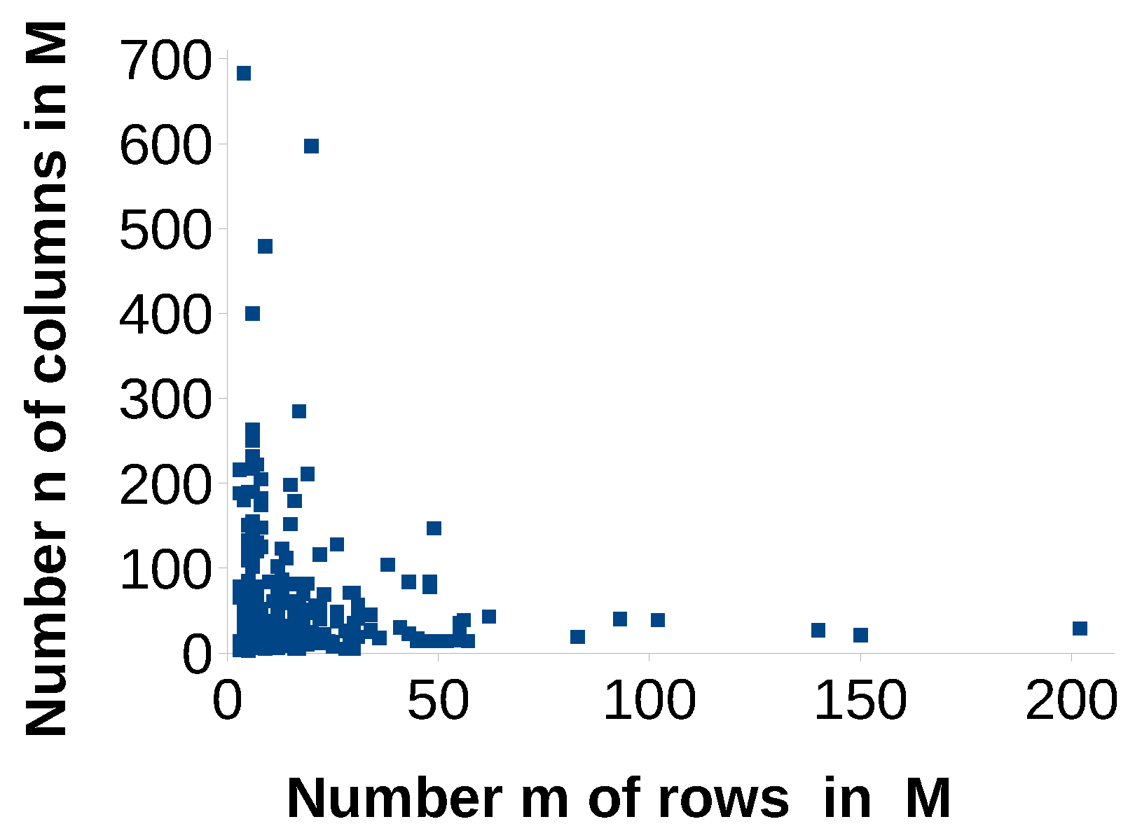
The discrepancy of Brualdi and Sanderson for a given a matrix M (the column and row sums are non-increasing) can range between the minimum and maximum discrepancy in $I_M.$ The current value depends on a “random order of data”, and their corresponding order of columns and row in a matrix. To avoid this variance, we introduced the isomorphic metric $Id\left(M\right)$ that corresponds to the minimum discrepancy in $I_M.$ We want to find out how much this problem really matters in real world matrices. The question is, if the discrepancy value for one single data set (corresponding to a bipartite graph), can change the general statement of how strongly a bipartite network is nested (how small is the discrepancy) completely, or, if the range of possible values is very small, and hence the “order of columns and rows” is negligible. Answering this question, we consider a benchmark data set in ecology of Atmar and Patterson [18]. They offered the first software for several nestedness metrics, and tested it on 291 occurrence matrices representing the absence or presence of animals (mammals, insects, birds) on islands or areas in several regions of the world. These matrices range between dimension 12 ($3\times 4$-matrix), and dimension 11940 ($20\times 597$-matrix). A complete overview of the matrix dimensions is given in Figure 2. In addition, 289 bipartite matrices from them can still be downloaded [19]. (The authors mention in their paper a data set consisting of 294 matrices. The data set we found contains only 291 of their matrices. Two of them (Artreeff.txt und Bajapo.txt) were not complete.) Each of the data text files contains, besides the occurrence matrix, a citation of the paper where the original data set comes from.

3.1. Experiment: Possible Range of Discrepancy in One Isomorphic Class

A matrix M in $I_M$ can possess discrepancy values between $Id\left(M\right)$ (recall that the isomorphic discrepancy is the minimum discrepancy in $I_M$), and maximum discrepancy ${max}_{B\in I_M}\left\{disc\left(B\right)\right\}$ in $I_M.$ A matrix M with a ’random order’ of the rows and columns (without violating the non-increasing order of row and column sums) can have a discrepancy in this range. We determine the discrepancy difference

$$D\left(M\right)=\underset{B\in I_M}{max}\left\{disc\left(B\right)\right\}-Id\left(M\right),$$

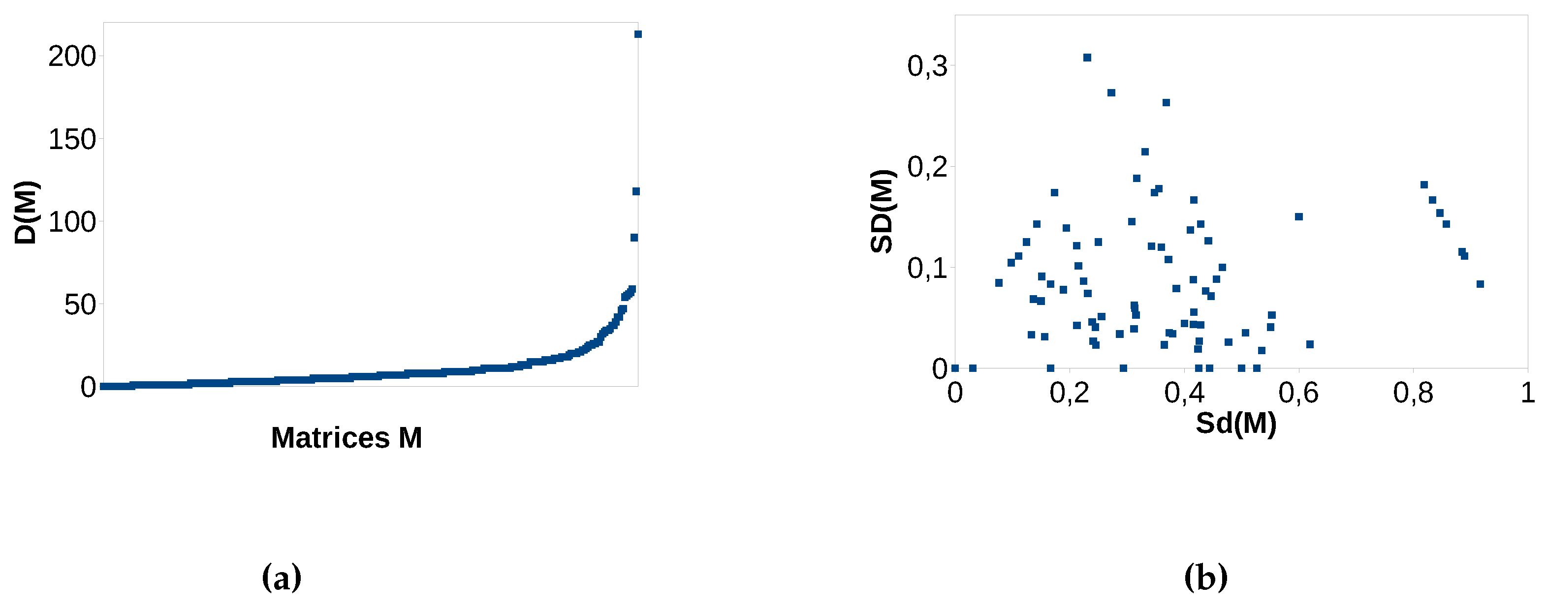
which shows the possible range of the discrepancy value in $I_M.$ Hence, the order of the columns and rows in a matrix can change the discrepancy (nestedness) by the value of the discrepancy difference. The maximum discrepancy ${max}_{B\in I_M}\left\{disc\left(B\right)\right\}$ can be calculated analogously to the determination of $Id\left(M\right)$ with the difference, that we calculate maximum and not minimum weighted perfect matchings. In Figure 3a, one observes for all 289 matrices $M,$ in Atmars and Pattersons benchmark, the values $D\left(M\right).$ Furthermore, we want to see if we find a dependency between the number of 1 s in matrix $M,$ and its difference value $M.$

We observe that the discrepancy difference, i.e., the overestimation (underestimation) of the discrepancy (nestedness), can range between 0 and 220 for a matrix $M.$ Most values lay between 0 and $70.$ However, it is difficult to decide how strong this overestimation really is in considering absolute values. We decided to standardize the discrepancy to get an impression of how strong it is overestimated.

3.2. Experiment: Standardized Discrepancy Difference

For a standardization of the discrepancy $disc\left(M\right)$ of a matrix M, we determined a matrix B with maximum discrepancy in the set $\mathcal{R}$ of all matrices with same row sums. The idea behind this standardization is the following. All matrices in $\mathcal{R}$ possess the same Ferrers matrix $F.$ We look for a matrix B in which a maximum number of 1 s needs to be shifted to achieve F (maximum discrepancy). The standardized discrepancies of M is defined by $Sd\left(M\right)=disc\left(M\right)/disc\left(B\right).$ The algorithm to determine B was given by Brualdi and Sanderson [17] (Section 3). Notice, that the Ferrers matrix F in $\mathcal{R}$ has discrepancy $0.$ Hence, $Sd\left(F\right)=disc\left(F\right)/disc\left(B\right)=0,$ $Sd\left(B\right)=1,$ and all other discrepancies of $\mathcal{R}$ lay between 0 and $1.$

Following the idea in Section 3.1 we want to find out the range of a standardized discrepancy for each matrix M in $I_M.$ We determined the standardized discrepancy difference

$$SD\left(M\right):=\frac{D\left(M\right)}{disc\left(B\right)}$$

for all 289 occurrence matrices in Atmar and Patterson’s data set (see Section 3.1) (consider Figure 3b). We observe (y-axis) that the value of standardized discrepancy difference $SD\left(M\right)$ lays between 0 and $0.3$ for the whole data set. Its size is not dependent on the standardized discrepancy $Sd\left(M\right)$ of M (x-axis). However, it happens that a matrix M with high nestedness (low discrepancy) ($Sd\left(M\right)=0.25$) in the data set could be evaluated as “not so much nested” ($Sd\left(M^{\prime }\right)=0.55$, $M^{\prime }\in I_M$) only because the columns and rows of $M^{\prime }$ occur in another order than in $M.$ For many matrices, the difference is not too high, but still changes the strength of nestedness (standardized discrepancy) by about 10–20%. Some very low nested matrices M ($Sd\left(M\right)$ between $0.8$ and $0.9$) can be evaluated as completely un-nested ($Sd\left(M^{\prime }\right)=1$) with a worst case ordering $M^{\prime }$ of its columns.

4. Conclusions

In summary, it turns out that it is worth considering the isomorphic discrepancy instead of the discrepancy. The isomorphic discrepancy is invariant against a “random order” of columns and rows in a bi-adjacency matrix representing a bipartite graph, and determines a unique value for nestedness. Furthermore, it can be reproduced by every scientist. Moreover, our experiments with occurrence matrices from ecology show that the strength of nestedness can be underestimated by 10–20%. Considering the standardized discrepancy values, Figure 3b shows that standardized discrepancy values are often not larger than $0.5,$ i.e., the nestedness is mostly high or of middle size but very rarely small. A worst case scenario, in which all these matrices are sorted such that the discrepancy is maximised, gave us a standardized discrepancy which ranges between 0 and $0.82$ More precisely, 68 matrices out of 289, with an optimal ordering in matrix M have $disc\left(M\right)=Id\left(M\right)<0.5$ (weakly until middle nested), and if the same matrices have a worst case ordering in matrix $M^{\prime }$, we find $disc\left(M^{\prime }\right)\ge 0.5$ (middle until strongly nested). Those confusing results can be avoided by using the new metric.

References

- Hultén, E. Outline of the History of Arctic and Boreal Biota During the Quaternary Periods; AICS Research, Inc.: Stockholm, Sweden, 1937. [Google Scholar]
- Ulrich, W.; Almeida-Neto, M.; Gotelli, N.J. A consumer’s guide to nestedness analysis. Oikos 2009, 118, 3–17. [Google Scholar] [CrossRef]
- Bascompte, J.; Jordano, P.; Melián, C.J.; Olesen, J.M. The nested assembly of plant-animal mutualistic networks. Proc. Natl. Acad. Sci. USA 2003, 100, 9383–9387. [Google Scholar] [CrossRef] [PubMed]
- Okuyama, T.; Holland, J.N. Network structural properties mediate the stability of mutualistic communities. Ecol. Lett. 2008, 11, 208–216. [Google Scholar] [CrossRef] [PubMed]
- Bastolla, U.; Fortuna, M.A.; Pascual-Garcia, A.; Ferrera, A.; Luque, B.; Bascompte, J. The architecture of mutualistic networks minimizes competition and increases biodiversity. Nature 2009, 458, 1018–1020. [Google Scholar] [CrossRef] [PubMed]
- Thébault, E.; Fontaine, C. Stability of Ecological Communities and the Architecture of Mutualistic and Trophic Networks. Science 2010, 329, 853–856. [Google Scholar] [CrossRef] [PubMed]
- Sylvester, J.J.; Franklin, F. A Constructive Theory of Partitions, Arranged in Three Acts, an Interact and an Exodion. Am. J. Math. 1882, 5, 251–330. [Google Scholar] [CrossRef]
- Ryser, H.J. Combinatorial Properties of Matrices of Zeros and Ones. In Classic Papers in Combinatorics; Gessel, I., Rota, G.C., Eds.; Birkhäuser Boston: Bosten, MA, USA, 1987; pp. 269–275. [Google Scholar]
- Brualdi, R.A. Combinatorial Matrix Classes; Cambridge University Press: Cambridge, UK, 2006. [Google Scholar]
- Mahadev, N.V.R.; Peled, U.N. Threshold Graphs and Related Topics; North-Holland: Amsterdam, The Netherlands, 1995. [Google Scholar]
- Brualdi, R.A.; Shen, J. Discrepancy of matrices of zeros ond ones. Electron. J. Comb. 1999, 6, 1–12. [Google Scholar]
- Lovász, L.; Plummer, M.D. Matching Theory; AMS Chelsea Publishing: New York, NY, USA, 2009; Volume 367. [Google Scholar]
- Gabow, H. Implementation of Algorithms for Maximum Matching on Nonbipartite Graph. Ph.D. Thesis, Stanford University, Stanford, CA, USA, 1974. [Google Scholar]
- Yannakakis, M. Computing the Minimum Fill-In is NP-Complete. SIAM J. Algebraic Discret. Methods 1981, 2, 77–79. [Google Scholar] [CrossRef]
- Garey, M.R.; Johnson, D.S. Computers and Intractability; A Guide to the Theory of NP-Completeness; W. H. Freeman & Co.: New York, NY, USA, 1990. [Google Scholar]
- Junttila, E. Patterns in permuted binary matrices. Ph.D. Thesis, University of Helsinki, Helsinki, Finland, 2011. [Google Scholar]
- Brualdi, A.R.; Sanderson, G.J. Nested species subsets, gaps, and discrepancy. Oecologia 1998, 119, 256–264. [Google Scholar] [CrossRef] [PubMed]
- Atmar, W.; Patterson, B.D. The Nestedness Temperature Calculator: A Visual Basic Program, Including 294 Presence-Absence Matrices; AICS Research, Inc.: Chicago, IL, USA, 1995. [Google Scholar]
- Nested. Available online: https://www.dropbox.com/sh/jbi3bgsalw6e6kt/AAAyDRth-1knfjhYwRqAgqEya?dl=0 (accessed on 23 June 2017).
Figure 1.
A bipartite graph and its bi-adjacency matrix Matrix N is nested because each bee pollinates the same plants as all bees which pollinate more or an equal number of plants.
Figure 2.
Dimensions of 289 occurence matrices in Atmar and Patterson’s benchmark data.
Figure 3.
(a) each data point is a matrix M (x-axis) versus discrepancy difference (y-axis); (b) standardized discrepancy (x-axis) versus standardized discrepancy difference (y-axis).
© 2017 by the authors. Licensee MDPI, Basel, Switzerland. This article is an open access article distributed under the terms and conditions of the Creative Commons Attribution (CC BY) license (http://creativecommons.org/licenses/by/4.0/).
Share and Cite
MDPI and ACS Style
Berger, A.; Schreck, B. The Isomorphic Version of Brualdi’s and Sanderson’s Nestedness. Algorithms 2017, 10, 74. https://doi.org/10.3390/a10030074
AMA Style
Berger A, Schreck B. The Isomorphic Version of Brualdi’s and Sanderson’s Nestedness. Algorithms. 2017; 10(3):74. https://doi.org/10.3390/a10030074
Chicago/Turabian StyleBerger, Annabell, and Berit Schreck. 2017. "The Isomorphic Version of Brualdi’s and Sanderson’s Nestedness" Algorithms 10, no. 3: 74. https://doi.org/10.3390/a10030074
Note that from the first issue of 2016, this journal uses article numbers instead of page numbers. See further details here.