
Engineering a Combinatorial Laplacian Solver: Lessons Learned †

Abstract
:1. Introduction
1.1. Related Work
1.2. Motivation, Outline and Contribution
2. Preliminaries
2.1. Fundamentals
2.2. Cycles, Spanning Trees and Stretch
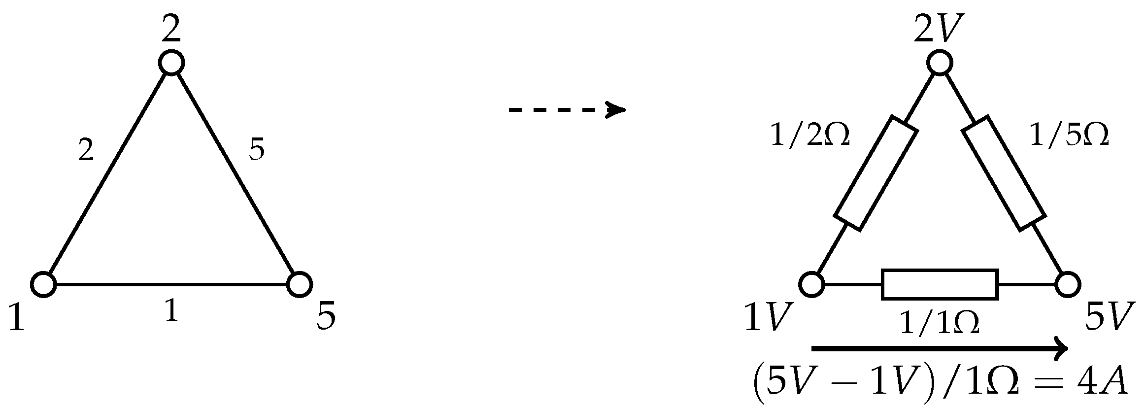
2.3. Electrical Network Analogy
2.4. KOSZ (Simple) Solver
| Algorithm 1: inv-laplacian-current solver KOSZ. |
 |
3. Implementation
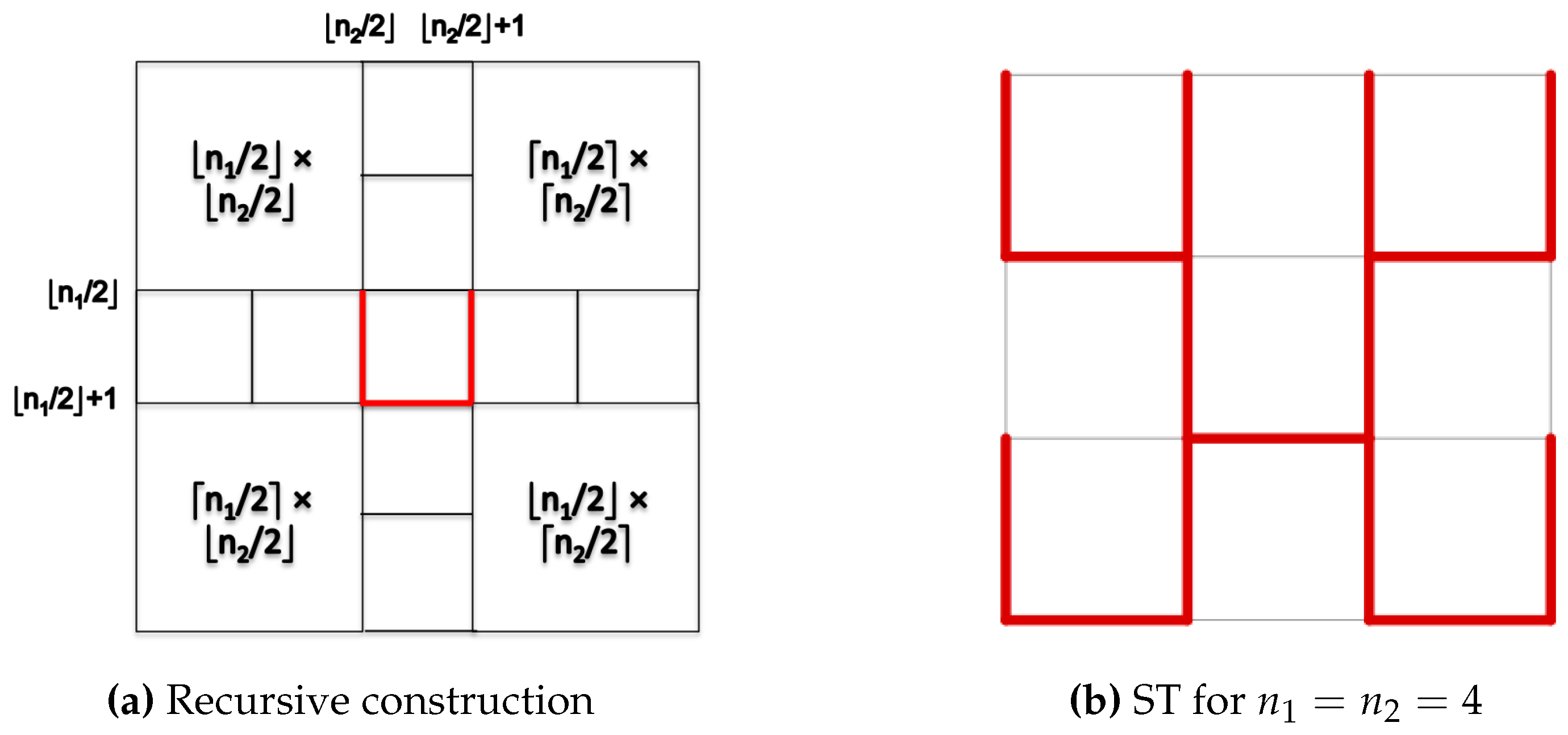
3.1. Spanning Trees
3.2. Flows on Trees


3.3. Linear Time Updates
3.4. Logarithmic Time Updates
3.5. Results
3.6. Remarks on Initial Solution and Cycle Selection
3.7. Summary
4. Evaluation
4.1. Settings
4.1.1. Software, Hardware and Data
4.1.2. Termination and Performance Counters
4.2. Results
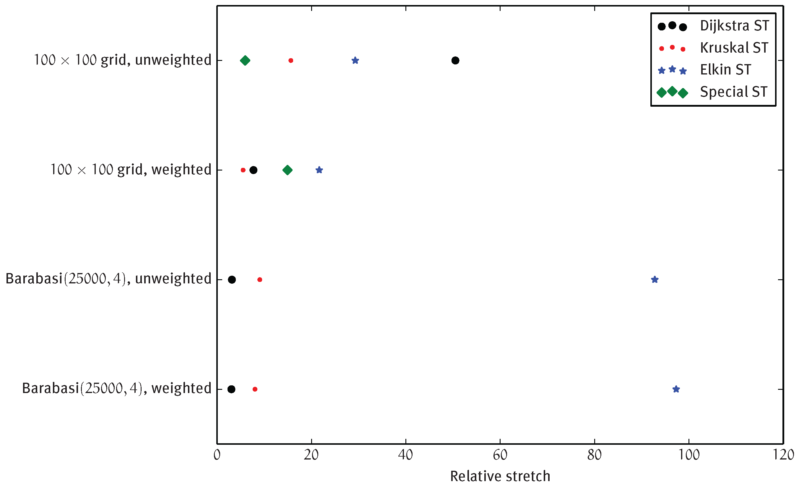
4.2.1. Spanning Tree
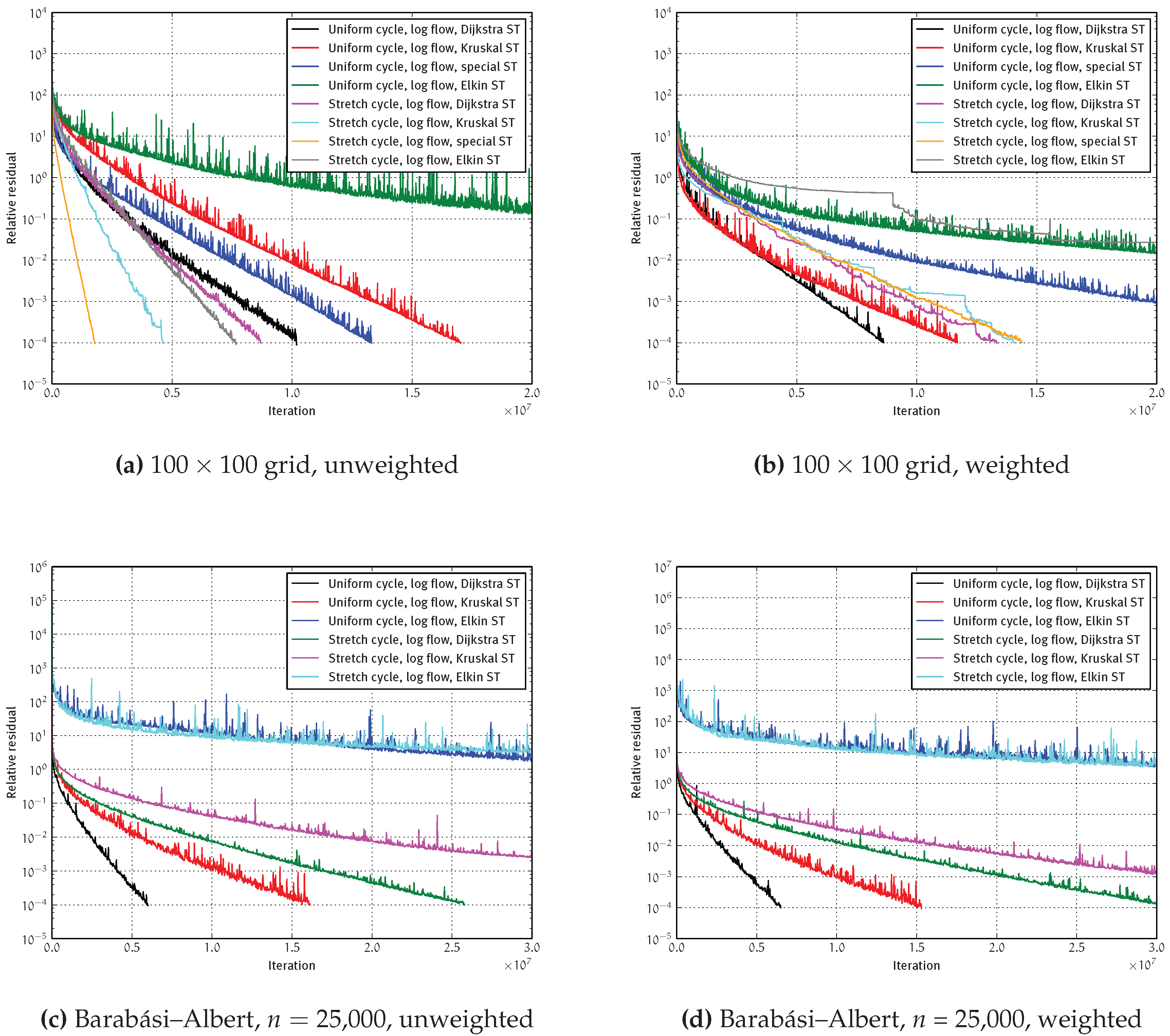
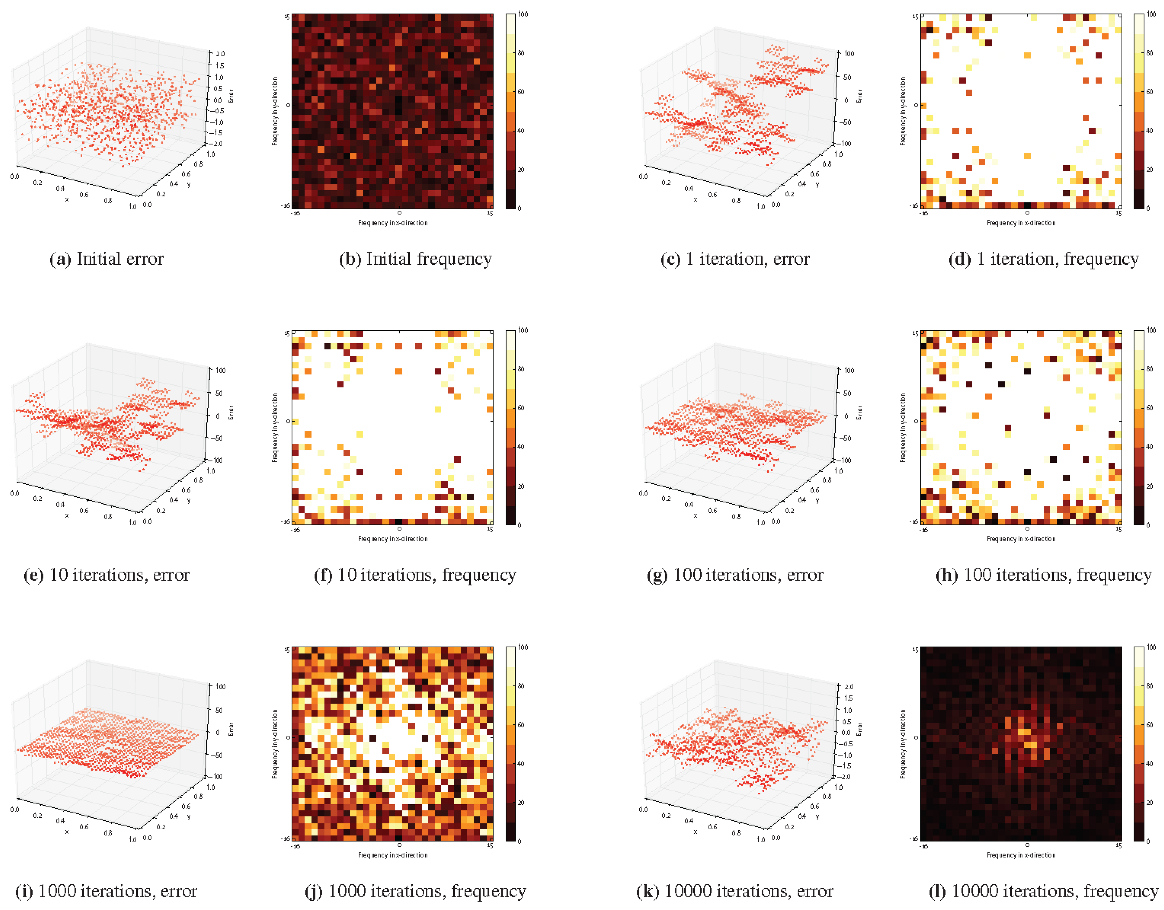
4.2.2. Convergence
4.2.3. Asymptotics
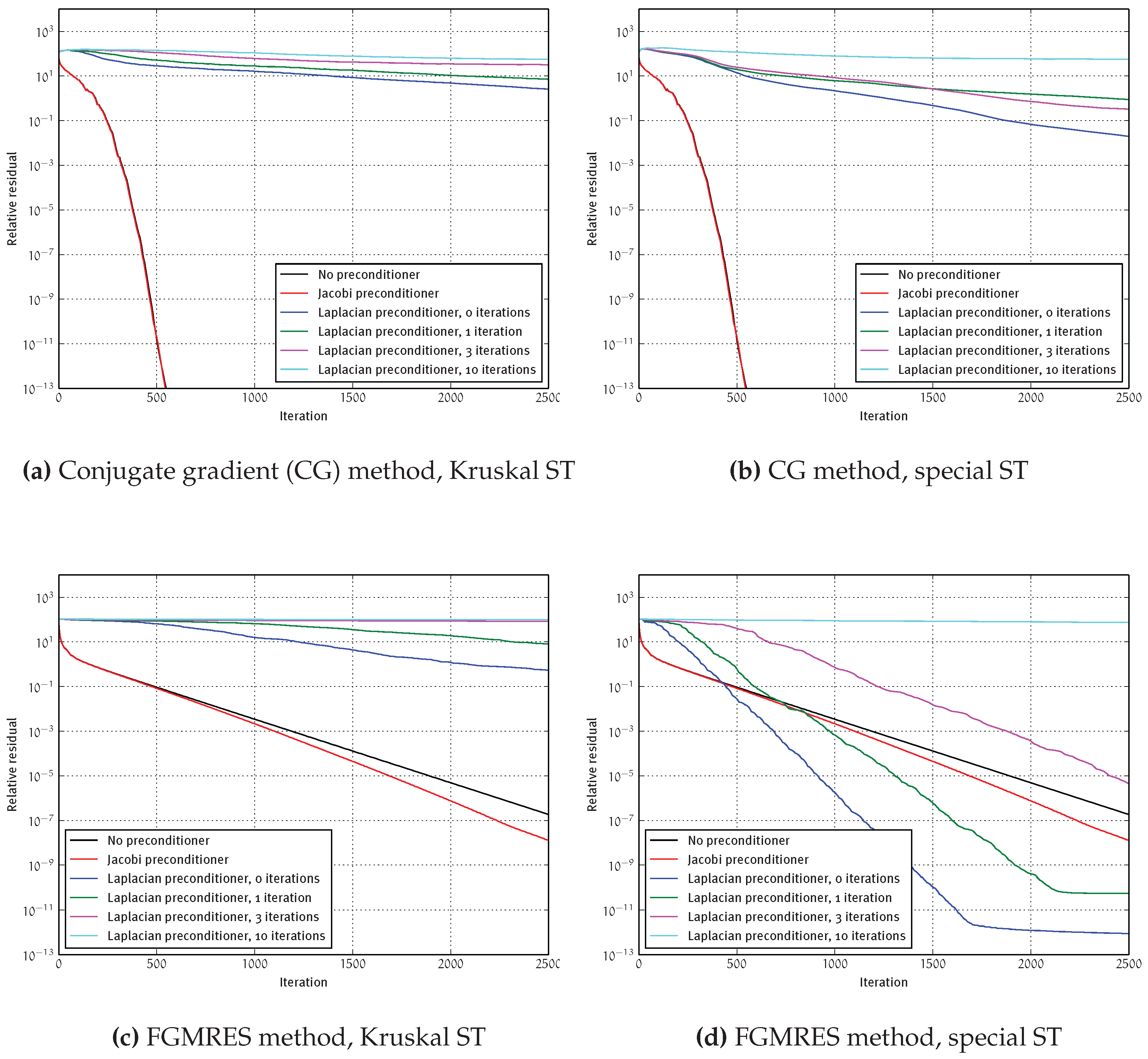
4.2.4. Preconditioning
4.2.5. Smoothing
4.2.6. Cache Behavior
5. Conclusions
Acknowledgments
Author Contributions
Conflicts of Interest
References
- Jasak, H. OpenFOAM: Open source CFD in research and industry. Int. J. Nav. Archit. Ocean Eng. 2009, 1, 89–94. [Google Scholar]
- Spielman, D.A.; Teng, S. Nearly-linear time algorithms for graph partitioning, graph sparsification, and solving linear systems. In Proceedings of the 36th Annual ACM Symposium on Theory of Computing (STOC), Chicago, IL, USA, 13–16 June 2004; pp. 81–90.
- Vaidya, P.M. Solving Linear Equations with Symmetric Diagonally Dominant Matrices by Constructing Good Preconditioners; Technical Report; University of Illinois at Urbana-Champaign: Urbana, IL, USA, 1990. [Google Scholar]
- Boman, E.; Hendrickson, B.; Vavasis, S. Solving Elliptic Finite Element Systems in Near-Linear Time with Support Preconditioners. SIAM J. Numer. Anal. 2008, 46, 3264–3284. [Google Scholar] [CrossRef]
- Christiano, P.; Kelner, J.A.; Madry, A.; Spielman, D.A.; Teng, S.H. Electrical Flows, Laplacian Systems, and Faster Approximation of Maximum Flow in Undirected Graphs. In Proceedings of the 43rd ACM Symposium on Theory of Computing (STOC), San Jose, CA, USA, 6–8 June 2011; pp. 273–282.
- Meyerhenke, H.; Nöllenburg, M.; Schulz, C. Drawing Large Graphs by Multilevel Maxent-Stress Optimization. In Graph Drawing and Network Visualization—23rd International Symposium, GD 2015, Revised Selected Papers; Springer: Berlin/Heidelberg, Germany, 2015; Volume 9411, pp. 30–43. [Google Scholar]
- Spielman, D.A.; Srivastava, N. Graph Sparsification by Effective Resistances. SIAM J. Comput. 2011, 40, 1913–1926. [Google Scholar] [CrossRef]
- Kelner, J.A.; Madry, A. Faster Generation of Random Spanning Trees. In Proceedings of the 50th Annual IEEE Symposium on Foundations of Computer Science (FOCS), Los Alamitos, CA, USA, 2009; pp. 13–21.
- Diekmann, R.; Frommer, A.; Monien, B. Efficient schemes for nearest neighbor load balancing. Parallel Comput. 1999, 25, 789–812. [Google Scholar] [CrossRef]
- Meyerhenke, H.; Schamberger, S. A Parallel Shape Optimizing Load Balancer. In Proceedings of the 12th International Euro-Par Conference (Euro-Par 2006), Dresden, Germany, 28 August–1 September 2006; pp. 232–242.
- Grady, L.; Schwartz, E.L. Isoperimetric graph partitioning for image segmentation. IEEE Trans. Pattern Anal. Mach. Intell. 2006, 28, 469–475. [Google Scholar] [CrossRef] [PubMed]
- Kelner, J.A.; Orecchia, L.; Sidford, A.; Zhu, Z.A. A Simple, Combinatorial Algorithm for Solving SDD Systems in Nearly-linear Time. In Proceedings of the Forty-Fifth Annual ACM Symposium on Theory of Computing, Palo Alto, CA, USA, 1–4 June 2013; pp. 911–920.
- Reif, J. Efficient approximate solution of sparse linear systems. Comput. Math. Appl. 1998, 36, 37–58. [Google Scholar] [CrossRef]
- Spielman, D.A.; Woo, J. A Note on Preconditioning by Low-Stretch Spanning Trees. 2009. Available online: https://arxiv.org/abs/0903.2816 (accessed on 25 October 2016).
- Koutis, I.; Levin, A.; Peng, R. Improved spectral sparsification and numerical algorithms for SDD matrices. In Proceedings of the 29th Symposium on Theoretical Aspects of Computer Science (STACS), Paris, France, 29 February–3 March 2012; pp. 266–277.
- Koutis, I.; Miller, G.L.; Peng, R. Approaching Optimality for Solving SDD Linear Systems. SIAM J. Comput. 2014, 43, 337–354. [Google Scholar] [CrossRef]
- Spielman, D.A. Laplacian Linear Equations, Graph Sparsification, Local Clustering, Low-Stretch Trees, etc. Available online: https://sites.google.com/a/yale.edu/laplacian/ (accessed on 26 October 2016).
- Peng, R.; Spielman, D.A. An Efficient Parallel Solver for SDD Linear Systems. In Proceedings of the 46th Annual ACM Symposium on Theory of Computing, New York, NY, USA, 31 May–3 June 2014; pp. 333–342.
- Koutis, I. Simple parallel and distributed algorithms for spectral graph sparsification. In Proceedings of the 26th ACM Symposium on Parallelism in Algorithms and Architectures (SPAA), Prague, Czech Republic, 23–25 June 2014; pp. 61–66.
- Alon, N.; Karp, R.M.; Peleg, D.; West, D. A Graph-Theoretic Game and its Application to the k-Server Problem. SIAM J. Comput. 1995, 24, 78–100. [Google Scholar] [CrossRef]
- Elkin, M.; Emek, Y.; Spielman, D.A.; Teng, S.H. Lower-stretch Spanning Trees. In Proceedings of the 37th Annual ACM Symposium on Theory of Computing (STOC), Baltimore, MD, USA, 22–24 May 2005; pp. 494–503.
- Abraham, I.; Bartal, Y.; Neiman, O. Nearly Tight Low Stretch Spanning Trees. In Proceedings of the 49th Annual Symposium on Foundations of Computer Science, Philadelphia, PA, USA, 26–28 October 2008; pp. 781–790.
- Abraham, I.; Neiman, O. Using Petal-decompositions to Build a Low Stretch Spanning Tree. In Proceedings of the 44th ACM Symposium on Theory of Computing, New York, NY, USA, 20–22 May 2012; pp. 395–406.
- Papp, P.A. Low-Stretch Spanning Trees. Bachelor Thesis, Eötvös Loránd University, Budapest, Hungary, 2014. Available online: http://www.cs.elte.hu/blobs/diplomamunkak/bsc_alkmat/2014/papp_pal_andras.pdf (accessed on 25 October 2016). [Google Scholar]
- Koutis, I.; Miller, G.L.; Tolliver, D. Combinatorial Preconditioners and Multilevel Solvers for Problems in Computer Vision and Image Processing. Comput. Vis. Image Underst. 2011, 115, 1638–1646. [Google Scholar] [CrossRef]
- Livne, O.E.; Brandt, A. Lean algebraic multigrid (LAMG): Fast Graph Laplacian Linear Solver. SIAM J. Sci. Comput. 2012, 34, B499–B522. [Google Scholar] [CrossRef]
- Dell’Acqua, P.; Frangioni, A.; Serra-Capizzano, S. Accelerated multigrid for graph Laplacian operators. Appl. Math. Comput. 2015, 270, 193–215. [Google Scholar] [CrossRef]
- Dell’Acqua, P.; Frangioni, A.; Serra-Capizzano, S. Computational evaluation of multi-iterative approaches for solving graph-structured large linear systems. Calcolo 2015, 52, 425–444. [Google Scholar] [CrossRef]
- Boman, E.G.; Deweese, K.; Gilbert, J.R. Evaluating the Dual Randomized Kaczmarz Laplacian Linear Solver. Informatica 2016, 40, 95–107. [Google Scholar]
- Hoske, D.; Lukarski, D.; Meyerhenke, H.; Wegner, M. Is Nearly-Linear the Same in Theory and Practice? A Case Study with a Combinatorial Laplacian Solver. In Proceedings of the 14th International Symposium on Experimental Algorithms (SEA 2015), Paris, France, 29 June–1 July 2015; pp. 205–218.
- Harel, D.; Tarjan, R.E. Fast Algorithms for Finding Nearest Common Ancestors. SIAM J. Comput. 1984, 13, 338–355. [Google Scholar] [CrossRef]
- Bender, M.A.; Farach-Colton, M. The LCA Problem Revisited. In LATIN 2000: Theoretical Informatics; Springer: Berlin/Heidelberg, Germany, 2000; Volume 1776, pp. 88–94. [Google Scholar]
- Sleator, D.D.; Tarjan, R.E. A data structure for dynamic trees. J. Comput. Syst. Sci. 1983, 26, 362–391. [Google Scholar] [CrossRef]
- Staudt, C.L.; Sazonovs, A.; Meyerhenke, H. NetworKit: A Tool Suite for Large-scale Complex Network Analysis. Netw. Sci. 2016. accepted. [Google Scholar]
- Hoske, D.; Lukarski, D.; Meyerhenke, H.; Wegner, M. Implementation of KOSZ solver. code: Available online: https://algohub.iti.kit.edu/parco/NetworKit/NetworKit-SDD (accessed on 25 October 2016).
- Guennebaud, G.; Jacob, B. Eigen v3. 2011. Available online: http://eigen.tuxfamily.org (accessed on 25 October 2016).
- Lukarski, D. Paralution—Library for Iterative Sparse Methods. 2015. Available online: http://www.paralution.com (accessed on 20 November 2015).
- Barabási, A.L.; Albert, R. Emergence of Scaling in Random Networks. Science 1999, 286, 509–512. [Google Scholar] [PubMed]
- Browne, S.; Dongarra, J.; Garner, N.; Ho, G.; Mucci, P. A Portable Programming Interface for Performance Evaluation on Modern Processors. Int. J. High Perform. Comput. Appl. 2000, 14, 189–204. [Google Scholar] [CrossRef]
- Demmel, J.W. Applied Numerical Linear Algebra; Society for Industrial and Applied Mathematics: Philadelphia, PA, USA, 1997. [Google Scholar]
- Marquardt, D. An Algorithm for Least-Squares Estimation of Nonlinear Parameters. J. Soc. Ind. Appl. Math. 1963, 11, 431–441. [Google Scholar] [CrossRef]
- Saad, Y. Iterative Methods for Sparse Linear Systems, 2nd ed.; SIAM: Philadelphia, PA, USA, 2003. [Google Scholar]
- Axelsson, O.; Vassilevski, P. A Black Box Generalized Conjugate Gradient Solver with Inner Iterations and Variable-Step Preconditioning. SIAM J. Matrix Anal. Appl. 1991, 12, 625–644. [Google Scholar] [CrossRef]
- Briggs, W.L.; Henson, V.E.; McCormick, S.F. A Multigrid Tutorial; SIAM: Philadelphia, PA, USA, 2000. [Google Scholar]


| Spanning tree | stretch, time |
| Dijkstra | no stretch bound, time |
| Kruskal | no stretch bound, time |
| Elkin et al. [21] | stretch, time |
| Abraham and Neiman [23] | stretch, time |
| Initialize cycle selection | time |
| Uniform | time |
| Weighted | time |
| Initialize flow | time |
| LCA flow | time |
| Log flow | time |
| Iterations | expected iterations |
| Select a cycle | time |
| Uniform | time |
| Weighted | time |
| Repair cycle | time |
| LCA flow | time |
| Log flow | time |
| Complete solver | expected time |
| Improved solver | expected time |
© 2016 by the authors; licensee MDPI, Basel, Switzerland. This article is an open access article distributed under the terms and conditions of the Creative Commons Attribution (CC-BY) license (http://creativecommons.org/licenses/by/4.0/).
Share and Cite
Hoske, D.; Lukarski, D.; Meyerhenke, H.; Wegner, M. Engineering a Combinatorial Laplacian Solver: Lessons Learned. Algorithms 2016, 9, 72. https://doi.org/10.3390/a9040072
Hoske D, Lukarski D, Meyerhenke H, Wegner M. Engineering a Combinatorial Laplacian Solver: Lessons Learned. Algorithms. 2016; 9(4):72. https://doi.org/10.3390/a9040072
Chicago/Turabian StyleHoske, Daniel, Dimitar Lukarski, Henning Meyerhenke, and Michael Wegner. 2016. "Engineering a Combinatorial Laplacian Solver: Lessons Learned" Algorithms 9, no. 4: 72. https://doi.org/10.3390/a9040072