
A No Reference Image Quality Assessment Metric Based on Visual Perception †

College of Computer Science and Technology, Xi’an University of Science and Technology, Xi’an 710054, China
*
Author to whom correspondence should be addressed.
†
This paper is an extended version of our paper published in the International Symposium on Computer, Consumer and Control, Xi’an, China, 4–6 July 2016.
Algorithms 2016, 9(4), 87; https://doi.org/10.3390/a9040087
Submission received: 30 August 2016
/
Revised: 8 December 2016
/
Accepted: 12 December 2016
/
Published: 16 December 2016
(This article belongs to the Special Issue Selected Papers from 2016 International Symposium on Computer, Consumer and Control (IS3C 2016))
Abstract
:Nowadays, how to evaluate image quality reasonably is a basic and challenging problem. In view of the present no reference evaluation methods, they cannot reflect the human visual perception of image quality accurately. In this paper, we propose an efficient general-purpose no reference image quality assessment (NRIQA) method based on visual perception, and effectively integrates human visual characteristics into the NRIQA fields. First, a novel algorithm for salient region extraction is presented. Two characteristics graphs of texture and edging of the original image are added to the Itti model. Due to the normalized luminance coefficients of natural images obey the generalized Gauss probability distribution, we utilize this characteristic to extract statistical features in the regions of interest (ROI) and regions of non-interest respectively. Then, the extracted features are fused to be an input to establish the support vector regression (SVR) model. Finally, the IQA model obtained by training is used to predict the quality of the image. Experimental results show that this method has good predictive ability, and the evaluation effect is better than existing classical algorithms. Moreover, the predicted results are more consistent with human subjective perception, which can accurately reflect the human visual perception to image quality.
1. Introduction
With the rapid development of information technologies and widespread usage of smart phones, digital imaging has become a more and more important medium to acquire information and communicate with other people. These digital images generally suffer impairments during the process of acquisition, compression, transmission, processing and storage. In addition, these phenomena have brought us great difficulties in studying images and understanding the objective world. Because of this, the image quality assessment (IQA) metrics have become a fundamentally important and challenging work. Effective IQA metrics could play important roles in applications such as dynamic monitoring and adjustment of image quality, optimizing the parameter settings of image processing systems, and searching high quality images of medical imaging and so on [1]. For one thing, high quality images can help doctors to judge the severity of the disease in medical fields. For another, such as high-definition televisions, personal digital assistants, internet video streaming, and video on demand, necessitate the means to evaluate the images quality of this information. Therefore, in order to obtain high quality and high fidelity images, the study of image quality evaluation has important practical significance [2,3].
Because human beings represent terminals for the majority of processed digital images, subjective assessment is the ultimate criterion and reliable image quality assessment method. However, the subjective assessment methods hinder its application in practice because of its disadvantages, such as time-consuming, expensive, complex and laborious. Thus, the goal of objective IQA is to automatically evaluate the quality of images as near to human perception as possible [2].
Based on the availability of a reference image, objective IQA metrics can be classified into full reference (FR), reduced reference (RR), and no reference (NR) approaches [4]. Only recently did FR-IQA methods reach a satisfactory level of performance, as demonstrated by high correlations with human subjective judgments of visual perception. SSIM [5], MS-SSIM [6] and VSNR [7] are examples of successful FR-IQA algorithms. These metrics are based on measuring the similarity between the distorted image and its corresponding original image. However, in real-world applications, where the original is not available, FR metrics are not used. This strictly limits the application domain of FR-IQA algorithms. In addition, the NR-IQA is the only possible algorithm that can be used in the practical application. However, a number of NR-IQA metrics have been testified that they do not always correlate with the perceived image quality [8,9].
Presently, NR-IQA algorithms generally follow one of two trends: The distortion-specific and general-purpose methods. The former evaluate the distorted image of a specific type while the latter directly measure the image quality evaluation without knowing the type of image distortion. Since the result of evaluation ultimately depends on the feeling of the observers, image evaluation with more perfect and more suitable for the actual quality must be based on human visual, psychological characteristics and organic combine the subjective and objective evaluation methods. A large number of studies have shown that: considering the human visual system (HVS) evaluation methods are better than that without considering the characteristics of HVS evaluation methods [10,11,12,13]. However, existing no-reference image quality assessment algorithms are failed to give full consideration to the human visual features [10].
At present, there are some problems in the field of image quality assessment:
- Unable to obtain the original image.
- Difficult to determine whether the type of distortion of the distorted image exists.
- Existing methods lack of considering human visual characteristics.
- How to ensure the characteristics to be not significantly difference caused by the distortion images with same degree yet different types.
In this paper, based on the existing image quality evaluation methods, we draw the human visual attention region mechanism and the HVS characteristics into the no reference image quality assessment method. Then, we propose a universal no-reference image quality assessment method based on visual perception.
The rest of this paper is organized as follows. In Section 2, we describe the current research about no reference image quality assessment methods and visual saliency. In Section 3, we introduce the extraction model of visual region of interest. In Section 4, we provide an overview of the method. In Section 5, we describe blind/reference image spatial quality evaluator (BRISQUE) algorithm and the prediction model is provided in Section 6. We present the results in Section 7, and we conclude in Section 8.
2. Previous Work
Before proceeding, we state some salient aspects of NR-IQA methods. Present day depending on whether we know the type of distortion image or not, NR-IQA methods can be divided into two categories: distortion-specific approaches and general-purpose approaches [14].
Distortion-specific algorithm is capable of assessing the quality of images distorted by a particular distortion type, such as blockiness, ringing, blur after compress, and noise generated during image transmission. In literatures [15,16,17,18], the authors proposed some approaches for JPEG compression images. In [17], Zhou et al. aimed to develop NR-IQA algorithms for JPEG images. At first, they not only established a JPEG image database, but also subjective experiments were conducted on the database. Furthermore, they proposed a computational and memory efficient NR IQA model for JPEG images, and estimated the blockiness by the average differences across block boundaries. They used the average absolute difference between in-block image samples and the zero-crossing rate to estimate the activity of the image signal. At last, subjective experiment results were used to train the model, which achieved good quality prediction performance. For JPEG2000 compression, distortion in an image is generally modeled by measuring edge-spread using an edge-detection based approach and this edge spread is related to quality [5,19,20,21,22]. The literatures [23,24,25] are evaluation algorithms for blur. QingBin Sang et al. calculated image structural similarity by constructing fuzzy counterpart [20]. Firstly, they used a low pass filter to blur the original blurred image and produce re-blurred image. Then they divided the edge dilation image into 8 × 8 blocks. In addition, the sub-blocks were classified into edge dilation block and smooth block. In addition, the gradient structural similarity index was defined by different weighs according to the different types of blocks. Finally, the blur average value of the whole image was produced. The experimental results were shown that the method was more reasonable and stable than others. However, these distortion-specific methods are obviously limited by the fact that it is necessary to know the distortion types in advance, which makes their application field limited [3].
Universal methods are applicable to all distortion types and can be used in any occasion. In recent years, researchers proposed many universal no reference image quality assessment methods. However, most of these methods relied on the prior knowledge of subjective value and distortion types, and used machine learning methods to get the image quality evaluation score. Some meaningful universal methods are reported in the literature [8,26,27,28,29,30,31]. In [26], the author proposed a new two-step framework for no-reference image quality assessment based on natural scene statistics (NSS), namely Blind Image Quality Indices, (BIQI). Firstly, the algorithm estimated the presence of a set of distortions in the image. Secondly, they evaluated the quality of the image according to those distortions. In literature [27], Moorthy et al. proposed a blind IQA method based on the hypothesis that natural scenes have some certain statistical properties. In addition, those properties can make the quality of image degeneration. This algorithm was called Distortion Identification- based Image Verity and Integrity Evaluation (DIIVINE) and also was a two-step framework. The DIIVINE mainly consists of three steps. Firstly, the wavelet coefficients were normalized. Then, they calculated the statistical characteristics of the wavelet coefficients, such as scale and orientation selective statistics, orientation selective statistics, correlations across scales and spatial correlation. Finally, the quality of the image was calculated using those statistical features. The method has achieved a good performance on evaluation. In literature [8], the authors supposed in Discrete Cosine Transform (DCT) domain the change of image statistical characteristics can predict image quality, and proposed Blind Image Integrity Notator using DCT Statistics algorithm (BLIINDS). Subsequently, Saad et al. extended the BLIINDS algorithm, and proposed an alternate approach that relies on a statistical model of local DCT coefficients which they dubbed blind image integrity notator using DCT statistic (BLIINDS-II) [28]. To begin with, they partitioned the image into n × n blocks and computed the local DCT coefficient. Then, they applied a generalized Gaussian density model to each block of DCT coefficients. Furthermore, they computed functions of the derived model parameters. Finally, they used a simple Bayesian model to predict the quality score of the image. In literature [29], Mittal et al. proposed a natural scene statistic-based NR IQA model that operated in the spatial domain, namely blind/reference image spatial quality evaluator (BRISQUE). This method did not compute distortion-specific features, but used scene statistics of locally normalized luminance coefficients to evaluate the quality of the image instead. Since Ruderman found that these normalized luminance values strongly tend towards a unit normal Gaussian characteristic [30] for natural images, this method used this theory to preprocess the image. Then, they extracted features in spatial domain. Those features mainly contain generalized Gauss distribution characteristics and correlation of adjacent coefficients. Finally, those features were used to map the quality to human rating via SVR model. Over the course of last few years, a number of researchers have devoted time to improving the assessment accuracy of NR IQA methods by taking advantage of known natural scene statistics characteristics. These methods are failed to give full consideration to the human visual characteristics [2]. There is also a deviation between the predicted qualities and the real qualities, since the human visual system is the ultimate assessor of image quality. In addition, almost all of the no reference image quality assessment methods are based on gray scale images, and they do not make full use of the color characteristics of the image.
Through above analysis of NR IQA methods, at present, both in distortion-specific and general-purpose methods, almost all of the methods use statistical characteristics of natural images to establish quality evaluation model, and have achieved better effect of evaluation. However, considering the statistical characteristics of natural images can hardly reflect the whole regularities of image quality. There is still a certain gap with the subjective consistency of human vision.
Since the HVS is the ultimate assessor of image quality, a number of image quality assessment methods based on an important feature of the HVS, namely, visual perception, are emerging in the present day [10]. Among them, the research of region of interest (or visual saliency) is a major branch of the HVS. In the field of image processing, ROI of an image are the areas that differ significantly from their adjacent regions. They can immediately attract our eyes and capture our attention. Therefore, the ROI is a very important region in the image quality assessment. On the other hand, how to build a computational visual saliency model has been attracting tremendous attention in recent years [32].
Nowadays, a number of computational models to simulate human visual attention have been studied by scholars and some powerful models have been proposed. For further details of ROI refer to [9,10,11,12,32,33,34,35,36]. In [33], Itti et al. proposed a visual saliency model which was the first influential and best known visual saliency model. In this paper, we call it Itti model. Itti model mainly contains two aspects. Firstly, they introduced image pyramids for feature extraction, which makes the visual saliency computation efficient. Secondly, Itti et al. proposed the biologically inspired “center-surround difference” operation to compute feature dependent saliency maps across scales [32]. This model effectively breaks down the complex problem of scene understanding by rapidly selecting. Following the Itti model, Harel et al. proposed the graph-based visual saliency (GBVS) model [37]. The GBVS was introduced a novel graph-based normalization and combination strategy, and was a new bottom-up visual saliency model. It mainly consists of two steps. The first step is forming activation maps on certain feature channels. In addition, the second step is normalizing them in a way which highlights salient and admits combination with other maps. Experimental results show that the GBVS predicts ROI more reliably than other algorithms.
In this paper, we mainly study the human visual characteristics, extract the region of interest, and combine the statistical characteristics of the natural image as the measurement index of the distortion image. Finally, do experiments on the database LIVE [38], the experimental results show that the features extraction and the learning method are reasonable, and correlate quite well with human perception.
3. Extraction Model of Visual Region of Interest
With the increasingly development of information technology, images have become the main media of information transmission. How to analyze and deal with a large number of image information effectively and accurately is an important subject. Then, researchers have found that the most important information in the image is often focusing on a few key areas. They call these key areas salient regions or regions of interest. We will greatly improve the efficiency and accuracy of image processing and analyzing with extracting these salient regions accurately. So far, there are many regions of interest extraction algorithms. The detection technology of the ROI, which has been based on interaction and detection technology, has gradually developed into based on visual feature technology. The salient map model proposed by Itti is the most typical ROI detection, based on visual features [33]. This method only considers the bottom-up signal, simple and easy to implement. It is the most influential visual attention model.
3.1. The Principle of Itti Model
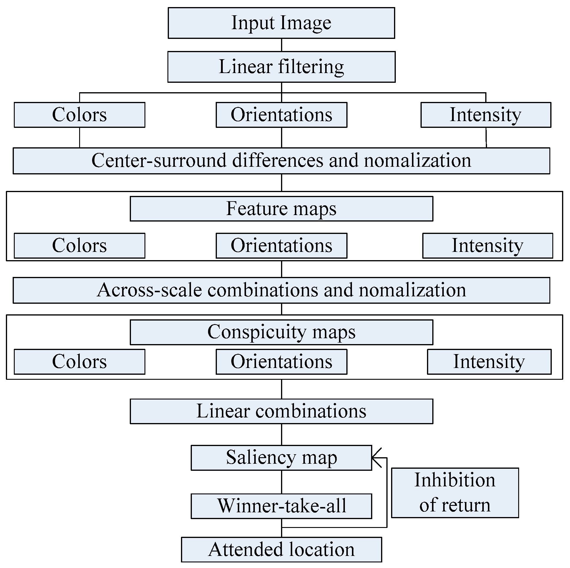
In 1998, Itti et al. proposed an algorithm based on salient map model. The algorithm defines the color, brightness and direction of three kinds of visual characteristics, and uses Gaussian pyramid building scale space. The model uses the center-surround of the compute strategy to form a set of feature maps, and then these collections are normalized and merged to create salient map. It includes three processes of features acquisition, salient map computation, selection and transfer of the region of interest [34,35,36]. Figure 1 is the implementation process of Itti Koch model.
3.2. Algorithm Improvement
In this paper, we propose an improved model based on the idea of Itti model. We add texture feature and edge structure characteristics to the original model. The model block diagram is shown in Figure 2.
3.2.1. Texture Feature Extraction
Texture is an important visual cue, which is a common and difficult feature in the image. The texture feature is consistent with human visual perception process and plays an important role in the region of interest. There are many methods to extract texture features of images currently, such as wavelet extraction methods, gray level co-occurrence matrix (GLCM) extraction methods and so on. In recent years, the wavelet methods have been widely used in many fields. In literatures [39,40], the authors introduced the wavelet method into the medical field and had achieved considerable success. In the former article, the authors used the discrete wavelet packet transform (DWPT) to extract wavelet packet coefficients from MR brain images. In the latter article, to help improve the directional selectivity impaired by discrete wavelet transform, they proposed a dual-tree complex wavelet transform (DTCWT), which was implemented by two separate two-channel filter banks. DTCWT obtained directional selectivity by using approximately analytic wavelets. At each scale of a two dimensions DTCWT, it produces in total six directionally selective sub-bands (±15°, ±45°, ±75°) for both real and imaginary parts. The method can obtain more information about the direction of the images. However, Gabor wavelet is an important method of texture feature extraction. It not only can extract texture features effectively, but also eliminate redundant information. In addition, the frequency and direction of Gabor filter that close to the human visual system for frequency and direction, and they were used for texture representation and description. A series of filtered images can be obtained by convolution of the image with the Gabor filter, and the information of each image on the scale and direction is described in each image [41]. In this paper, we use Gabor wavelet to extract texture features of each filter image. Two dimensional Gabor function g(x, y) can be expressed as:
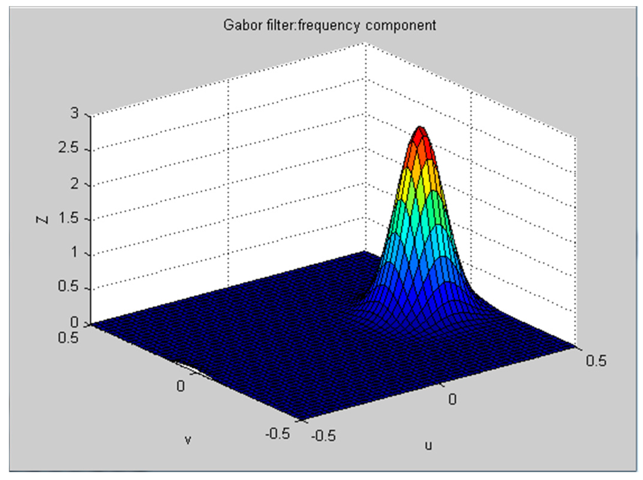
where W is Gaussian function of polyphonic system frequency. According to the accordance with human visual system, W = 0.5. The Fourier transform of g(x, y) can be expressed as:
where , . The frequency spectrum is shown in Figure 3.
In order to get a set of self-similar filters, we use g(x, y) as the generating function, and do moderate scale expansion and rotation transformation on it. That is, Gabor wavelet:
where a > 1, m, n are integer. , , , where θ = nπ/k, and k is the number of direction. m, n are scale and direction respectively, n [0, k]. Figure 4 are four different directions of the Gabor wavelet. Then we use the Gabor wavelet transform to extract the texture features of the image. For an image I(x, y), its Gabor wavelet transform can be defined as:
where, represents the conjugate complex, and the texture features are calculated as shown in Formula (5). In the model, the center-surround is implemented as the difference between fine and coarse scales. The center represent a pixel at scale c {2, 3, 4}, and the surround represent the corresponding pixel at scale s = c + δ, δ {3, 4}. The across-scale difference (denoted “Θ” below) between two maps is acquired by interpolation to the finer scale and point-by-point subtraction.
The above feature maps are combined to get the texture salient map. They are obtained through across-scale addition, “⊕”, which consists of reduction of each map to scale four and point-by-point addition. The combined formula is as follow.
3.2.2. Edge Structure Feature Extraction
Edge is the most important feature of the image. Currently, there are many kinds of edge detection methods, such as Roberts operator detection method, Sobel operator detection method, Prewitt operator detection method and so on. However, because of the noise, the Canny method is not easy to be disturbed, or to detect the real weak edges. The advantage is that the two different thresholds are used to detect strong edges and weak edges. Weak edges are included in the output image when the weak edges and strong edges are connected. In this paper, we use Canny edge detection algorithm to extract the edge structure features of the image. Steps are as follows:
- (1)
- We use Gauss filter to smooth image. Canny method firstly uses two-dimensional Gauss’s function to smooth the image:Its gradient vector is . Where σ is distributed parameter of Gauss filter.
- (2)
- We calculate the magnitude and direction of the gradient, and suppress the amplitude of the gradient.
- (3)
- We perform a dual threshold method to detect and connect edges. E(x, y) is the final edge structure map.
The edge structure characteristic is calculated as:
The above feature maps are combined to get the edge structure salient map. The combined formula is as:
In the end, the final image salient region is obtained by linear addition of 5 salient maps, and the formula is shown below:
where, I, C and O represent intensity, color and orientation feature respectively.
4. Overview of the Method
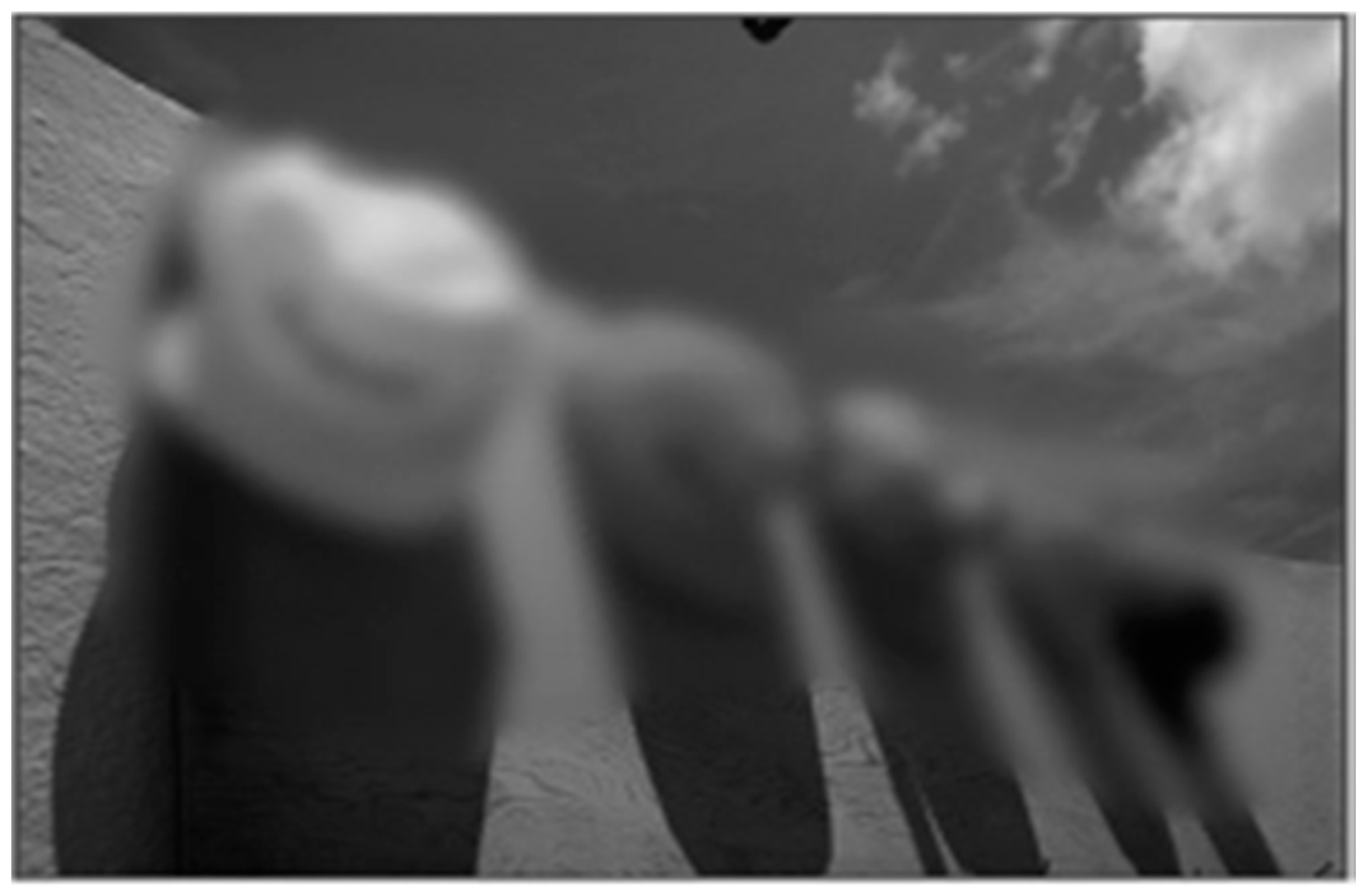
Currently no reference image quality evaluation algorithm can be divided into two categories: distortion-specific methods and universal methods. However, the distortion-specific methods are limited in the practical application because the prior need to determine the type of the distorted images. The general-purpose methods do not depend on the type of distorted images, and have prospect of practical application. However, the existing algorithms are almost to extract natural statistical characteristics of image, and rarely take into account the visual characteristics of the human eye. Thus, in practical application, there is a deviation between the evaluation result and the result of the human eye perception. As shown in Figure 5 and Figure 6, due to the visual characteristics of the human eye, in the same picture, different regions (such as interest and non interest areas) in the same image quality damage degree will make the human eye produce different visual experience. Under the same Gauss fuzzy, the visual observation effect of Figure 5 is better than Figure 6.
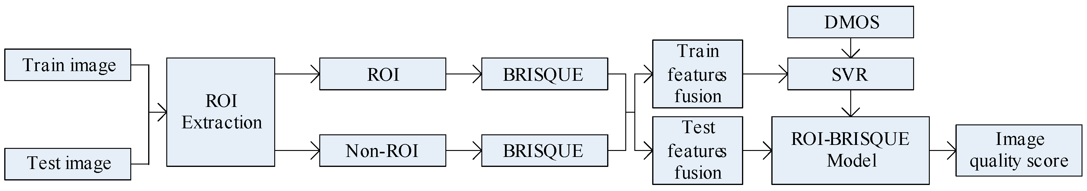
In the observation of the image, human eye will be the first to pay attention to the visual characteristics of the more prominent areas. Although the image suffered the same damage, because of the different regions, the human eye subjective feelings are different. Based on the background, this paper proposes a method of image quality evaluation based on visual perception. Firstly, we extract the region of interest. Secondly, extract the features from the regions of interest and regions of non-interest. Finally, the extracted features are fused effectively, and the image quality evaluation model is established. The proposed approach we called region of interest blind/reference image spatial quality evaluator (ROI-BRISQUE). Figure 7 is the framework of the proposed method in this paper.
The method of this paper is described as follows:
Firstly, the LIVE image database is divided into two categories: training images and testing images. In addition, we extract the region of interest and features on the training images. Then, we use the feature vectors as the input of the ε-SVR, the DMOS of the corresponding image as the output target to train the image quality evaluation model. Finally, the image quality prediction model is used to predict the quality of the distorted image.
This paper focuses on the image region of interest extraction. The traditional Itti model calculates the salient region of the image by extracting the underlying features of the image color, brightness and direction. It can search out the attention region. However, there are still some shortcomings, for instance, the contour of the salient region is not clear. In order to extract the region of interest more accurately, we add texture and edge structure features to the Itti model. Then, we use the improved model to extract the region of interest and region of non-interest, and use BRISQUE algorithm to extract the natural statistical features of the image respectively. Moreover, the characteristics of the region of interest and region of non interest are fused to get the measure factor of the image. We train the image quality evaluation model, which the measure factor as the input and the DMOS value of corresponding image as the output target of SVR. Finally, the quality of the distorted image is predicted by the trained evaluation model.
5. Feature Extraction of BRISQUE Algorithm
Ruderman [30] found that the normalized luminance coefficients of natural images obey the unit generalized Gauss probability distribution. He believes that the image distortion will change the statistical characteristics of the normalized coefficient. By measuring the change of the statistical features, the distortion types can be predicted and the visual quality of the image can be evaluated. Based on this theory, Mittal et al. proposed a BRISQUE algorithm based on spatial statistical features [29]. This spatial method to NR IQA that they have developed can be summarized as follows.
5.1. Image Pixel Normalization
Given an image which possibly distorted, we compute locally normalized luminances via local mean subtraction and divisive normalization. Formula (11) may be applied to a given intensity image I(i, j) to produce:
where I(i, j) represents the gray value of the original image, I ∈ {1,2, …, M}, j ∈ {1,2, ..., N}. M and N are the image height and width respectively; c is a small constant, in order to prevent the stability of calculated results when the denominator closes to 0. μ(i, j) and σ(i, j) are weighted mean and variance. ω = {ωk,l|k = −K, …, K, l = −L, …, L} is a two-dimensional circularly symmetric Gaussian weighting function. They called the normalized brightness value of is MSCN (Mean Subtracted Contrast Normalized) coefficients.
5.2. Spatial Feature Extraction
The existence of distortion will destroy the regularity between the adjacent MSCN coefficients. The characteristics of the normalized coefficients include the generalized Gauss distribution features and the correlation of the adjacent coefficients.
(1) Generalized Gauss distribution characteristics:
The model formula can be expressed as Formula (14).
where , is gamma function. The shape parameter controls the shape of the generalized Gauss model, and σ2 is the variance. This article uses the literature [42] fast matching method to estimate (a, σ2) as the features of generalized Gauss distribution.
(2) Correlation of adjacent coefficients:
We obtain correlation images from the horizontal, vertical, diagonal and diagonal four directions [43], and use Asymmetric Generalized Gaussian Distribution (AGGD) to fit the images. We use fast matching method [44] to estimate parameters (η, ν, σl, σr) for each direction. Thus, we utilize the 16 estimation parameters of four directions as the correlation feature of the adjacent coefficients.
However, due to multiscale statistical characteristics of natural images, the author found that it is much more reasonable to extract two generalized distribution characteristics and 16 neighboring coefficients of correlation characteristics at two scales. Therefore, the total extracted features are (2 + 16) × 2 = 36.
6. Prediction Model
Through being established the relationship between image features and subjective evaluation values of image in this paper, we propose a model of objective image quality evaluation model based on ROI-BRISQUE. We utilize measure factor of distortion image (Vall) which obtained from feature vectors effective fusion between region of interest feature vector (Vroi) and region of non-interest feature vector (Vnon-roi) as the input of the SVR model. Moreover, we use the subjective quality evaluation value of the corresponding image as the output target to establish image quality evaluation model based on visual perception. The calculation formula is given by Formula (15).
The parameter λ is the weight of the image region of interest. Through training on the LIVE image database, the experimental results show that the model has a good learning accuracy and predictive ability.
7. Results and Discussion
7.1. Experimental Results of the Region of Interest
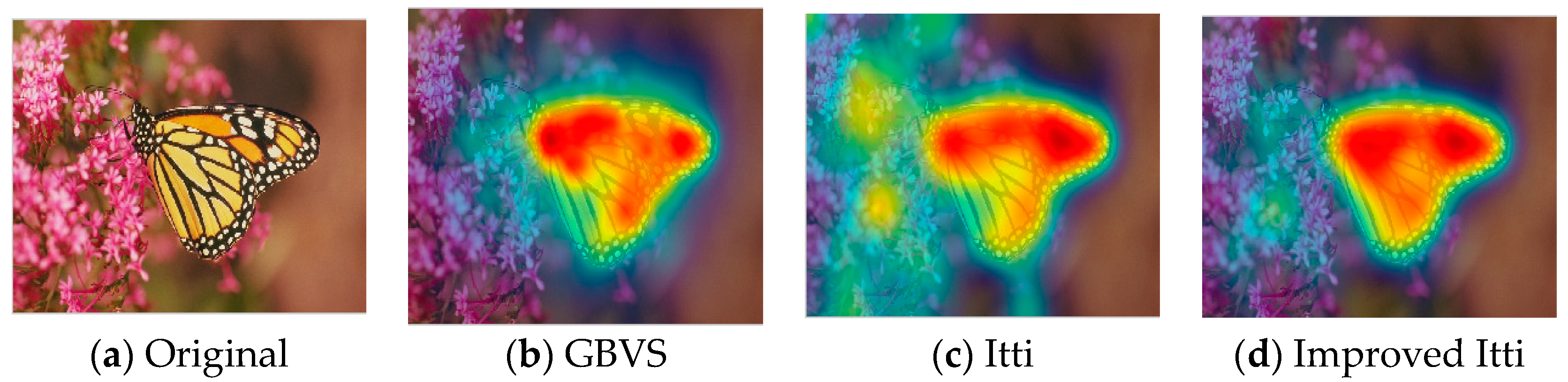
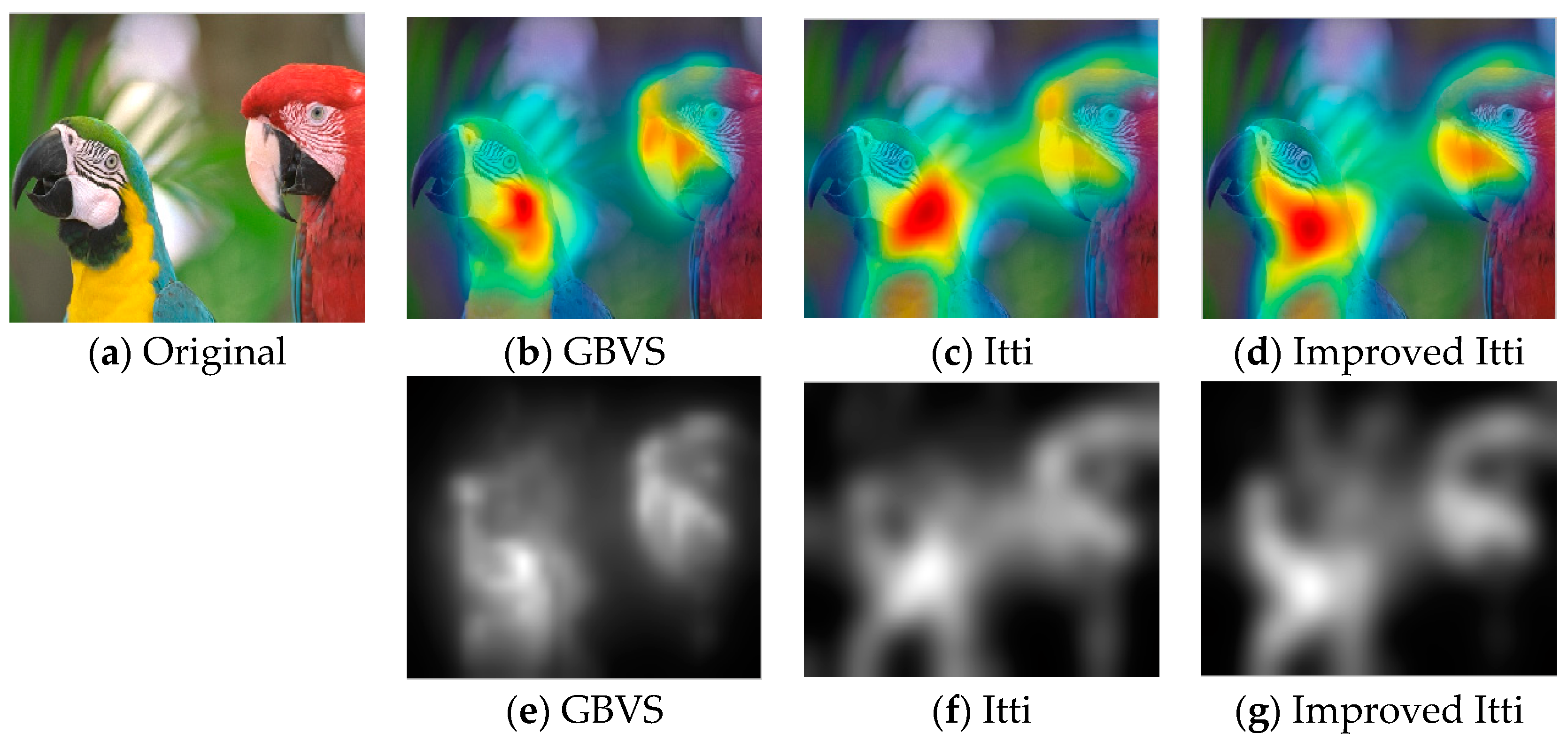
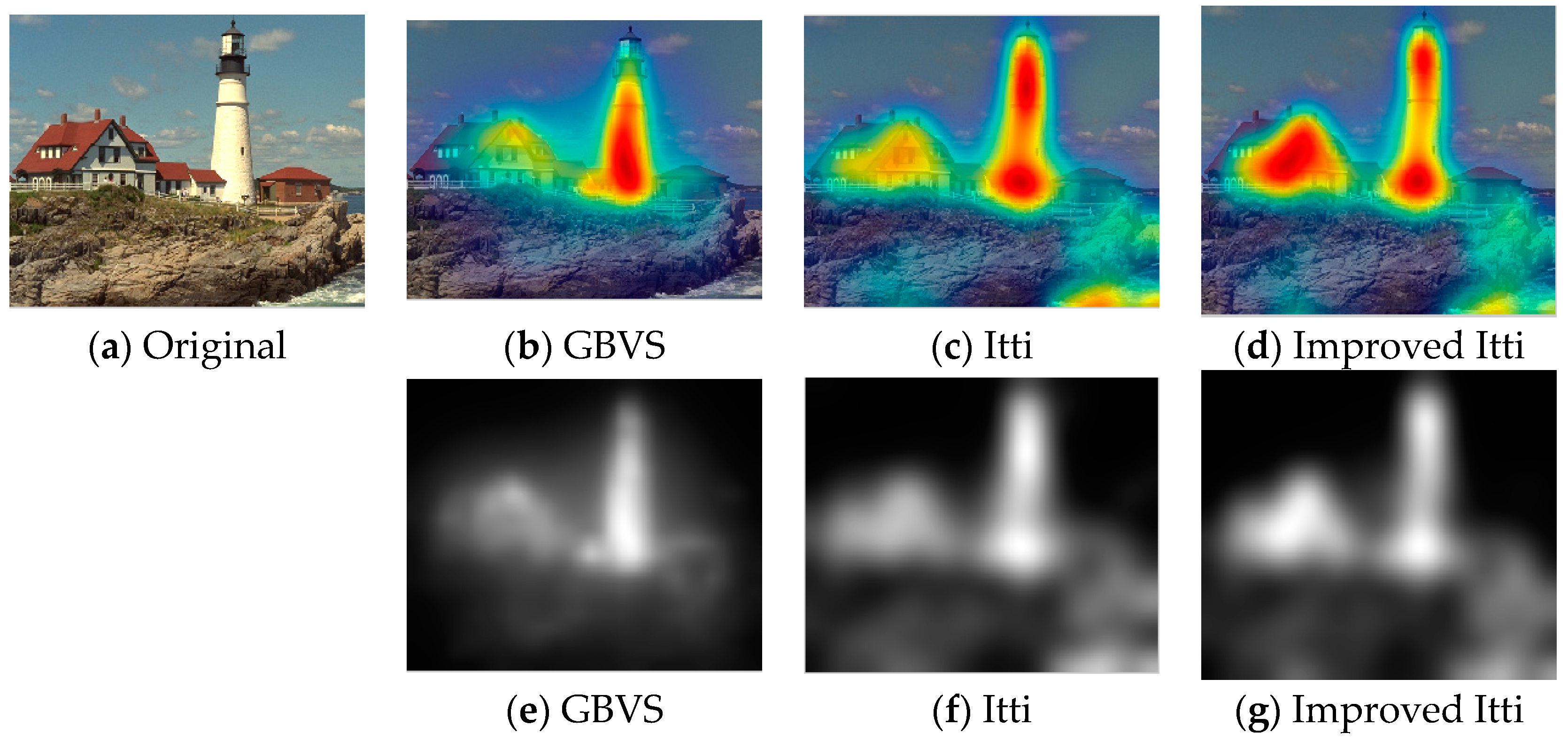
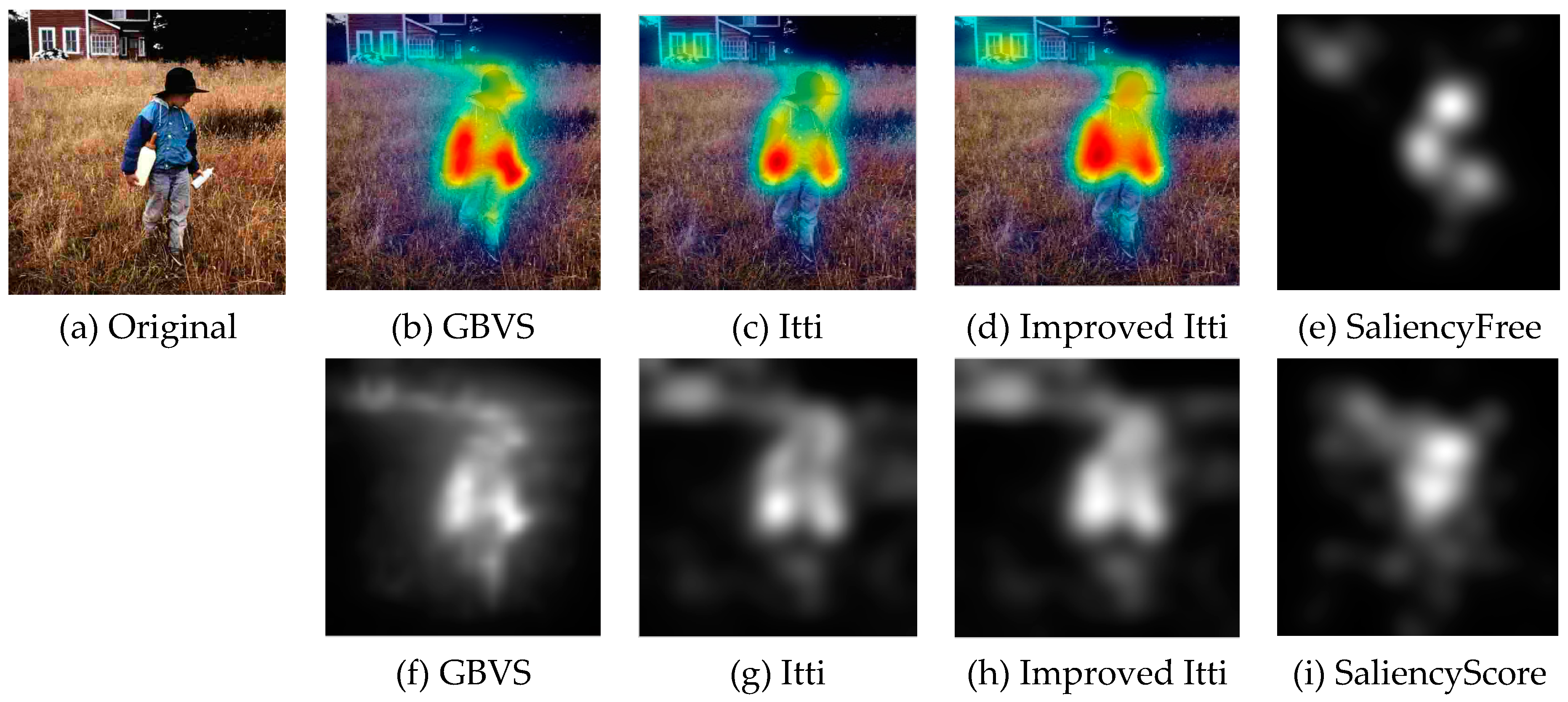
In this paper, we select some pictures from image database to test the improved Itti model. Meanwhile, in order to compare the experimental results, saliency maps of Itti and GBVS are also listed, the results as shown in Figure 8, Figure 9 and Figure 10:
In Figure 8, Figure 9 and Figure 10, (a) is the original image, (b), (c) and (d) are salient overlap maps of Graph-Based Visual Saliency (GBVS) model, Itti model and this paper’s model respectively. (e), (f) and (g) are salient maps of GBVS model, Itti model and this paper’s model respectively. The white areas represent region of interest, and the black areas represent the region of non-interest. The higher the brightness of the white part is, the higher the degree of interest of the human eye becomes. From figures of (b), (c) and (d), we can see the regions of interest which obtained from the method of this paper are more accurate than others. The regions are consistent quite well with human perception and human visual process.
To verify the accuracy of the region of interest which is better obtained by the improved Itti model, we use eye-tracking data [45]. It was collected in order to better understand how people look to images when assessing image quality. This database consists of 40 original images. Each original image was further processed to produce four different versions, which resulted in a total of 160 images used in the experiment. Participants performed two eye-tracking experiments: one with a free-looking task and one with a quality assessment task. With the eye tracker it was possible to track the eye movement of the viewers and map the salient regions for images given different tasks and with different levels of image quality. Some meaningful progress in the design of eye-tracking data is reported in the literature [46].
Since recording eye movements is so far the most reliable ways for studying human visual attention [10], it is highly desirable to use these “ground truth” visual attention data for the model of extract ROI. We use the images of the eye-tracking database to extract the region of interest, and compare with the results of eye-tracking database. The resulting ROI are illustrated in Figure 11 and Figure 12. (e) as an example a saliency map derived from eye-tracking data obtained in experiment I (free looking task) for one of the original images, and the (i) obtained in experiment II (scoring task) for the same image. It can be seen that the improved Itti model achieves comparable testing results and approaches the performance of the eye-tracking data. This model is able to successfully predict ROI in close agreement with human judgments.
7.2. Experiments and Relate Analysis of Image Quality Evaluation
7.2.1. LIVE IQA Database
We use the LIVE IQA database2 [38] to test the performance of ROI-BRISQUE method. The database consists of 29 reference images and 779 distorted images spanning various distortion categories, JPEG compresses images (169 images), JPEG2000 compressed images (175 images), Gaussian blur (145 images) and Rayleigh fading channel (fast fading 145 images). Further, each distorted image has an associated difference mean opinion scores (DMOS), which represents the perceived quality of the image.
In order to calibrate the relationship between the extracted features and the ROI, as well as DMOS, the ROI-BRISQUE method requires two subsets of images. We randomly divide the LIVE IQA database2 into two non-overlapping sets −80% training and 20% testing. We do this to make sure that the experiment results do not depend on features extracted from known distortion images, which can improve performance of the ROI-BRISQUE method. Further, in order to eliminate performance bias, we repeat this random 80% train and 20% test procedure 1000 times and compute the mean value of the performance. In the following text, the figures reported here are the median values of performance across these 1000 iterations.
In this paper, we use four commonly used performance indexes to evaluate the IQA algorithms. They are Spearman’s rank ordered correlation coefficient (SROCC), Kendall rank order correlation coefficient (KROCC), Pearson’s linear correlation coefficient (PLCC) and Root Mean Squared Error (RMSE). The first two indexes can measure the prediction monotonicity of an IQA algorithm. The other two indexes are computed after passing the algorithmic value through a logistic nonlinearity as in [47].
7.2.2. Performance Analysis
In this paper, all the procedures are performed using the Matlab (R2011a) toolbox. We use the LIBSVM package [48] to implement the SVR and the radial bias function (RBF) kernel for regression. The operating environment is Intel® CoreTM i5 and 2.67 GHz processor with 6 GB of RAM.
First of all, in order to make the method proposed in this paper can get better results in performance, we need to choose a reasonable weight value of λ in formula (15). We use different values of λ to test the proposed model. The results are shown in Table 1. As observed from Table 1, we can see the experimental results obtained by the Formula (15) are relatively good when the λ = 0.7. In addition, we also utilize ITTI and GBVS model to extract the ROI of the image and test the proposed model. The performance indices are tabulated in Table 2 and Table 3 respectively. In these two tables, since Itti and GBVS model cannot accurately describe the scope of the region of interest, these performances are inferior to the improved Itti model.
In order to test the proposed algorithm performance better, we report the performance of two FR IQA algorithms peak-signal-to-noise-ratio (PSNR), and the structural similarity index (SSIM). Since the two algorithms have a good performance in FR IQA, they have been used as a benchmark for many years. We also select three NR IQA algorithms BLIINDS-II, DIIVINE and BRISQUE to compare the performance, because these three methods are general-purpose methods and have a good performance in DCT, wavelet and spatial domain respectively. These performance indices are tabulated in Table 4.
As seen from Table 4, ROI-BRISQUE performs quite well in terms of correlation with human perception, beating present day full-reference and no-reference image quality assessment indices.
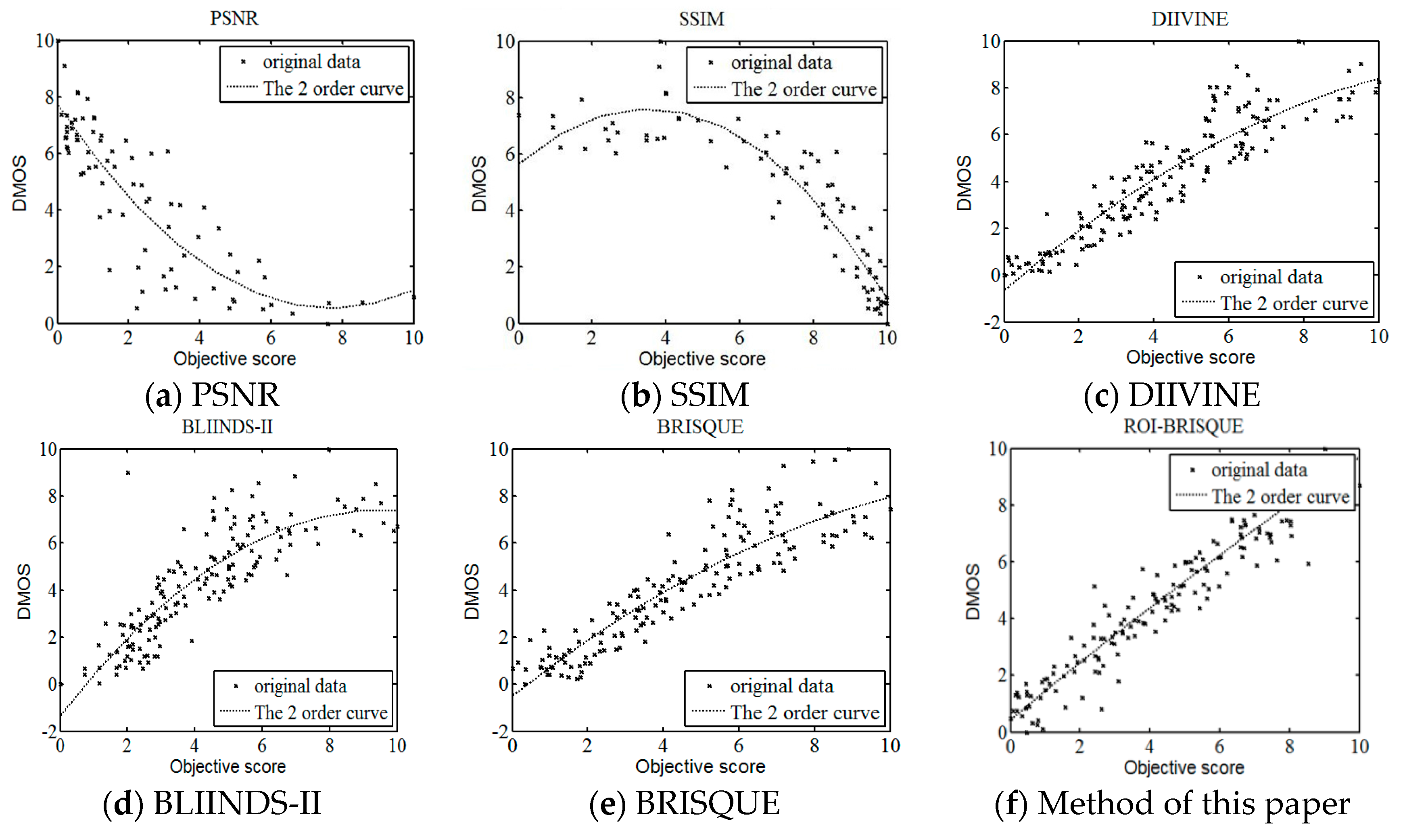
Usually we hope the scatter plot should define a cluster, that means the subjective score and objective evaluating score are tightly correlative since the ideal IQA algorithm should accurately reflect the subjective score, such as the DMOS [49]. The scatter plots of different IQA models are shown in Figure 13, where each point represents one test image, with its vertical and horizontal axes representing its predict score and the given objective quality score, respectively. We can see the scatter plots of full reference methods PSNR and SSIM are scattered, while the scatter plots of no reference methods DIIVINE, BLIINDS-II and BRISQUE are evenly distributed along the curve in the low distortion. The prediction is relatively accurate. When the degree of distortion of the image is too large, there is a deviation between the prediction results and the true value, scatter points more dispersed. In this paper, the method can accurately predict the image with different degree of distortion. We can see the distributions cluster along the curve.
In order to verify the accuracy of the method proposed in this paper further, we test five categories image distortion of LIVE image respectively. In addition, 100 images of various types are randomly selected to experiment. We list the median performance parameters for each distortion category and the overall parameters as well. The results are shown in Table 5.
As a whole it is obvious that ROI-BRISQUE performs well in terms of correlation with human perception, and is competitive with the BRISQUE across distortion types. From Table 5, it can be seen that the ROI-BRISQUE algorithm outperforms the BRISQUE indices in the five different types of distortion. This is a remarkable result, as it shows that algorithms that operate without any reference information can offer performance competitive with the predominant IQA algorithm over the last decades. Figure 14 is scatter plots of five categories. It can be shown that the proposed method has higher accuracy and stability than conventional image quality evaluation methods.
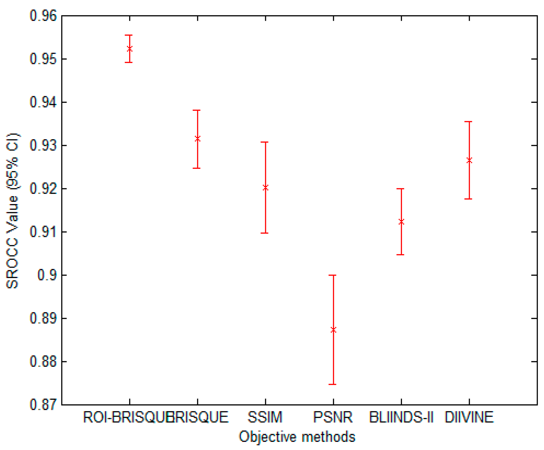
We also listed the median correlation values of ROI-BRISQUE as well as other PSNR, SSIM DIIVINE, BLIINDS-II and BRISQUE algorithms. Although the experiment results show some differences according to the median correlation, in this part we evaluate if these differences in correlation is statistically significant. To visualize the statistical significance of the comparison, we show error bars of the distribution of the SROCC values for each of the 1000 experimental trials. The error bars indicate the 95% confidence interval for each algorithm [50]. Plots are shown in Figure 15. Obviously, the lower the confidence interval with a higher median SROCC, the better the performance is. The plots show that the ROI-BRISQUE is not statistically significantly different in performance. In addition, in order to evaluate the statistical significance of performance of each algorithm, we use one-sided t-test between those correlation values [50]. We tabulate the results of such statistical analysis in Table 6. The null hypothesis is that the mean correlation for the row is equal to the mean correlation for the column at the 95% confidence level [51]. The other hypothesis is that the mean correlation of the row is greater or lesser than the mean correlation of the column. In the Table 6, the value of “1” indicates that the row method is statically superior to the column method, “−1” indicates that the row method is inferior to the column method, and “0” indicates that the row and the column methods are equivalent.
7.2.3. Database Independence
Since ROI-BRISQUE algorithm is evaluated only on the LIVE IQA database2, we cannot make sure that the performance of ROI-BRISQUE maintains its superiority in other IQA database. To show this, we apply the ROI-BRISQUE to the alternate TID2013 database [52]. The TID2013 database contains 25 reference images and 3000 distorted images (25 reference images × 24 types of distortions × 5 levels of distortions). Further, although it has 24 distortion categories, we test the ROI-BRISQUE only on these categories which has been trained for JPEG, JP2k (JPEG2000 compression), BLUR (Gaussian Blur), and WN (Additive white noise). TID2013 database does not contain FF (Fast Fading) distortion. The results of testing on TID2013 database are shown in Table 7. Compared with PSNR, SSIM, BLIINDS-II, DIIVINE and BRISQUE, the correlation with subjective perception of ROI-BRISQUE remained consistently competitive.
In addition, to study whether the algorithm is database dependent, we also test ROI-BRISQUE on a portion of the CSIQ image database [53]. The database consists of 30 original images, each distorted using one of six types of distortions, each at four to five different levels of distortion. The database contains 5000 subjective ratings from 35 different observers, and the ratings are reported in the form of DMOS (the value is in the range [0, 1], where 1 denotes the lowest quality). The distortions used in CSIQ are: JPEG compression, JPEG2000 compression, global contrast decrements, additive pink Gaussian noise, and Gaussian blurring. In total, there are 866 distorted images. We test ROI-BRISQUE on the CSIQ database over 4 distortion categories in common with the LIVE database: JPEG, JPEG2000, Gaussian noise, and Gaussian blurring. The experimental results are reported in Table 8. It is obvious that the performance of ROI-BRISQUE does not depend on the database. The correlations are still consistently high.
8. Conclusions
With the development of information technology, digital images have been widely used in every corner of our life and work, the research of image quality assessment algorithm also has very important practical significance. In this letter, we describe a framework for constructing an objective no-reference image quality assessment measure. The framework is unique, since it absorbs the features of human visual system. On the basis of human visual attention mechanism and BRISQUE method, this paper proposes a new NR IQA method based on visual perception, which we named as ROI-BRISQUE. First, we detailed the algorithm and the extraction model of ROI, and demonstrated the ROI consistent quite well with human perception. Then, we used BRISQUE method to extract image features and evaluated the ROI-BRISQUE index in terms of correlation with subjective quality score, and demonstrated that algorithm is statistically better than some state of the art IQA indices. At last, we demonstrated that ROI-BRISQUE performs consistently across different databases with similar distortions.
Further, the experimental results show that the new ROI-BRISQUE algorithm can be easily trained for a LIVE IQA database. In addition, it may be easily extended beyond the distortions considered here making it suitable for general-purpose blind IQA problems. The method correlates highly with visual perception of quality, and outperforms the full-reference PSNR and SSIM measure and the recent no-reference BLIINDS-II, DIIVINE indexes, and excels the performance of the no-reference BRISQUE index.
In the future, we will make further efforts to improve ROI-BRISQUE, such as further exploring human visual system and extracting the region of interest accurately.
Author Contributions
Both authors contributed equally to this work. Yan Fu and Shengchun Wang conceived this novel algorithm. Shengchun Wang performed the experiments and analyzed the data. Yan Fu tested the novel algorithm. Shengchun Wang wrote the paper, and Yan Fu revised the paper. Both authors have read and approved the final manuscript.
Conflicts of Interest
The authors declare no conflict of interest.
References
- Liu, L.; Dong, H.; Huang, H.; Bovik, A.C. No-reference image quality assessment in curvelet domain. Signal Process. Image Commun. 2014, 29, 494–505. [Google Scholar] [CrossRef]
- Hu, A.; Zhang, R.; Yin, D.; Zhan, Y. Image quality assessment using a SVD-based structural projection. Signal Process. Image Commun. 2014, 29, 293–302. [Google Scholar] [CrossRef]
- Liu, L.; Liu, B.; Huang, H.; Bovik, A.C. No-reference image quality assessment based on spatial and spectral entropies. Signal Process. Image Commun. 2014, 29, 856–863. [Google Scholar] [CrossRef]
- Requirements for an Objective Perceptual Multimedia Quality Model. Available online: https://www.itu.int/rec/T-REC-J.148-200305-I/en (accessed on 13 December 2016).
- Wang, Z.; Bovik, A.C.; Sheikh, H.R.; Simoncelli, E.P. Image quality assessment: From error visibility to structural similarity. IEEE Trans. Image Process. 2004, 13, 600–612. [Google Scholar] [CrossRef] [PubMed]
- Wang, Z.; Simoncelli, E.P.; Bovik, A.C. Multiscale structural similarity for image quality assessment. Signals Syst. Comput. 2003, 2, 1398–1402. [Google Scholar]
- Chandler, D.M.; Hemami, S.S. VSNR: A wavelet-based visual signal-to-noise ratio for natural images. IEEE Trans. Image Process. 2007, 16, 2284–2298. [Google Scholar] [CrossRef] [PubMed]
- Saad, M.A.; Bovik, A.C.; Charrier, C. A DCT statistics-based blind image quality index. Signal Process. Lett. 2010, 17, 583–586. [Google Scholar] [CrossRef]
- Pedersen, M.; Hardeberg, J.Y. Using gaze information to improve image difference metrics. Proc. SPIE Int. Soc. Opt. Eng. 2008, 6806, 97–104. [Google Scholar]
- Liu, H.; Heynderickx, I. Visual Attention in Objective Image Quality Assessment: Based on Eye-Tracking Data. IEEE Trans. Circuits Syst. Video Technol. 2011, 21, 971–982. [Google Scholar]
- Wang, B.; Wang, Z.; Liao, Y.; Lin, X. HVS-based structural similarity for image quality assessment. In Proceedings of the International Conference on Signal Processing, Beijing, China, 26–29 October 2008.
- Babu, R.V.; Perkis, A. An HVS-based no-reference perceptual quality assessment of JPEG coded images using neural networks. IEEE Int. Conf. Image Process. 2005, 1, I-433-6. [Google Scholar]
- Zhang, Y.D.; Wu, L.N.; Wang, S.H.; Wei, G. Color image enhancement based on HVS and PCNN. Sci. Chin. Inf. Sci. 2010, 53, 1963–1976. [Google Scholar] [CrossRef]
- Zhang, S.; Zhang, C.; Zhang, T.; Lei, Z. Review on universal no-reference image quality assessment algorithm. Comput. Eng. Appl. 2015, 51, 13–23. [Google Scholar]
- Feng, X.J.; Allebach, J.P. Measurement of ringing artifacts in JPEG images. Proc. Spie 2006, 6076, 74–83. [Google Scholar]
- Meesters, L.; Martens, J.B. A single-ended blockiness measure for JPEG-coded images. Signal Proc. 2002, 82, 369–387. [Google Scholar] [CrossRef]
- Wang, Z.; Sheikh, H.R.; Bovik, A.C. No-reference perceptual quality assessment of JPEG compressed images. Proc. IEEE Int. Conf. Image Process. 2003, 1, I-477–I-480. [Google Scholar]
- Shan, S. No-reference visually significant blocking artifact metric for natural scene images. Signal Proc. 2009, 89, 1647–1652. [Google Scholar]
- Tong, H.; Li, M.; Zhang, H.J.; Zhang, C. No-reference quality assessment for JPEG2000 compressed images. Int. Conf. Image Process. 2004, 5, 3539–3542. [Google Scholar]
- Marziliano, P.; Dufaux, F.; Winkler, S.; Ebrahimi, T. Perceptual blur and ringing metrics: Application to JPEG2000. Signal Process. Image Commun. 2004, 19, 163–172. [Google Scholar] [CrossRef]
- Sazzad, Z.M.P.; Kawayoke, Y.; Horita, Y. No reference image quality assessment for JPEG2000 based on spatial features. Signal Process. Image Commun. 2008, 23, 257–268. [Google Scholar] [CrossRef]
- Sheikh, H.R.; Bovik, A.C.; Cormack, L. No-reference quality assessment using natural scene statistics: JPEG2000. IEEE Trans. Image Process. 2005, 14, 1918–1927. [Google Scholar] [CrossRef] [PubMed]
- Caviedes, J.; Oberti, F. A new sharpness metric based on local kurtosis, edge and energy information. Signal Process. Image Commun. 2004, 19, 147–161. [Google Scholar] [CrossRef]
- Ferzli, R.; Karam, L.J. A no-reference objective image sharpness metric based on the notion of Just Noticeable Blur (JNB). IEEE Trans. Image Process. 2009, 18, 717–728. [Google Scholar] [CrossRef] [PubMed]
- Sang, Q.B.; Su, Y.Y.; Li, C.F.; Wu, X.J. No-reference blur image quality assessment based on gradient similarity. J. Optoelectron. Laser 2013, 24, 573–577. [Google Scholar]
- Moorthy, A.K.; Bovik, A.C. A two-step framework for constructing blind image quality indices. Signal Process. Lett. 2010, 17, 513–516. [Google Scholar] [CrossRef]
- Moorthy, A.K.; Bovik, A.C. Blind image quality assessment: From natural scene statistics to perceptual quality. IEEE Trans. Image Process. 2011, 20, 3350–3364. [Google Scholar] [CrossRef] [PubMed]
- Saad, M.A.; Bovik, A.C.; Charrier, C. DCT statistics model based blind image quality assessment. In Proceedings of the 18th IEEE International Conference on Image Processing (ICIP), Brussels, Belgium, 11–14 September 2011.
- Mittal, A.; Moorthy, A.K.; Bovik, A.C. No-reference image quality assessment in the spatial domain. IEEE Trans. Image Process. 2012, 21, 4695–4708. [Google Scholar] [CrossRef] [PubMed]
- Ruderman, D.L. The statistics of natural images. Netw. Comput. Neural Syst. 1994, 5, 517–548. [Google Scholar] [CrossRef]
- Mittal, A.; Soundararajan, R.; Bovik, A.C. Making a “completely blind” image quality analyzer. Signal Process. Lett. 2013, 20, 209–212. [Google Scholar] [CrossRef]
- Zhang, L.; Shen, Y.; Li, H. VSI: A visual saliency-induced index for perceptual image quality assessment. IEEE Trans. Image Process. Publ. IEEE Signal Process. Soc. 2014, 23, 4270–4281. [Google Scholar] [CrossRef] [PubMed]
- Itti, L.; Koch, C.; Niebur, E. A model of saliency-based visual attention for rapid scene analysis. IEEE Trans. Pattern Anal. Mach. Intell. 1998, 20, 1254–1259. [Google Scholar] [CrossRef]
- Itti, L.; Koch, C. Computational modeling of visual attention. Nat. Rev. Neurosci. 2001, 2, 194–230. [Google Scholar] [CrossRef] [PubMed]
- Itti, L.; Koch, C. Feature combination strategies for saliency based visual attention systems. J. Electr. Imaging 2001, 10, 161–169. [Google Scholar] [CrossRef]
- Navalpakkam, V.; Itti, L. An integrated model of top-down and bottom-up attention for optimizing detection speed. In Proceedings of the IEEE Computer Society Conference on Computer Vision and Pattern Recognition, New York, NY, USA, 17–22 June 2006.
- Schölkopf, B.; Platt, J.; Hofmann, T. Graph-Based Visual Saliency. Adv. Neural Inf. Process. Syst. 2006, 19, 545–552. [Google Scholar]
- Sheikh, H.R.; Wang, Z.; Cormack, L.; Bovik, A.C. Live Image Quality Assessment Database Release 2. Available online: http://live.ece.utexas.edu/research/quality/subjective.htm (accessed on 13 December 2016).
- Zhang, Y.; Dong, Z.; Wang, S.; Ji, G.; Yang, J. Preclinical Diagnosis of Magnetic Resonance (MR) Brain Images via Discrete Wavelet Packet Transform with Tsallis Entropy and Generalized Eigenvalue Proximate Support Vector Machine (GEPSVM). Entropy 2015, 17, 1795–1813. [Google Scholar] [CrossRef]
- Wang, S.; Lu, S.; Dong, Z.; Yang, J.; Yang, M.; Zhang, Y. Dual-Tree Complex Wavelet Transform and Twin Support Vector Machine for Pathological Brain Detection. Appl. Sci. 2016, 6, 169. [Google Scholar] [CrossRef]
- Barina, D. Gabor Wavelets in Image Processing. 2016; arXiv:1602.03308. [Google Scholar]
- Sharifi, K.; Leon-Garcia, A. Estimation of shape parameter for generalized Gaussian distributions in sub-band decompositions of video. IEEE Trans. Circuits Syst. Video Technol. 1995, 5, 52–56. [Google Scholar] [CrossRef]
- Wainwright, M.J.; Simoncelli, E.P. Scale mixtures of Gaussians and the statistics of natural images. Neural Inf. Process. Syst. 2000, 12, 855–861. [Google Scholar]
- Lasmar, N.E.; Stitou, Y.; Berthoumieu, Y. Multiscale skewed heavy tailed model for texture analysis. In Proceedings of the 16th IEEE International Conference on Image Processing (ICIP), Cairo, Egypt, 7–10 November 2009.
- Alers, H.; Liu, H.; Redi, J.; Heynderickx, I. TUD Image Quality Database: Eye-Tracking Release 2. Available online: http://mmi.tudelft.nl/iqlab/eye_tracking_2.html (accessed on 13 December 2016).
- Alers, H.; Liu, H.; Redi, J.; Heynderickx, I. Studying the risks of optimizing the image quality in saliency regions at the expense of background content. In Proceedings of the IS & T/SPIE Electronic Imaging 2010, Image Quality and System Performance VII, San Jose, CA, USA, 17–21 January 2010.
- Sheikh, H.R.; Sabir, M.F.; Bovik, A.C. A Statistical Evaluation of Recent Full Reference Image Quality Assessment Algorithms. IEEE Trans. Image Process. 2006, 15, 3440–3451. [Google Scholar] [CrossRef] [PubMed]
- Chang, C.C.; Lin, C.J. LIBSVM: A library for support vector machines. ACM Trans. Intell. Syst. Technol. 2011, 2, 389–396. [Google Scholar] [CrossRef]
- Tong, Y.; Konik, H.; Cheikh, F.A.; Tremeau, A. Full Reference Image Quality Assessment Based on Saliency Map Analysis. J. Imaging Sci. Technol. 2010, 54, 3. [Google Scholar] [CrossRef]
- Sheskin, D.J. Handbook of Parametric and Nonparametric Statistical Procedures, 3rd ed.; Statistical Procedures: Boca, FL, USA, 2012. [Google Scholar]
- Steiger, J.H. Beyond the F Test: Effect Size Confidence Intervals and Tests of Close Fit in the Analysis of Variance and Contrast Analysis. Psychol. Methods 2004, 9, 164–182. [Google Scholar] [CrossRef] [PubMed]
- Ponomarenko, N.; Ieremeiev, O.; Lukin, V.; Egiazarian, K.; Jin, L.; Astola, J.; Vozel, B.; Chehdi, K.; Carli, M.; Battisti, F.; et al. Color image database TID2013: Peculiarities and preliminary results. In Proceedings of the European Workshop on Visual Information Processing, Paris, France, 10–12 June 2013.
- Larson, E.C.; Chandler, D.M. Most apparent distortion: Full-reference image quality assessment and the role of strategy. J. Electr. Imaging 2010, 19, 143–153. [Google Scholar]
Figure 1.
General architecture of the model.

Figure 2.
Improved architecture of the mode.
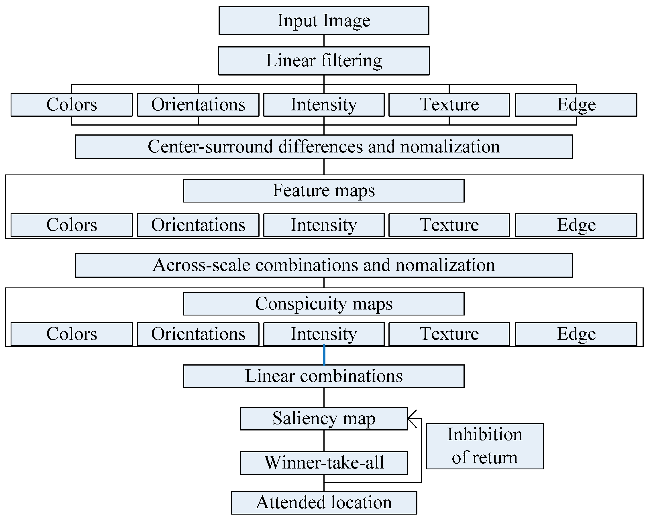
Figure 3.
Frequency component of Gabor filter.

Figure 4.
Gabor wavelet based on different directions. (a) θ = 0, (b) θ = π/4, (c) θ = π/2, (d) θ = 3 × π/4.
Figure 4.
Gabor wavelet based on different directions. (a) θ = 0, (b) θ = π/4, (c) θ = π/2, (d) θ = 3 × π/4.
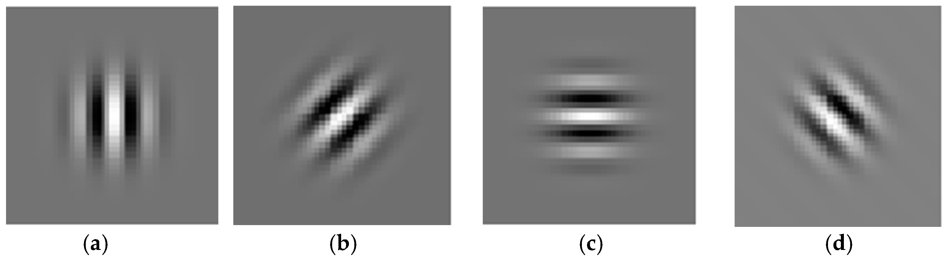
Figure 5.
Damaged figure of non-interest region.

Figure 6.
Damaged figure of interest region.

Figure 7.
Model of Region of Interest—Blind/Reference Image Spatial Quality Evaluator.

Figure 8.
Comparison of different visual saliency models. (a) Original image; (b–d) salient overlap maps of GBVS model, Itti model and improved Itti model respectively; (e–g) salient maps of GBVS model, Itti model and improved Itti model respectively.
Figure 8.
Comparison of different visual saliency models. (a) Original image; (b–d) salient overlap maps of GBVS model, Itti model and improved Itti model respectively; (e–g) salient maps of GBVS model, Itti model and improved Itti model respectively.


Figure 9.
Comparison of different visual saliency models. (a) Original image; (b–d) salient overlap maps of GBVS model, Itti model and improved Itti model respectively; (e–g) salient maps of GBVS model, Itti model and improved Itti model respectively.
Figure 9.
Comparison of different visual saliency models. (a) Original image; (b–d) salient overlap maps of GBVS model, Itti model and improved Itti model respectively; (e–g) salient maps of GBVS model, Itti model and improved Itti model respectively.

Figure 10.
Comparison of different visual saliency models. (a) Original image; (b–d) salient overlap maps of GBVS model, Itti model and improved Itti model respectively; (e–g) salient maps of GBVS model, Itti model and improved Itti model respectively.
Figure 10.
Comparison of different visual saliency models. (a) Original image; (b–d) salient overlap maps of GBVS model, Itti model and improved Itti model respectively; (e–g) salient maps of GBVS model, Itti model and improved Itti model respectively.

Figure 11.
Comparison of different visual saliency models. (a) Original image; (b–d) salient overlap maps of GBVS model, Itti model and improved Itti model respectively; (f–h) salient maps of GBVS model, Itti model and improved Itti model respectively; (e) Salient map of free looking task; (i) salient map of scoring task.
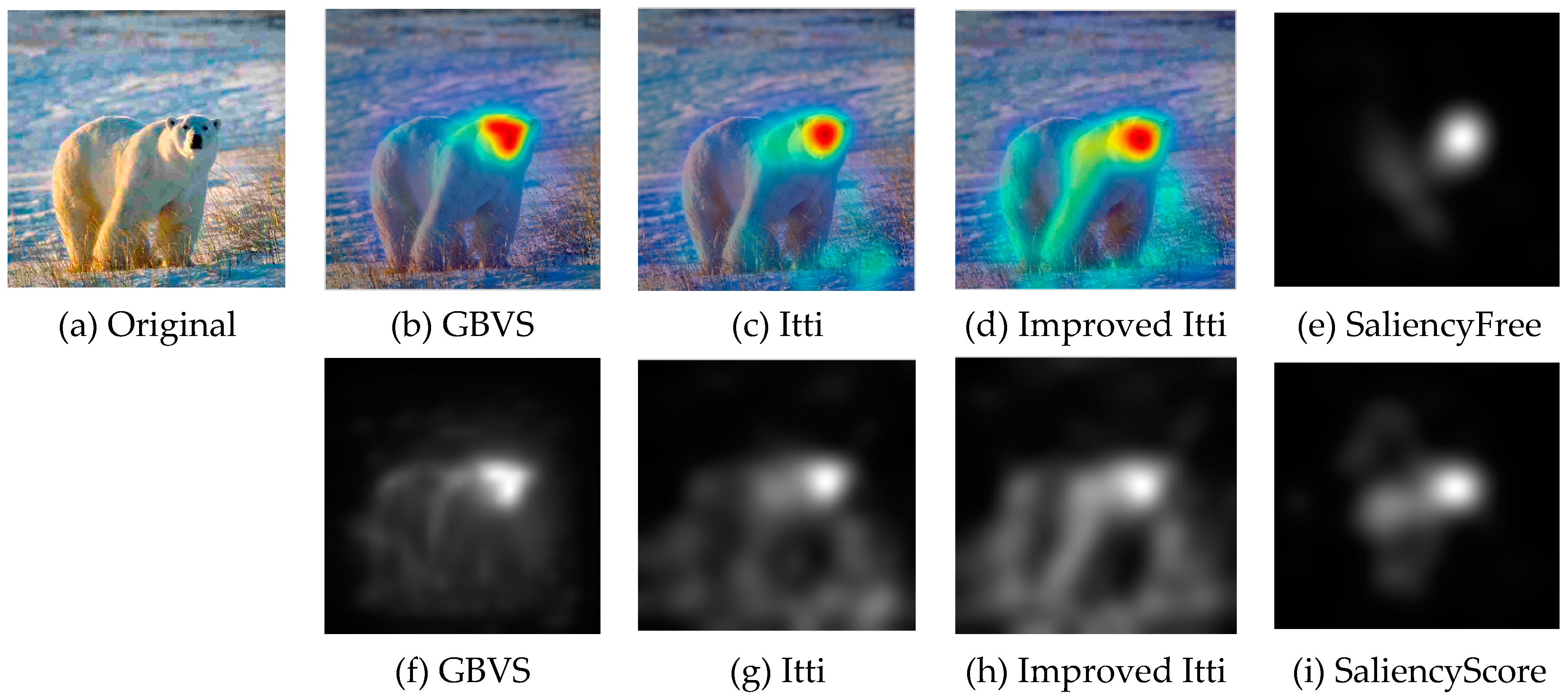
Figure 12.
Comparison of different visual saliency models. (a) Original image; (b–d) salient overlap maps of GBVS model, Itti model and improved Itti model respectively; (f–h) salient maps of GBVS model, Itti model and improved Itti model respectively; (e) Salient map of free looking task; (i) salient map of scoring task

Figure 13.
Scatter plots of DMOS versus different model predictions. Each sample point represents one test image in the entire LIVE database. (a) PSNR model; (b) SSIM model; (c) DIIVINE model; (d) BLIINDS-II model; (e) BRISQUE model; (f) Model of this paper (ROI-BRISQUE).
Figure 13.
Scatter plots of DMOS versus different model predictions. Each sample point represents one test image in the entire LIVE database. (a) PSNR model; (b) SSIM model; (c) DIIVINE model; (d) BLIINDS-II model; (e) BRISQUE model; (f) Model of this paper (ROI-BRISQUE).

Figure 14.
Scatter plots of JPEG, JP2k, WN, BLUR and FF. Scatter plots of predicted score versus subjective DMOS on LIVE IQA database. (a) JPEG database subset; (b) JPEG2000 database subset; (c) Gaussian white noise database subset; (d) Gaussian blur database subset; (e) fast-fading database subset.
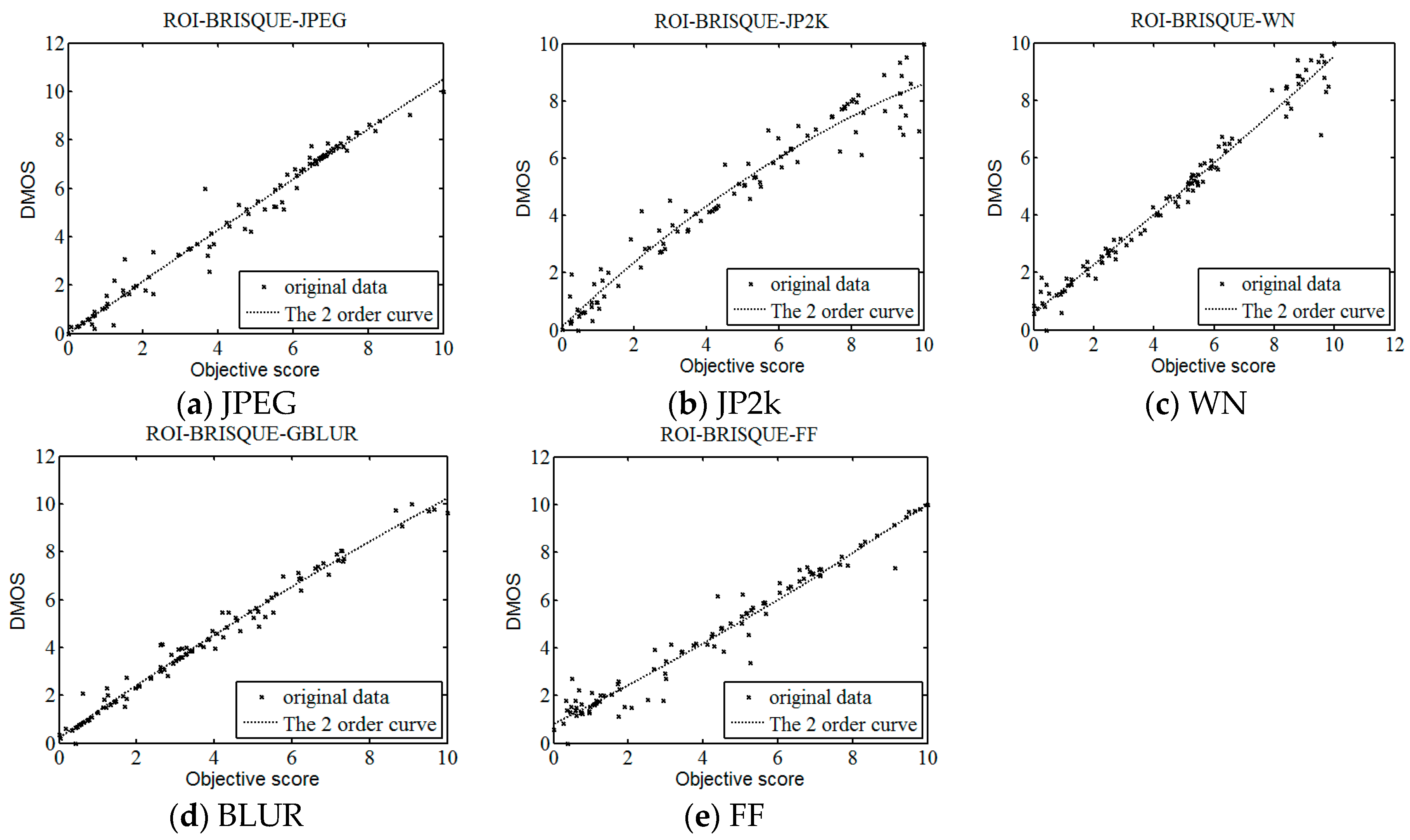
Figure 15.
Mean SROCC value of the algorithms evaluated in Table 4, across 1000 train-test on the LIVE IQA database2. The error bars indicate the 95% confidence interval.
Figure 15.
Mean SROCC value of the algorithms evaluated in Table 4, across 1000 train-test on the LIVE IQA database2. The error bars indicate the 95% confidence interval.

Table 1.
Performance of ROI-BRISQUE which ROI extracted by the improved Itti model. The numbers in bold are the best values.
| λ | KROCC | RMSE | SROCC | PLCC |
|---|---|---|---|---|
| 0.0 | 0.7674 | 7.9544 | 0.8805 | 0.8818 |
| 0.1 | 0.7692 | 7.7801 | 0.8936 | 0.8958 |
| 0.2 | 0.7725 | 6.9801 | 0.9169 | 0.9220 |
| 0.3 | 0.7802 | 6.2725 | 0.9234 | 0.9267 |
| 0.4 | 0.7816 | 5.9544 | 0.9303 | 0.9352 |
| 0.5 | 0.7899 | 5.5036 | 0.9439 | 0.9459 |
| 0.6 | 0.7907 | 5.0113 | 0.9443 | 0.9450 |
| 0.7 | 0.8021 | 4.7825 | 0.9495 | 0.9494 |
| 0.8 | 0.7981 | 4.9130 | 0.9493 | 0.9482 |
| 0.9 | 0.7910 | 5.1800 | 0.9454 | 0.9444 |
| 1.0 | 0.7841 | 5.5767 | 0.9413 | 0.9396 |
Table 2.
Performance of ROI-BRISQUE which ROI extracted by Itti model. The numbers in bold are the best values in the corresponding column.
| λ | KROCC | RMSE | SROCC | PLCC |
|---|---|---|---|---|
| 0.0 | 0.7452 | 7.0713 | 0.9059 | 0.8998 |
| 0.1 | 0.7585 | 6.6507 | 0.9175 | 0.9119 |
| 0.2 | 0.7714 | 6.3002 | 0.9269 | 0.9214 |
| 0.3 | 0.7829 | 5.9391 | 0.9352 | 0.9304 |
| 0.4 | 0.7926 | 5.7110 | 0.9407 | 0.9354 |
| 0.5 | 0.7916 | 5.7155 | 0.9412 | 0.9353 |
| 0.6 | 0.7849 | 5.7062 | 0.9378 | 0.9356 |
| 0.7 | 0.7848 | 5.6635 | 0.9376 | 0.9365 |
| 0.8 | 0.7736 | 5.9682 | 0.9299 | 0.9294 |
| 0.9 | 0.7572 | 6.3446 | 0.9196 | 0.9200 |
| 1.0 | 0.7509 | 6.4869 | 0.9145 | 0.9162 |
Table 3.
Performance of ROI-BRISQUE which ROI extracted by GBVS model. The numbers in bold are the best values.
| λ | KROCC | RMSE | SROCC | PLCC |
|---|---|---|---|---|
| 0.0 | 0.7490 | 6.7257 | 0.9175 | 0.9102 |
| 0.1 | 0.7592 | 6.3346 | 0.9258 | 0.9207 |
| 0.2 | 0.7709 | 6.0183 | 0.9321 | 0.9288 |
| 0.3 | 0.7938 | 5.5164 | 0.9432 | 0.9401 |
| 0.4 | 0.7991 | 5.3783 | 0.9453 | 0.9433 |
| 0.5 | 0.7938 | 5.5856 | 0.9439 | 0.9392 |
| 0.6 | 0.7918 | 5.5501 | 0.9429 | 0.9399 |
| 0.7 | 0.7890 | 5.5012 | 0.9400 | 0.9409 |
| 0.8 | 0.7880 | 5.5172 | 0.9404 | 0.9405 |
| 0.9 | 0.7804 | 5.6695 | 0.9371 | 0.9372 |
| 1.0 | 0.7745 | 5.8075 | 0.9341 | 0.9345 |
Table 4.
Performance comparison of some IQA methods and the method of this paper. Italicized algorithms are NR IQA algorithms, others are FR IQA algorithms.
| KROCC | RMSE | SROCC | PLCC | |
|---|---|---|---|---|
| PSNR | 0.6674 | 11.2795 | 0.8873 | 0.8866 |
| SSIM | 0.7410 | 10.5723 | 0.9201 | 0.9110 |
| BLIINDS-II | 0.7619 | 9.8894 | 0.9123 | 0.9145 |
| DIIVINE | 0.7643 | 8.1542 | 0.9265 | 0.9283 |
| BRISQUE | 0.7768 | 6.5468 | 0.9314 | 0.9377 |
| ROI-BRISQUE | 0.8021 | 4.7613 | 0.9522 | 0.9465 |
| JPEG | JP2K | BLUR | WN | FF | ALL | ||
|---|---|---|---|---|---|---|---|
| RMSE | ROI-BRISQUE | 2.5975 | 3.9836 | 2.2188 | 2.6453 | 3.9494 | 4.7613 |
| BRISQUE | 4.0339 | 5.4350 | 4.0374 | 3.3340 | 5.6078 | 6.5468 | |
| KROCC | ROI-BRISQUE | 0.8071 | 0.7927 | 0.8384 | 0.8933 | 0.7398 | 0.8021 |
| BRISQUE | 0.7691 | 0.7619 | 0.8286 | 0.8792 | 0.7237 | 0.7768 | |
| PLCC | ROI-BRISQUE | 0.9867 | 0.9693 | 0.9801 | 0.9927 | 0.9719 | 0.9465 |
| BRISQUE | 0.9551 | 0.9090 | 0.9498 | 0.9903 | 0.9148 | 0.9377 | |
| SROCC | ROI-BRISQUE | 0.9858 | 0.9690 | 0.9865 | 0.9908 | 0.9561 | 0.9522 |
| BRISQUE | 0.9647 | 0.9139 | 0.9479 | 0.9843 | 0.9053 | 0.9314 | |
Table 6.
Results of one-sided t-test performed between SROCC values of various IQA algorithms. The value of “1” indicates that the row algorithm is statically superior to the column algorithm; “−1” indicates that the row is inferior to the column; “0” indicates that the row and the column methods are equivalent. Italics indicate No-reference algorithms.
| PSNR | SSIM | BLIINDS-II | DIIVINE | BRISQUE | ROI-BRISQUE | |
|---|---|---|---|---|---|---|
| PSNR | 0 | −1 | −1 | −1 | −1 | −1 |
| SSIM | 1 | 0 | 1 | −1 | −1 | −1 |
| BLIINDS-II | 1 | −1 | 0 | −1 | −1 | −1 |
| DIIVINE | 1 | 1 | 1 | 0 | −1 | −1 |
| BRISQUE | 1 | 1 | 1 | 1 | 0 | −1 |
| ROI-BRISQUE | 1 | 1 | 1 | 1 | 1 | 0 |
Table 7.
SROCC results obtained by training on the LIVE IQA database and testing on the TID2013 database. Italicized algorithms are NR IQA algorithms, others are FR IQA algorithms.
| JP2K | JPEG | WN | BLUR | All | |
|---|---|---|---|---|---|
| PSNR | 0.8250 | 0.8760 | 0.9180 | 0.9342 | 0.8700 |
| SSIM | 0.9630 | 0.9354 | 0.8168 | 0.9600 | 0.9016 |
| BLIINDS-II | 0.9157 | 0.8901 | 0.6600 | 0.8500 | 0.8442 |
| DIIVINE | 0.9240 | 0.8660 | 0.8510 | 0.8620 | 0.8890 |
| BRISQUE | 0.8320 | 0.9240 | 0.8290 | 0.8810 | 0.8960 |
| ROI-BRISQUE | 0.8534 | 0.9276 | 0.8488 | 0.8965 | 0.8993 |
Table 8.
SROCC results obtained by training on the LIVE IQA database and testing on the CSIQ database. Italicized algorithms are NR IQA algorithms, others are FR IQA algorithms.
| JP2K | JPEG | WN | BLUR | All | |
|---|---|---|---|---|---|
| PSNR | 0.8905 | 0.8993 | 0.9173 | 0.8620 | 0.8810 |
| SSIM | 0.9606 | 0.9546 | 0.8922 | 0.9609 | 0.9420 |
| BLIINDS-II | 0.9057 | 0.8809 | 0.6956 | 0.8653 | 0.8452 |
| DIIVINE | 0.8084 | 0.8673 | 0.8594 | 0.8312 | 0.8472 |
| BRISQUE | 0.8662 | 0.8394 | 0.8253 | 0.8625 | 0.8509 |
| ROI-BRISQUE | 0.8869 | 0.8404 | 0.8277 | 0.8689 | 0.8553 |
© 2016 by the authors; licensee MDPI, Basel, Switzerland. This article is an open access article distributed under the terms and conditions of the Creative Commons Attribution (CC-BY) license (http://creativecommons.org/licenses/by/4.0/).
Share and Cite
MDPI and ACS Style
Fu, Y.; Wang, S. A No Reference Image Quality Assessment Metric Based on Visual Perception. Algorithms 2016, 9, 87. https://doi.org/10.3390/a9040087
AMA Style
Fu Y, Wang S. A No Reference Image Quality Assessment Metric Based on Visual Perception. Algorithms. 2016; 9(4):87. https://doi.org/10.3390/a9040087
Chicago/Turabian StyleFu, Yan, and Shengchun Wang. 2016. "A No Reference Image Quality Assessment Metric Based on Visual Perception" Algorithms 9, no. 4: 87. https://doi.org/10.3390/a9040087
Note that from the first issue of 2016, this journal uses article numbers instead of page numbers. See further details here.