Analysis of Climate Change Impacts on Tree Species of the Eastern US: Results of DISTRIB-II Modeling


1
USDA Forest Service, Northern Research Station, Northern Institute of Applied Climate Science, Delaware, OH 43015, USA
2
School of Environment and Natural Resources, The Ohio State University, Columbus, OH 43210, USA
*
Author to whom correspondence should be addressed.
Forests 2019, 10(4), 302; https://doi.org/10.3390/f10040302
Submission received: 22 February 2019
/
Revised: 19 March 2019
/
Accepted: 27 March 2019
/
Published: 2 April 2019
(This article belongs to the Special Issue New Technical Advances: Explore Forest Landscape Ecology and Biodiversity Using Geographic Information Science)
Abstract
:Forests across the globe are faced with a rapidly changing climate and an enhanced understanding of how these changing conditions may impact these vital resources is needed. Our approach is to use DISTRIB-II, an updated version of the Random Forest DISTRIB model, to model 125 tree species individually from the eastern United States to quantify potential current and future habitat responses under two Representative Concentration Pathways (RCP 8.5 -high emissions which is our current trajectory and RCP 4.5 -lower emissions by implementing energy conservation) and three climate models. Climate change could have large impacts on suitable habitat for tree species in the eastern United States, especially under a high emissions trajectory. On average, of the 125 species, approximately 88 species would gain and 26 species would lose at least 10% of their suitable habitat. The projected change in the center of gravity for each species distribution (i.e., mean center) between current and future habitat moves generally northeast, with 81 species habitat centers potentially moving over 100 km under RCP 8.5. Collectively, our results suggest that many species will experience less pressure in tracking their suitable habitats under a path of lower greenhouse gas emissions.
1. Introduction
The climate is changing, globally becoming warmer almost every year in recent decades. Risks associated with this warming are high, sometimes manifesting into multiple, broad threats to humanity [1] and the economy [2]. The recent Intergovernmental Panel on Climate Change (IPCC) report on the impacts of global warming of 1.5 °C above pre-industrial levels, and in comparison to impacts of 2.0 °C, describes many ‘Reasons for Concern’ related to efforts to strengthen the global response to the threat of climate change, sustainable development, and efforts to eradicate poverty [3]. Even so, with current pledges in the Paris Agreement on Climate Change, ~2.6–3.2 °C of warming is projected by 2100, though the Agreement aims to limit global warming “well below 2 °C” and to “pursue efforts” to limit temperatures above pre-industrial levels to 1.5 °C [4]. The biodiversity implications of these various levels of warming are huge, as outlined in Warren, et al. [5], where climatically determined geographic range losses exceeding 50% were projected for 44%, 16%, and 8% of plants by 2100, corresponding to warming of 3.2, 2.0, and 1.5 °C, respectively. Even though climatically determined range losses do not equate with actual distributions of plants because trees live a long time while harboring great genetic diversity, the potential effects of climate change on the biota of the planet are staggering. Meanwhile, the co-benefits of limiting the amount of warming towards the 1.5 °C path are immense.
As a consequence of the range of these potential changes, models are needed to provide a suite of possible outcomes, by species, to assist decision makers to minimize biological impacts and to adapt to the coming changes. Adaptation planning has been accelerating, whether by motivation or mandate. For example, the Northern Institute of Applied Climate Science (NIACS), associated with the USDA Forest Service, has facilitated nearly 300 adaptation demonstrations or projects on forest lands over the last 10 years in the north central and northeastern United States via their Adaptation Workbook [6], www.forestadaptation.org. Model outputs are critical for understanding vulnerability and evaluating possible adaptation avenues, particularly when considering transitional or facilitated outcomes [7,8,9].
To arrive at reliable and informative models of how tree species may respond to a rapidly changing climate, a diverse and dynamic field has emerged, where continued refinement affords new insights. Statistical models and mechanistic models form a dichotomy of how one approaches predicting future change and each has their strengths and weaknesses [10,11]. Demography approaches add another useful dimension to modeling potential futures [12,13], as do paleoecologic studies [14,15]. Hybrid approaches, which use a combination of modeling methods, may also provide key insights not otherwise uncovered [16,17,18,19]. Nonetheless, primary themes from all modeling studies indicate the value of forests in the overall climate equation and the high potential for eventual forest composition and productivity changes in the future [20,21].
With passing time, the evidence is mounting that changes are indeed occurring in forest composition and productivity. Evidence of migration of tree species along elevational gradients (up or down) has been mounting for some time, along with the ecological explanations for such movements [22,23,24,25,26,27,28,29,30]. However, latitudinal or longitudinal changes in species range are more difficult to document because of wide distributions, limited sample size, and confounding disturbance factors, such as insect pests and succession following harvest, forest clearing, fire exclusion, human introductions, or other disturbance [21,31,32,33,34]. Nonetheless, recent studies conducted with repeated inventory and demography data do provide insights into changes (or not) in range limits. Boisvert-Marsh and others [35,36] found poleward shifts in Quebec, Canada for Acer saccharum Marshal, Acer rubrum L., Fagus grandifolia Ehrh., and Betula alleghaniensis Britt. between 1970–1977 and 2003–2014, mostly attributed to warming of early- or late-season climatic variables. However, they also detected southward shifts of Abies balsamea (L.) Mill., Picea glauca (Moench) Voss, and Picea mariana (Mill.) B.S.P., attributed to natural and human disturbances. Sittaro et al. [37], also in working in Quebec, found that the spatial velocity of temperature at range limits exceeded the pace of tree species migration by a factor of two for 14 of 16 species. Woodall and D’Amato [38], in a decadal evaluation of 20 eastern US tree species not extending north of the Canada border, found stability for 85% of the species, regardless of the level of canopy disturbance.
Our modeling approach has been to statistically model potential changes in suitable habitat for a large number to species using Forest Inventory and Analysis (FIA) data and environmental co-variates. This approach has evolved along with concomitant large advances in hardware, data, analytical software, and techniques. Our first effort for 80 common trees used county-level data and the statistical technique Regression Tree Analysis [39,40]. We then moved to a 20 × 20 km grid, 134 tree species, and the Random Forest technique [41,42,43], our original DISTRIB model which modeled suitable habitat for 134 tree species from the Eastern United States. These models were the basis for several NIACS reports on the vulnerability of forests to climate change in the Mid-Atlantic region [44], the Central Appalachians [45], the Central Hardwoods [46], the Northwoods of Minnesota [47], Michigan [48], and Wisconsin [49], New York and New England [50], and the Chicago Wilderness region [51]. Most recently, we have developed a new set of models based on newer FIA data (www.fia.fs.fed.us), higher resolution soils data [52], and a hybrid lattice composed of 10 × 10 km and 20 × 20 km grids, derived from FIA plot density and described in a subsequent paper. The objective of this paper is to summarize the outputs from the DISTRIB-II model, for 125 species of trees in the eastern United States.
2. Materials and Methods
In our effort reported here, we present summaries from our recent revision of the original DISTRIB model, now called DISTRIB-II. The extent of our analysis encompasses the United States east of the 100th meridian. In DISTRIB-II, we developed a hybrid lattice of a mix of 20 × 20 and 10 × 10 km cells. The mixture of cell sizes allowed us to optimize modeling by increasing resolution for those cells which had support from sufficient FIA plots. Locations, such as large parts of the Corn Belt in the Midwest, had few FIA plots, so we retained the coarser, 20-km structure, while those locations with higher densities of FIA plots were evaluated and modeled via a 10-km structure. DISTRIB-II also used completely updated data sets of 45 environmental variables and FIA plot data; it also used newer techniques to assign model output values.
2.1. Data
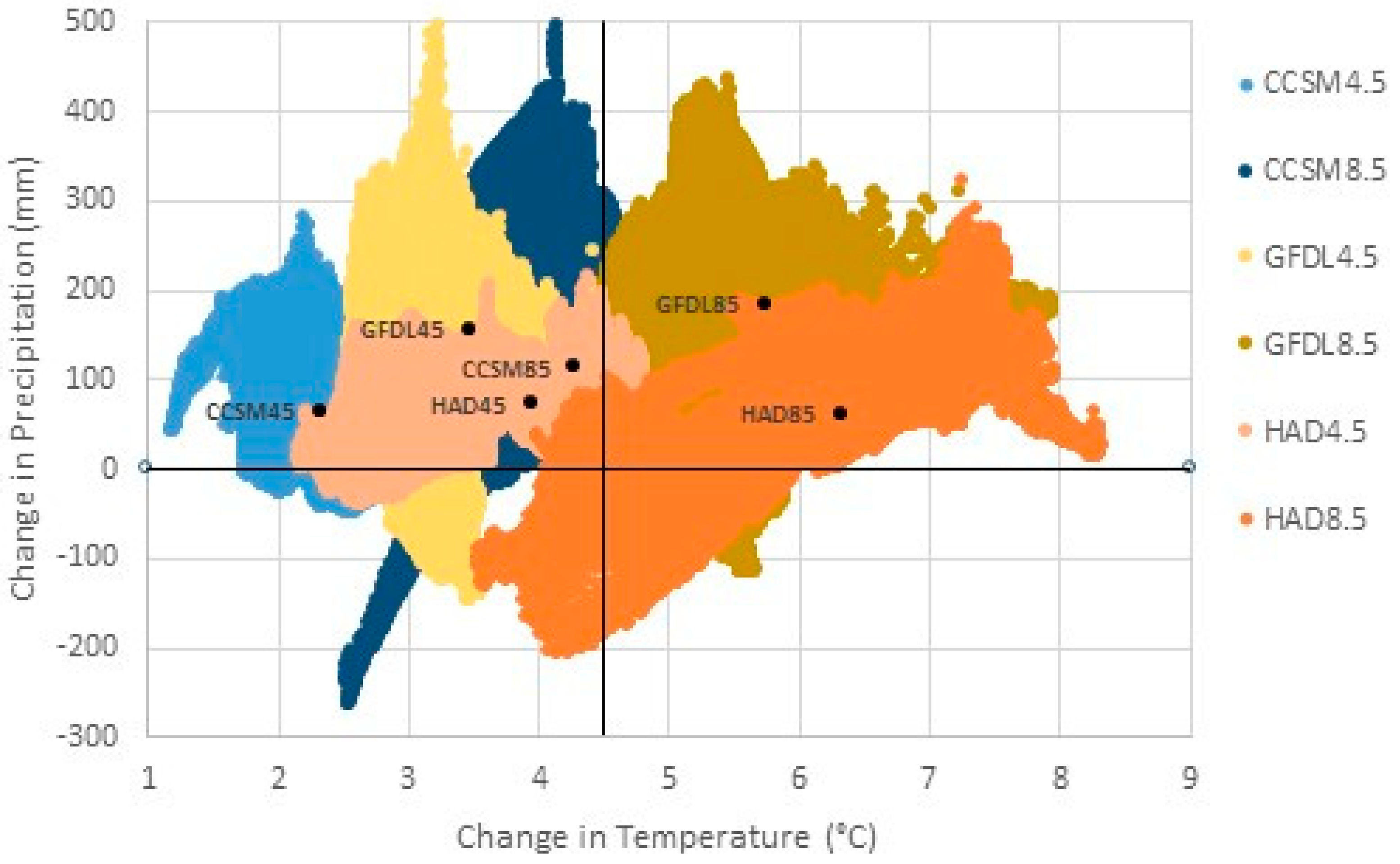
Climate data. We used a range of models and scenarios to capture projections of future temperature and precipitation. Data included current (1981–2010) annual and seasonal mean temperature (°C) and annual and seasonal precipitation totals (mm) based on Parameter-elevation Regressions on Independent Slopes Model, [53] (PRISM), and end of the century (2070–2099) projected mean values from three General Circulation Models (GCM) under the 4.5 and 8.5 Representative Concentration Pathways (RCP). Downscaled future projections were obtained from NASA Earth Exchange U.S. Downscaled Climate Projections (NEX-US-DCP30) project (https://cds.nccs.nasa.gov/nex/), with metadata found at (https://cds.nccs.nasa.gov/wp-content/uploads/2014/04/NEX-DCP30_Tech_Note_v0.pdf) [54]. These data are derived from GCM runs under the Coupled Model Inter-comparison Project Phase 5 (CMIP5) in support of the IPCC Fifth Assessment Report (IPCC AR5). The NEX US-DCP30 dataset was downscaled to 30 × 30 arcseconds via Bias-Correction Spatial Disaggregation (BCSD) [55]. Future values were derived by adjusting PRISM data with the change (the deltas) between GCM-simulated data for periods 1981–2010 and 2070–2099, similar to methods described by Monahan, et al. [56]. These delta adjustments provided closer alignment to current conditions now and minimized exposure to pixel-level artifacts between training and projection climate data. For climate summaries reported in Table 1, data were aggregated to 10-km across 41,681 cells across the eastern U.S. Three models were used, each with RCP 4.5 and 8.5 [57]: Community Climate System Model, or CCSM4 (hereafter CCSM45 and CCSM85) [58], Geophysical Fluid Dynamics Laboratory (Donner), or GFDL-CM3 (GFDL45 and GFDL85) [59], and Hadley Global Environment Model—Earth System [60] (or HadGEM2-ES (Had45 and Had85) [61]. These climate models and RCPs capture, for the entire eastern U.S. study area, a wide distribution space in projected change (Figure 1 and detailed in Table 1). Further, the mean change across these combinations (Figure 1), fall along a strong temperature gradient, from an estimated annual temperature increase of 2.5 °C with CCSM45 to 6.5 °C with Had85, and with an overall mean increase of 4.5 °C. The potential change in annual precipitation (though precipitation changes have higher uncertainty as compared to temperature changes) was higher for all scenarios by end of the century, but for many locations, a reduction in future precipitation is forecasted (i.e., points below the horizontal 0 change line), especially for Had85 and GFDL85 (Figure 1). Coupled with higher temperatures, especially these scenarios will likely inflict additional physiological stress on organisms for some future periods (see also [62]). This trend is especially true when examining growing season temperatures, which reach 28.4 °C, an increase of 6.8 °C, for both GFDL85 and Had85. To make matters worse for plant growth, the Hadley model (Had45 and Had85) showed growing season precipitation decreases by end of the century, even though annual precipitation was slightly higher (Table 1).
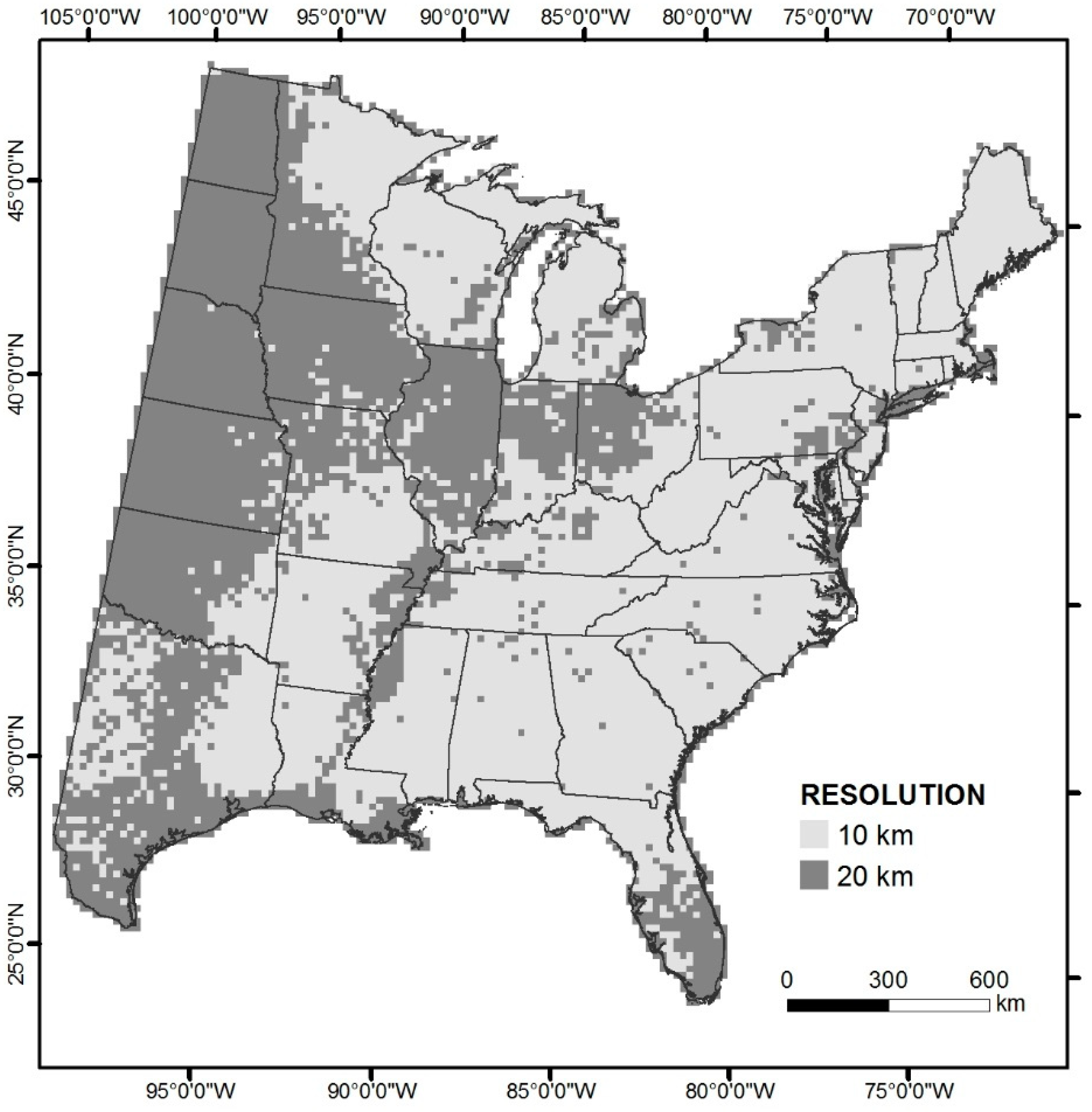
Tree Data. As done in the earlier effort [42], we used U.S. Forest Service Forest Inventory and Analysis (FIA, www.fia.fs.fed.us) data to derive individual tree species importance values (IV) for each of 84,204 FIA plots. All plots were included with no filtering. The assumption was if the species already grows there, it can grow there. The relative number of stems and relative basal area for each species were weighted equally to calculate IV for each plot. Thus, some species with large numbers of smaller stems (e.g., Ulmus, Acer, Fraxinus spp.) may be calculated as more important than species with fewer, but larger stems (e.g., some Quercus). All 84,204 annualized FIA records sampled during the period 2000–2016 were processed, and aggregated to cells with native resolutions of either 10 × 10 km or 20 × 20 km to represent the mean IV within the grid cell. We strove to increase spatial resolution, over that of our previous effort, where the FIA data would support it; to that end, a hybrid lattice was generated through an iterative algorithm to determine whether resolution could be increased to 10 × 10 km (four cells within each 20 × 20 km cell), or maintained at 20 × 20 km. To do so, a 10-km was accepted if ≥50% of the four 10-km cells within a 20-km cell contained two or more FIA plots, otherwise the focal 20-km cell was retained. The resulting hybrid lattice for the eastern U.S. had 29,357 cells, 84.7% of which were comprised of 10 × 10 km cells, and accounting for 2.49 million km2, or 58% of the eastern U.S. (Figure 2). The 20 × 20 km cells occupied 1.79 million km2, or 42% of the area, and were mostly confined to highly agricultural areas, predominantly in the western portion of the eastern U.S. (Figure 2). To minimize species that have too few samples to build a respectable model, species were only included if they had at least 60 grid cells with at least two FIA plots per cell. This filter resulted in a total of 125 species in the analysis.
Environmental Data. A suite of 45 environmental variables was used to predict IV, for 125 species across the entire eastern US. We used seven climate-related variables, seven elevation-related variables, a solar-related variation of day length variable, nine soil taxonomic orders, and 21 variables related to soil properties to derive the Random Forest models [41] predicting current species IV (Table 2). These data were acquired from various sources, with most soils information from gSURRGO [52], elevation data from the shuttle radar topography mission [63], a model of solar radiation via latitude [64], and a model of soil productivity based on soil taxonomy [65]. We then swapped the seven climate-related variables with future (2070–2099) projections of the same variables according to each of the six GCM/RCP combinations (see above), and Random Forest predicted future IVs for each species. It is important to note that we are not using elevation variables as a proxy for climate—we use them to discriminate among species that prefer lower elevation habitats (for example along the coastal plains or swamps) from those that prefer more elevated habitats with rugged terrain. Also, in addition to improving model fit, the numerous soil variables help restrain the models’ response under future climates and distinguish among species that are mostly climate driven vs. those that are less so.
2.2. Modeling
Individual tree species IV were modeled using the randomForest library [67] in R version 3.1.1 [68] (hereafter RF), in which 1001 regression trees were trained with eight randomly selected environmental variables evaluated at each node, and grown to include a minimum of 10 observations. To train the models, only grid cells within the hybrid lattice (10 × 10 or 20 × 20 km) were used that had (1) two or more FIA plots (to ensure representation within each cell), (2) ≥5% forest cover defined by the 2006 NLCD [69] (classes 41, 42, 43, and 90, to exclude very highly agricultural regions), and (3) a mean IV ≤ 1.5 times the inter-quartile range of IVs across all cells (to exclude outliers because they were unlikely to represent the full 100 or 400 km2). Each of the 1001 regression trees built by RF provides information about the predicted IV, and the default is to report the mean prediction. However, the random resampling of only eight of 45 variables at each node can result in spurious outcomes due to, for example, omission of an entire class of variables (e.g., climate); while these spurious trees rarely influence overall prediction [70], outliers can influence prediction distributions at a given cell [71]. Therefore, we compared the mean predicted value to the median for each cell; if the median = 0 and among all 1001 predicted values the coefficient of variation ≥2.75, then 0 was used as the predicted IV rather than the mean; which was 0 < IVmean < 8 among all species. This “mean-median” combination is a modification to the approach suggested by Roy and Larocque [71] which limits the influence on outlier predictions, minimizing the area of modeled low suitability, due to a few outliers within the 1001 regression trees for each species.
Once the RF model was trained, predictions of IV were made to all 29,357 cells irrespective of cell size within the hybrid lattice, whether or not at least 2 FIA plots were present, or whether percent forest cover was less or more than five percent.
2.3. Model Reliability
We created a model reliability (ModRel) score from a series of five metrics obtained from the performance statistics of each of 125 species. These included (1) a pseudo R2 obtained from the RF model (RF R2); (2) a Fuzzy Kappa (FK) metric which compares outputs of the imputed RF-predicted map to the FIA-derived map [72]; (3) the deviance of the CV (CVdev) among 30 regression trees via bagging [41]; and (4) the stability of the top five variables (Top5) from 30 regression trees, and (5) a true skill statistic (TSS) of the imputed RF. The first four were used previously, described in Iverson et al. [42]. The five variables were normalized to a 0–1 scale and weighted as follows to arrive at a final ModRel score: 0.33 × RF R2 + 0.33 × FK + 0.11 × CVdev + 0.11 × Top5 + 0.11 × TSS which gives more weighting to RF R2 and FK, a primary performance metric and a comparison of predicted to observed values, respectively. Then, ModRel scores were assigned to one of four classes: High (ModRel ≥ 0.7), medium (0.7 > ModRel > 0.54), low (0.55 > ModRel ≥ 0.14), and unreliable and excluded from further modeling (ModRel < 0.14).
2.4. Variable Importance
Each of the 45 predictor variables was scored for all species cumulatively according to a variable importance index, which was the average of three normalized (0–100) scores. First, the variable importance, as calculated within the RF function (percent increase in MSE based original and permuted predictors of the out-of-bag data—see the help for “importance” in randomForest library in R), for each of 125 species was summed. Second, the sum of the reciprocal of ranked predictor importance across all species was calculated; the reciprocal produced higher scores for top ranked variables. Third, the frequency, or count, of the number of times a predictor ranks in the top 10 across all species was tabulated. These metrics allowed comparison among the 45 variables for their value in creating the tree species models. Importantly, these metrics are based on all species across the entire eastern U.S. so that species that have specific requirements will not garner much support with these indicator metrics.
2.5. Area-Weighted Importance Values
To incorporate both the area and the relative abundance of each species, we calculated area-weighted importance values for each species. We use area-weighted importance values as a surrogate for the strength of suitable habitat across a species’ distribution. The higher the IV score, the higher the tendency for that species to occupy that cell, and the higher the possible basal area of that species within the cell. This measure of suitable habitat is not a probability of occurrence (though likely similar for many species) but rather an indication of the potential of the cell to host the species. Any value above 0 can be considered suitable habitat, though the strength of that habitat varies according to the area-weighted IV score. These values thus provide an estimate of each species’ importance based on the IV modeled for each cell (or partial cell), multiplied by the area the cell represents. Because of the variation of grid sizes (100 km2 or 400 km2), due to the hybrid grid structure, and the partial cells especially along coasts, the area-weighted values are truer to their actual and projected future suitable habitat. The ratio of future to present modeled condition represents the potential change of suitable habitat in the future, where values >1 indicate an increase in area-weighted importance and values <1 indicate a decrease.
2.6. Changes in Mean Center of Spatial Data
Within ArcGIS 10.3 (ESRI, Redlands, CA, USA), the Mean Center and Directional Distribution functions were used to calculate the current and future ‘center of gravity’ and directional ellipse within 1 standard deviation, respectively, of species ranges generated by our models. No weighting was applied to the IV, but only cells modeled to have an IV > 0 were considered in the calculation of the mean centers and directional ellipses. The coordinates of the mean center were used to calculate distance and direction of potential movement of the suitable habitat for each species and were visualized using polar graphs to evaluate potential changes among all species for each scenario of climate change.
2.7. Analysis of Dominants, Gainers, and Losers
The area-weighted IV allowed comparison of species prominence and potential change according to the climate scenarios, by spatial domain. These provide valuable supplements to FIA data and state reports (www.fia.fs.fed.us) on the current situation for tree species, as the IVs are based on both density (number of stems) and dominance (basal area) simultaneously. We provide this information for each of 37 states and the District of Columbia, and for five regions within the eastern US. Notably, for the six states split by the 100th meridian (our boundary of the eastern U.S.), some forest patches will be missed but the area in those states west of the 100th meridian is dominated by nonforest or western species (not modeled), with the exception of the Black Hills of South Dakota. We ranked each species according to the modeled current IV and selected the top three for each spatial unit and then calculated the potential changes in area-weighted IV, as ratios of future to current IVs, among the various scenarios of climate change.
2.8. Species-Level Maps
Maps representing species (abundance and suitable habitat under various scenarios) were generated for each species. Specifically, the maps show outputs of the (1) FIA estimate of current abundance, (2) modeled current distribution, and the future distributions according to the (3) CCSM45, (4) CCSM85, (5) GFDL45, (6) GFDL85, (7) Had45, (8) Had85, (9) mean of all three RCP4.5, and (10) mean of all three RCP8.5 scenarios.
2.9. Comparison to Earlier DISTRIB Models
We have been modeling tree species suitable habitat within the eastern U.S. since 1998 [17,39,40,42,43], and there have been changes in many dimensions throughout this period. First, we modeled 80 species at the county level of resolution, then 134 species at 20 × 20 km resolution, and most recently 125 species at a hybrid of 10 × 10 and 20 × 20 km resolution, depending on the density of FIA plots (~forest cover). Throughout the period, there has also been a remarkable improvement in environmental data, especially climate and soils data. And, the modeling improvement from regression tree analysis to random forests [41] was particularly dramatic in enhancing model performance. As expected when using multiple models, updated data sets, or variations in modelling technique, model outcomes will differ between iterations; this is true in this case too.
2.10. Scope and Limitations
The models depicted here represent changes in potentially suitable habitat according to scenarios of climate change; they do not depict projections of actual future distributions by 2100. Earlier work has shown that natural migration proceeds at a much slower pace than change in habitat, especially for long-lived trees [17,73,74,75]. Therefore, our projections of an increase in the range are likely to overestimate the actual distributions by century’s end, unless humans get seriously involved in moving species.
Though Random Forest has been shown to be a robust modeling tool, highly resistant to overfitting, we sometimes are making predictions into novel parameter space through extrapolation; nonetheless, the resistance to overfitting of Random Forest predictions gives us confidence that the extrapolations are suitably constrained and are not exaggerated projections [41]. Obviously, not all 125 species models are created equal, and we calculate several metrics to assess model reliability for each species [42].
When we model potential changes in suitable habitat, one would normally expect the greatest impacts to be experienced by young plants at the point of regeneration, when seedlings or saplings are more susceptible to the increased extreme weather events and other ramifications of the changing climate. However, mature forests are certainly also susceptible, either directly via droughts, especially ‘hot’ droughts [76], or indirectly via pests and pathogens [77]. Because the models are based on FIA inventories of trees >2.5 cm dbh, the regeneration component is not well represented in the model formulations. We are modeling the potential niche space that may be available to species under future climates, which may not be the realized niche because disturbances and extreme events will be operating within the suitable habitats. Though the FIA data, in effect, integrates past disturbances by documenting those species that have survived past events, we cannot anticipate future disturbances (like an exotic pest invasion) that will influence actual future distribution and abundance. Further, we cannot assume that all species are in equilibrium with their current climate or other environmental variables.
3. Results and Discussion
3.1. Model Reliability and Variable Importance
Of the 125 species in this assessment, we scored 29 species with high model reliability, 47 with medium, and 49 with lower model reliability. These model reliability classes are presented for each species in Table A1. Admittedly, the cut off values presented in the methods section are arbitrary and adjusting the cut offs would change the proportion of each model reliability class. We chose to stay conservative in assigning the cut offs, leading to a loading of species at the lower end of reliability.
When we scored each of the 45 predictor variables according to a variable importance index, we found the climate variables dominated in importance. In fact, seven of the top nine variables were the climate variables. Of course, several of these variables are correlated with each other across the entire eastern U.S. but will be important locally for particular species. The first and second ranked variables were summer (30-year mean of the warmest month) and winter (30-year mean of the coldest month) temperatures; these indicate some species are limited by cold, some are linked to warm temperatures, and some may be driven by both together. Because these metrics are based on all species across the entire eastern U.S., the wide ranging, generalist species will tend to be correlated with wide ranging temperature or precipitation patterns as well. The day length coefficient of variation among months (based on latitude) was the most influential non-climate variable, followed by soil variables pH, texture (soil fraction passing a sieve with a 2 mm square opening), soil productivity (based on soil taxonomic family), and permeability (saturated hydraulic conductivity). The lower ranked variables, though not rated high for all species together, will rank high for individual species in particular habitats, etc. Though space prevents discussion of individual species and their variables of importance, these will be presented in upcoming updates to our Climate Change Tree Atlas (www.fs.fed.us/nrs/atlas).
3.2. Potential Changes in Species Area-weighted Importance Values
For the 125 species with acceptable models, Table 3 provides an indication of the quantity of species that may lose (Future: Current ratios < 0.9) or gain (ratios > 1.1) suitable habitat by 2100, as well as those projected to remain somewhat stable (0.9 < ratios < 1.1). Averaged across all scenarios, 88 species showed at least a 10% increase in area-weighted IV, and 26 species showed at least a 10% decrease, with 12 species having little or no change (Table 3). For those 88 species inclined to have increasing habitat, the RCP8.5 scenario showed more species at least doubling habitat (55 species) than under the RCP4.5 scenario (42 species) of lower emissions. Notably, there was not much difference between RCPs for those species losing habitat (Table 3). Species included among those projected to lose substantial habitat are: Acer nigrum Michx. f. (black maple), A. spicatum Lam. (mountain maple), Picea mariana (black spruce), Populus balsamifera L. (balsam poplar), Prunus pensylvanica L.f. (pin cherry), and Sorbus americana Marshall (American mountain-ash) (Table A1). Among those species showing substantial increases in suitable habitat are: Carpinus caroliniana Walter (American hornbeam), Celtis laevigata Willdenow (sugarberry), Magnolia grandiflora L. (southern magnolia), Ostrya virginiana (Mill.) K.Koch (eastern hophornbeam), Pinus echinata Mill. (shortleaf pine), P. palustris Mill. (longleaf pine), Quercus falcata Michx. (southern red oak), Quercus marilandica Muenchh. (blackjack oak), Quercus michauxii Nutt. (swamp chestnut oak), Q. nigra (water oak), Q. phellos (willow oak), Quercus phellos L. (post oak), Quercus phellos L. (live oak), Taxodium distichum (L.) Rich. (bald cypress), and Ulmus alata Michx. (winged elm) (Table A1).
The data do show that for many of the species gaining in excess of 10% in habitat, they are often from less reliably modeled species than those species losing habitat. For example, only 12 of 88 species (14%) which show at least 10% increase in habitat had highly reliable models, but 12 of 26 species (46%) showing a decrease of at least 10% had highly reliable models (Table A1). For those more common species (arbitrarily selected as those with the sum of IV > 15,000), those ratios are 11 of 34 (32%) for gainers compared to 8 of 8 (100%) for the losers. The large gainers fall into three categories: First, the species is currently common in a region that is now quite warm and fairly dry, that being the southwestern portion of the eastern U.S. (e.g., Texas, Oklahoma, southern Missouri). These species, like Quercus stellata (post oak), Quercus marilandica Muenchh. (blackjack oak), Carya texana Buckley (1861) (black hickory), ashe juniper (Juniperus ashei J. Buchholz) and Juniperus virginiana L. (eastern red cedar), are primarily temperature driven, and expand greatly in suitable habitat when provided much warmer temperatures as projected under climate change. Second, the species is currently quite rare or sparse according to current FIA plot data, and the models project the species to ‘fill in’ some additional territory with suitable habitat. Species in this category include Diospyros virginiana L. (common persimmon), Ilex opaca Aiton (American holly), and Ostrya virginiana (Mill.) K.Koch (eastern hophornbeam). Third, the species is an important southern species now but is expected to substantially expand its suitable habitat northward by end of the century. These species include Quercus falcata (southern red oak), Quercus nigra L. (water oak), Pinus echinata (shortleaf pine), and P. palustris (longleaf pine) (Table A1).
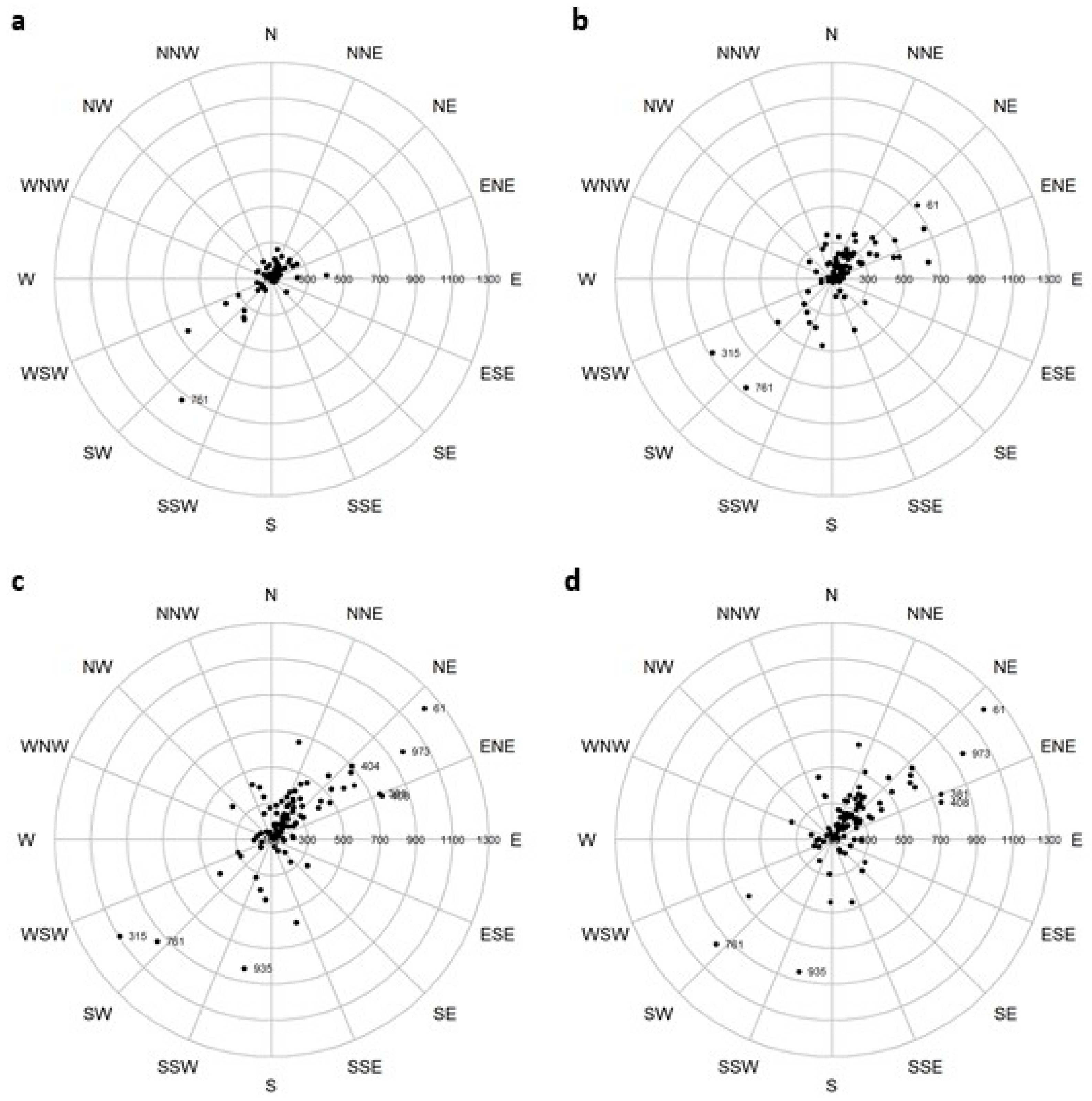
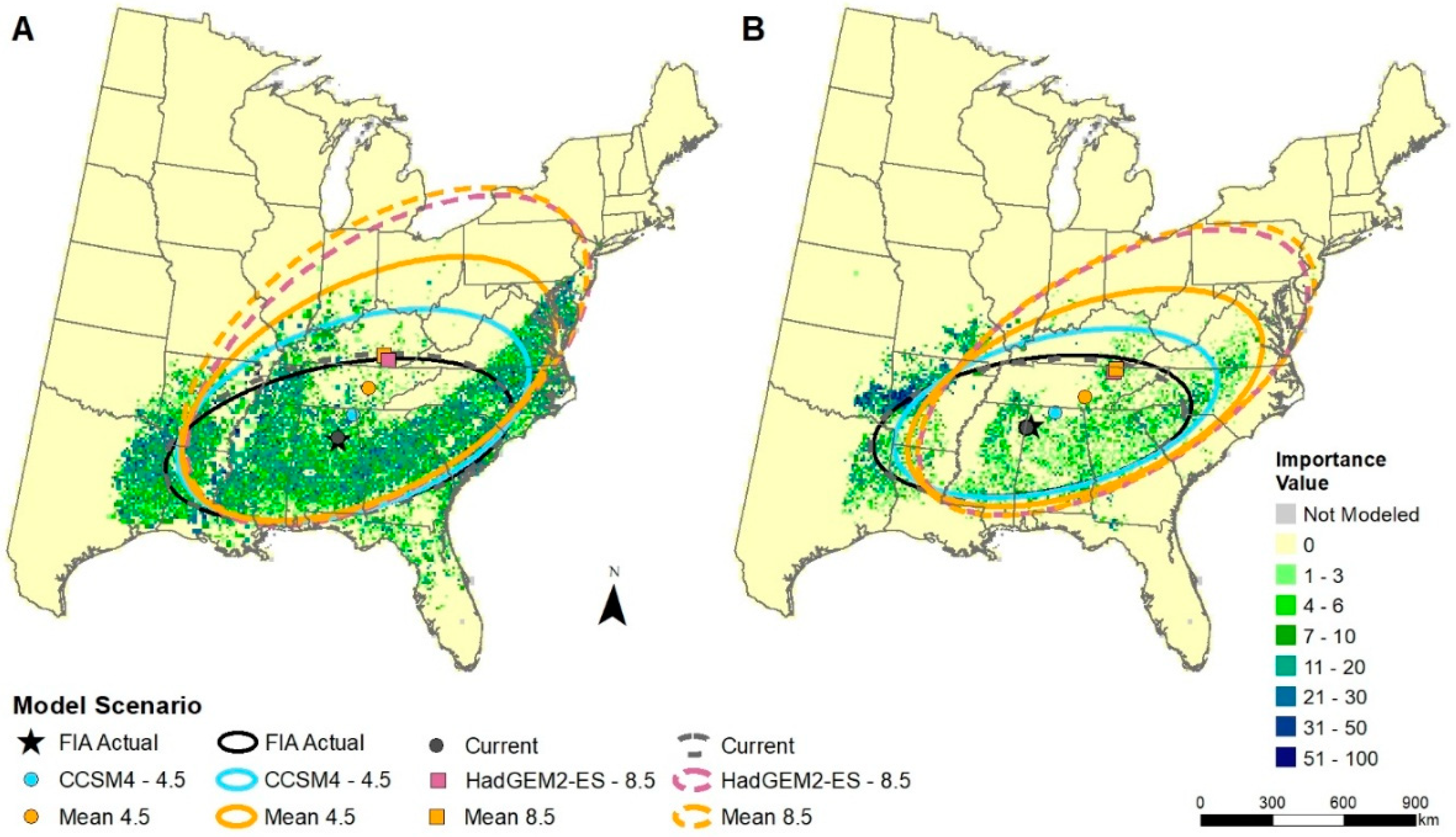
3.3. Changes in Mean Center of Spatial Data
The potential changes in mean centers of suitable habitat under various scenarios of climate change indicate that roughly 3–4 times as many species show habitat movement in a northerly direction as compared to a southerly direction (Table 4, Figure 3). As many as 81 species (RCP8.5 mean) could have mean center movement at least 100 km northward. The data also clearly show that those northward-moving species will likely have their mean habitat centers move greater distances under the hotter (RCP8.5) scenarios as compared to the RCP4.5 scenarios. Some of the species modeled to move habitats long distances northward include Carya texana (black hickory), Quercus virginiana (live oak), and Ulmus crassifolia (winged elm) (Figure 3). The scenario with the least change in temperature, CCSM45, also shows less northward movement of mean centers, but this scenario still has 54 species moving habitats at least 100 km by the end of the century. Some of the species moving habitats southward include Acer pensylvanicum L. (striped maple), Prunus pensylvanica (pin cherry), and Sorbus americana (American mountain ash) (Figure 3); these species models, however, had lower model reliability and are complicated by the geographic influence of the spine of the Appalachian Mountains. Example maps showing the mean centers and their ellipses around current and potential future habitat distributions for two southern species, Liquidambar styraciflua L. and Pinus echinata, are shown in Figure 4. Fei et al. [78], in an analysis of FIA data across three decades for 86 species/groups in the eastern U.S., found that 62% of species show evidence for a northward shift and that 73% of species show evidence for a westward shift. This westward trend was associated with changes in moisture availability (more moisture now westward) and successional trends (afforestation farther west), though the much sparser FIA data westward into the highly agricultural Midwestern Corn Belt can also contribute to the differences in results with ours. Of the species we have in common (n = 78) with the Fei et al. study, our results from the GCM85 scenario show much more potential for northward (87% N, 13% S) over westward (31% W, 69% E) migration of climatically suitable habitat. In future, the GCMs do show a lot more warming northward as compared to the previous 30 years [78,79], and when coupled with a probable constraint of the increased moisture westward [79], these two studies are not incongruent.
Numbers represent the FIA species codes for a few species with potential long distance movements (shown in km): 61 = Juniperus ashei J. Buchholz, 315 = Acer pensylvanicum L., 404 = Carya illinoensis (Wangenh.) K.Koch, 408 = Carya texana Buckley, 761 = Prunus pensylvanica L.f., 935 = Sorbus americana, 973 = Ulmus crassifolia.
3.4. Analysis of Dominants, Gainers, and Losers by State and Region
In this analysis we identified, for the entire East, five regions, and 37 states plus the District of Columbia, the dominant three species now and what their overall changes are projected for suitable habitat, with 1 meaning no change, <1 meaning a loss in habitat, and >1 meaning a gain in habitat (Table 5). Over the entire eastern U.S., the top three species currently are loblolly pine (Pinus taeda), red maple (Acer rubrum), and sweetgum (Liquidambar stryraciflua L.). Of the 36 unique species ranked among the top three positions, those that most frequently scored among the dominant three species are red maple (for 21 of 44 states or regions), loblolly pine (15 of 44), sugar maple (Acer saccharum, 11 of 44), and sweetgum (10 of 44) (Table 5). By genus, the three Acer species were found among the top three species 33 times, the five Pinus species 25 times, and the nine Quercus species 23 times.
For the top three species within the 38 state (and District of Columbia) rankings (n = 114), 50 (44%) are expected to lose >10% of their suitable habitat, while 41 (36%) species are projected to gain >10% of habitat by 2100 for the RCP 4.5 scenario; comparable numbers under RCP 8.5 are 58 (51%) losers and 40 (35%) gainers. So, although more of these dominant species are expected to lose habitat suitability in the changed climate, the fact that they are abundant presently and often very adaptable to a changing climate [80,81] increases the probability that many of these species, even the losers, may still be plentiful in their respective states by 2100.
Contrary to the data for the entire suite of 125 species, where 88 species were modeled to gain at least 10% habitat (Table 3), the analysis of only the top three species by state or region shows that a larger number of species are projected to lose habitat as compared to gain habitat (Table 5). Of the 132 iterations of species listed on Table 5 under regions or states, 56 species lost >10% habitat and 51 gained >10% habitat. Primary losers were Acer rubrum, A. saccharum, Liriodendron tulipifera L., and Populus tremuloides, while primary gainers were Pinus taeda and Liquidambar styraciflua.
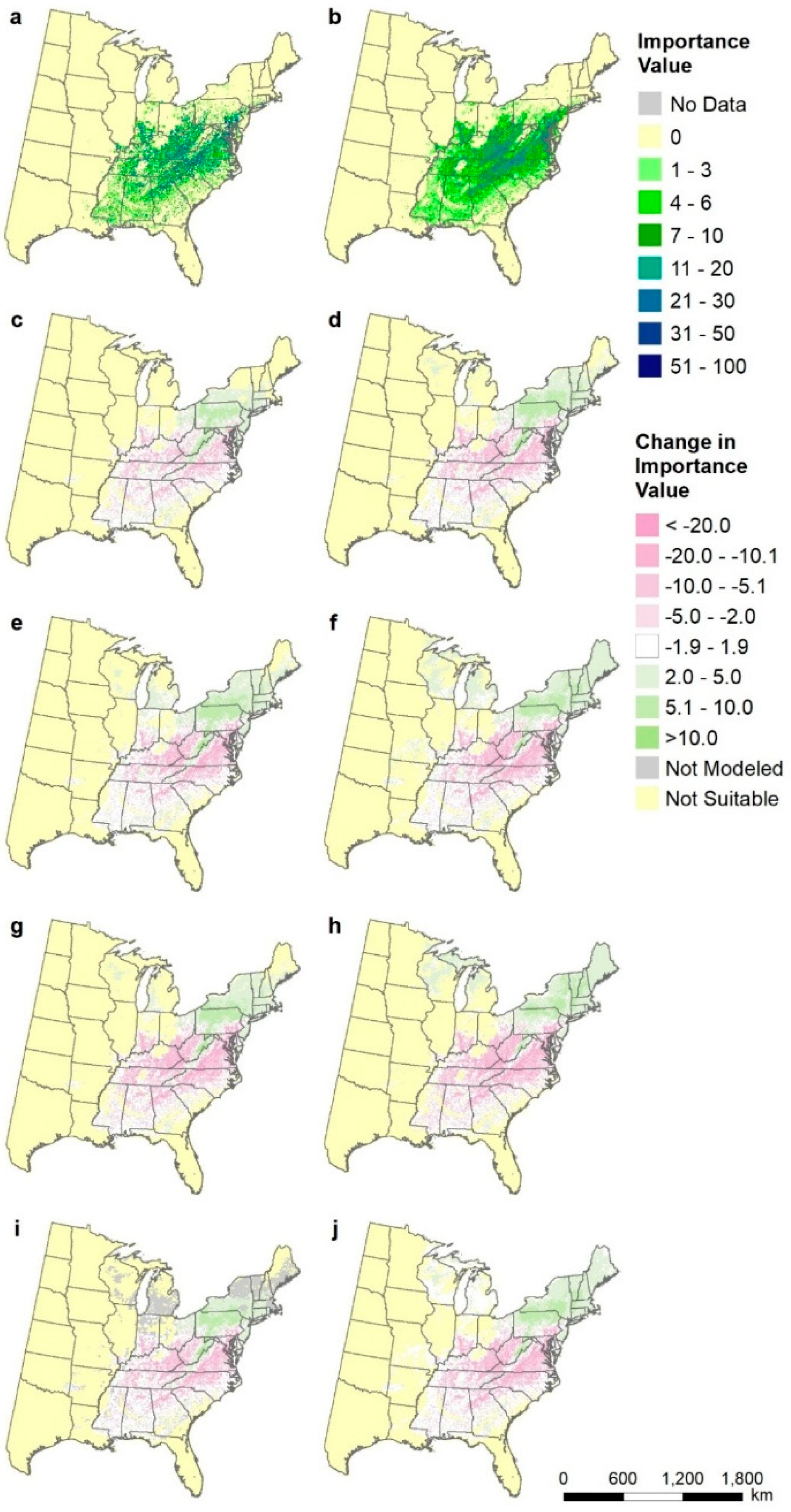
3.5. Species-Level Maps
Though putting 10 maps on a page masks fine-scale visualization, it does provide a way to assess the current distribution according to the relatively sparse FIA plots, the modeled current distribution, and the potential future distributions according to each of the model/RCP scenarios, as well as the mean RCP 4.5 and 8.5. For example, Liriodendron tulipifera (yellow poplar), a species important for wood products throughout its range (Figure 5) shows a general northward expansion of suitable habitat under warming, with more expansion under RCP8.5 vs. RCP4. The least expansion is with the relatively cool CCSM4 model as compared to the more equivalent Hadley and GFDL models. However, with the driest Hadley model (either RCP4.5 or RCP8.5), habitat for yellow poplar noticeably contracts in the southern third of its current distribution (Figure 5). These maps are available in Figure A1, Figure A2 and Figure A3 for three other species, Pinus echinata (shortleaf pine) P. teada (loblolly pine), and Liquidambar styraciflua (sweetgum); all species will eventually be on our atlas website www.fs.fed.us/nrs/atlas.
3.6. Comparison to Earlier DISTRIB Models
As expected, there are differences between DISTRIB-II outputs described here from those presented in our earlier work [15]. In our current effort, differences mainly arise from using a hybrid lattice approach, and also from: (1) Newer FIA records, (2) recent 30-year climate normals, (3) a newer set of predictor variables, (4) removal of outlier training data, and (5) modifying predicted IVs with the mean-median combination. The recent FIA records provide information about disturbances and changes in species demographics, while the 30-year climate normals attempt to match conditions experienced by the trees inventoried by FIA. The newer set of environmental predictors incorporates finer scale information (e.g., gSSURGO soils), as well as additional variables not previously used. The removal of outliers from training datasets aims to limit the influence of unrepresentative cells that might result from plantations or severe disturbance events, while the modification of predicted values with the mean-median combination reduced the influence of spurious predictions among the prediction set.
Attributing the differences in results between DISTRIB and DISTRIB-II to any single or combination of the listed factors would be very difficult to quantify and of little practical value to forest managers. Suffice it to say that the newer results are an improvement over the earlier ones. However, as with our earlier results, models with low reliability should be interpreted with caution. As always with modeling studies, ‘all models are wrong’ [82]; we strive to make them useful by making them available to use in concert with any other information and experience available to the decision makers.
4. Conclusions
The forests of the eastern United States are characterized by a diverse assemblage of tree species. Climate change has the potential to shift and influence species patterns, thereby creating novel communities, with the greatest disruption and change clearly linked to the emissions pathways that unfold over the course of this century. By quantifying potential habitat changes across a wide array of species over a broad geographic extent, we can consider several dimensions of potential habitat change that lend to understanding individual species responses, as well as focused regional quantification that lend to informed on-the-ground adaptation planning. The trend of increasing general habitat conditions for a large portion of the species is a function of spreading at the range margin extents with, in many cases, a decline in core habitat suitability. Those species projecting losses, while fewer in number, generally show a contraction in the range of suitable habitat under either RCP, but especially so under RCP 8.5. In many cases, a finer extent of regions or state level evaluations reveals the potential impact of shifting habitats via ranked species importance and summary of winners and losers by states or regions. In these more discrete extents, the gradual fading in or out for species presents useful information for planners. Many of the current top species projected to decline in the region (even though their range-wide ratio may be increasing) epitomize the conditions where macro level pressures of climate change can have local level implications. In the end, these results show the high potential for a reshuffling of where suitable habitats for species will occur across the eastern United States, and it is clear that these will reshape competitive pressures and ultimate final outcomes that are beyond any modeling approach. Therefore, we intend these models to be one piece of a package of information that practitioners use for decisions related to adapting to the changing climate we now face. Working together, adaptations in silviculture and ecological management should improve the potential for eastern U.S. forests to continue to thrive in the coming decades.
Author Contributions
All four authors cooperated on conceptualization, methodology, validation, formal analysis, investigation, data curation, visualization, review and editing, and preparing the proposal for funding. L.R.I. prepared the original draft, and supervised and administered the overall project.
Funding
This research was funded by the USDA Forest Service, Northern Research Station, the Northern Institute of Applied Climate Science, and the USDA Climate Hubs as part of their appropriated funding.
Acknowledgments
Climate scenarios used were from the NEX-DCP30 dataset, prepared by the Climate Analytics Group and NASA Ames Research Center using the NASA Earth Exchange, and distributed by the NASA Center for Climate Simulation (NCCS). We appreciate reviews by Bryce Adams, Patricia Leopold, and Chris Swanston, along with the editors and reviewers of this Forests issue.
Conflicts of Interest
The authors declare no conflict of interest The funders had no role in the design of the study; in the collection, analyses, or interpretation of data; in the writing of the manuscript, or in the decision to publish the results.
Appendix A

Table A1.
Importance value × area scores (FIAsumIV) and their future:current ratios showing potential gains (light green 1.1–2.0, dark green > 2.0-fold increase) or losses (orange 0.5–0.9, red < 0.5 times decrease) or no change (black 0.9–1.1) under three scenarios of climate change: CCSM4.5, GFDL8.5, Had8.5 and mean of the three models for each RCP (GCM45 and GCM85). Also shown is overall average score (GCMave), and the model reliability for each species.
| Scientific Name | Model Reliability | FIA sumIV | CCSM45 | GFDL85 | HAD85 | GCM45 | GCM85 | GCMave |
|---|---|---|---|---|---|---|---|---|
| Abies balsamea (L.) Mill. | High | 35,606 | 0.496 | 0.504 | 0.492 | 0.495 | 0.506 | 0.500 |
| Acer barbatus Michx. | Low | 1729 | 1.758 | 5.877 | 5.654 | 3.026 | 5.277 | 3.631 |
| Acer negundo L. | Low | 25,259 | 1.356 | 2.096 | 1.887 | 1.637 | 1.889 | 1.763 |
| Acer nigrum L. | Low | 678 | 0.409 | 0.292 | 0.282 | 0.364 | 0.299 | 0.340 |
| Acer pensylvanicum L. | Medium | 2549 | 0.752 | 0.565 | 0.547 | 0.672 | 0.580 | 0.653 |
| Acer rubrum L. | High | 165,591 | 1.030 | 0.915 | 0.871 | 0.993 | 0.920 | 0.956 |
| Acer saccharinum L. | Low | 14,872 | 1.804 | 3.044 | 2.445 | 2.309 | 2.630 | 2.203 |
| Acer saccharum Marshall | High | 88,010 | 0.945 | 0.906 | 0.819 | 0.932 | 0.880 | 0.906 |
| Acer spicatum Lam. | Low | 472 | 0.214 | 0.177 | 0.171 | 0.177 | 0.164 | 0.220 |
| Aesculus flava Sol. | Low | 1682 | 0.895 | 0.666 | 0.564 | 0.775 | 0.682 | 0.705 |
| Aesculus glabra Willd. | Low | 999 | 0.720 | 0.588 | 0.572 | 0.640 | 0.584 | 0.603 |
| Amelanchier spp. | Low | 2558 | 0.956 | 1.278 | 1.250 | 1.024 | 1.181 | 1.015 |
| Asimina triloba (L.) Dunal | Low | 738 | 0.488 | 0.519 | 0.518 | 0.495 | 0.497 | 0.481 |
| Betula alleghaniensis Britt. | High | 17,123 | 0.828 | 0.635 | 0.634 | 0.753 | 0.654 | 0.703 |
| Betula lenta L. | High | 13,368 | 1.029 | 0.806 | 0.802 | 0.966 | 0.844 | 0.909 |
| Betula nigra L. | Low | 3988 | 1.632 | 6.922 | 8.275 | 4.053 | 6.875 | 4.749 |
| Betula papyrifera Marshall | High | 21,096 | 0.940 | 0.833 | 0.779 | 0.918 | 0.834 | 0.876 |
| Betula populifolia Marsh. | Low | 1622 | 1.045 | 1.293 | 1.157 | 1.154 | 1.191 | 1.095 |
| Carpinus caroliniana Walter | Low | 9337 | 2.417 | 4.278 | 3.472 | 2.913 | 3.756 | 2.954 |
| Carya alba Sarg. | Medium | 22,233 | 1.831 | 2.998 | 3.185 | 2.267 | 2.920 | 2.593 |
| Carya aquatica (F.Michx.) Nutt. | Medium | 2624 | 1.278 | 1.619 | 1.699 | 1.380 | 1.641 | 1.393 |
| Carya cordiformis (Wangenh.) K.Koch | Low | 12,853 | 1.468 | 2.757 | 2.284 | 1.859 | 2.315 | 1.882 |
| Carya glabra Miller | Medium | 22,303 | 1.240 | 1.494 | 1.318 | 1.280 | 1.401 | 1.341 |
| Carya illinoinensis (Wangenh.) K.Koch | Low | 6698 | 2.613 | 13.336 | 15.386 | 5.479 | 12.017 | 7.580 |
| Carya laciniosa (Mill.) K.Koch | Low | 1009 | 1.051 | 1.767 | 1.080 | 1.241 | 1.340 | 1.177 |
| Carya ovate (Mill.) K.Koch | Medium | 19,547 | 1.149 | 1.356 | 1.170 | 1.281 | 1.262 | 1.271 |
| Carya texana Buckley (1861) | High | 9390 | 2.126 | 6.676 | 7.545 | 3.686 | 6.198 | 4.358 |
| Celtis laevigata Willdenow | Medium | 16,556 | 2.469 | 6.786 | 7.940 | 3.893 | 6.580 | 5.236 |
| Celtis occidentalis L. | Medium | 21,798 | 1.516 | 2.420 | 1.974 | 1.861 | 2.076 | 1.968 |
| Cercis Canadensis L. | Low | 4198 | 1.419 | 3.579 | 3.607 | 2.118 | 3.189 | 2.353 |
| Chamaecyparis thyoides (L.) B.S.P. | Low | 821 | 1.464 | 1.927 | 0.697 | 1.704 | 1.542 | 1.475 |
| Cornus florida L. | Medium | 10,589 | 1.545 | 1.868 | 1.631 | 1.607 | 1.765 | 1.554 |
| Diospyros virginiana L. | Low | 7074 | 1.981 | 8.115 | 8.345 | 4.039 | 7.027 | 4.814 |
| Fagus grandifolia Ehrh. | High | 35,486 | 1.118 | 1.291 | 0.996 | 1.163 | 1.193 | 1.178 |
| Fraxinus Americana L. | Medium | 42,548 | 1.314 | 1.633 | 1.547 | 1.455 | 1.559 | 1.507 |
| Fraxinus nigra Marshall | Medium | 13,276 | 1.114 | 0.934 | 0.890 | 1.080 | 0.955 | 0.997 |
| Fraxinus pennsylvanica Marshall | Low | 47,622 | 1.872 | 2.747 | 2.738 | 2.200 | 2.627 | 2.413 |
| Fraxinus quadrangulata Michx. | Low | 631 | 0.870 | 1.045 | 0.709 | 0.888 | 0.889 | 0.827 |
| Gleditsia triacanthos L. | Low | 11,912 | 1.317 | 3.096 | 3.083 | 1.907 | 2.739 | 2.078 |
| Gordonia lasianthus (L.) Ellis | Medium | 2418 | 1.666 | 1.812 | 1.567 | 1.651 | 1.712 | 1.549 |
| Halesia spp. | Low | 150 | 1.354 | 1.627 | 1.314 | 1.486 | 1.518 | 1.391 |
| Ilex opaca Aiton | Medium | 5391 | 1.829 | 2.456 | 2.165 | 2.018 | 2.304 | 1.956 |
| Juglans nigra L. | Low | 24,037 | 1.282 | 2.367 | 2.081 | 1.678 | 2.069 | 1.873 |
| Juniperus ashei J. Buchholz | High | 21,113 | 1.334 | 3.632 | 7.938 | 1.863 | 4.673 | 3.268 |
| Juniperus virginiana L. | Medium | 49,834 | 1.794 | 3.717 | 3.864 | 2.524 | 3.508 | 3.016 |
| Larix laricina (Du Roi) K. Koch | High | 12,797 | 1.198 | 1.170 | 1.161 | 1.238 | 1.215 | 1.176 |
| Liquidambar styraciflua L. | High | 91,344 | 1.342 | 1.816 | 1.802 | 1.479 | 1.730 | 1.604 |
| Liriodendron tulipifera L. | High | 63,276 | 0.895 | 0.821 | 0.645 | 0.807 | 0.766 | 0.786 |
| Maclura pomifera (Raf.) Schneid. | Medium | 11,988 | 1.167 | 2.920 | 2.610 | 1.755 | 2.408 | 1.883 |
| Magnolia acuminata L. | Low | 1734 | 1.058 | 1.106 | 1.066 | 1.039 | 1.086 | 1.008 |
| Magnolia fraseri Walter | Low | 651 | 1.542 | 1.667 | 1.610 | 1.540 | 1.653 | 1.465 |
| Magnolia grandiflora L. | Low | 1407 | 5.634 | 11.214 | 3.819 | 6.490 | 8.227 | 6.387 |
| Magnolia macrophylla Michx. | Low | 292 | 0.891 | 0.979 | 0.678 | 0.879 | 0.889 | 0.823 |
| Magnolia virginiana L. | Medium | 7875 | 2.622 | 3.793 | 1.945 | 2.798 | 3.129 | 2.658 |
| Morus rubra L. | Low | 8905 | 1.432 | 3.160 | 1.991 | 1.955 | 2.345 | 1.904 |
| Nyssa aquatic L. | Medium | 5014 | 1.284 | 1.856 | 1.215 | 1.377 | 1.587 | 1.360 |
| Nyssa biflora Walter | Medium | 14,558 | 1.716 | 2.140 | 1.813 | 1.816 | 1.991 | 1.760 |
| Nyssa sylvatica Marshall | Medium | 25,962 | 1.772 | 2.576 | 2.449 | 2.037 | 2.450 | 2.243 |
| Ostrya virginiana (Mill.) K.Koch | Low | 12,225 | 2.107 | 3.507 | 2.670 | 2.599 | 3.017 | 2.500 |
| Oxydendrum arboretum (L.) DC. | High | 11,224 | 1.020 | 0.911 | 0.701 | 0.885 | 0.860 | 0.877 |
| Persea borbonia (L.) Spreng. | Low | 2757 | 1.729 | 2.491 | 1.563 | 1.839 | 2.078 | 1.776 |
| Picea glauca (Moench) Voss | Medium | 7764 | 0.758 | 0.844 | 0.863 | 0.778 | 0.842 | 0.807 |
| Picea mariana (Mill.) Britton, Sterns & Poggenburg | High | 14,500 | 0.497 | 0.468 | 0.453 | 0.474 | 0.460 | 0.534 |
| Picea rubens Sarg. | High | 13,049 | 0.689 | 0.556 | 0.554 | 0.612 | 0.555 | 0.637 |
| Pinus banksiana Lamb. | Medium | 9280 | 0.719 | 0.635 | 0.642 | 0.689 | 0.661 | 0.702 |
| Pinus clausa (Chapm. ex Engelm.) Sarg. | Medium | 3740 | 1.223 | 1.573 | 0.850 | 1.413 | 1.275 | 1.263 |
| Pinus echinata Mill. | High | 32,601 | 2.147 | 3.848 | 3.985 | 2.796 | 3.665 | 3.231 |
| Pinus elliottii Engelm. | High | 57,498 | 1.450 | 2.093 | 1.622 | 1.577 | 1.858 | 1.718 |
| Pinus glabra Walter | Low | 1039 | 0.507 | 0.608 | 0.297 | 0.551 | 0.487 | 0.533 |
| Pinus palustris Mill. | Medium | 19,920 | 2.677 | 4.428 | 2.167 | 2.933 | 3.507 | 3.220 |
| Pinus pungens Lamb. | Low | 527 | 0.798 | 1.297 | 1.541 | 1.061 | 1.246 | 1.061 |
| Pinus resinosa Sol. ex Aiton | Medium | 17,992 | 0.945 | 0.967 | 0.937 | 0.998 | 0.973 | 0.985 |
| Pinus rigida Mill. | High | 5653 | 0.754 | 0.948 | 0.982 | 0.818 | 0.928 | 0.854 |
| Pinus serotina Michx. | Medium | 4019 | 1.471 | 1.569 | 1.203 | 1.335 | 1.448 | 1.298 |
| Pinus strobus L. | High | 42,529 | 1.137 | 0.882 | 0.827 | 1.090 | 0.921 | 1.006 |
| Pinus taeda L. | High | 271,571 | 1.178 | 1.404 | 1.285 | 1.212 | 1.324 | 1.268 |
| Pinus virginiana Mill. | High | 21,514 | 0.915 | 0.933 | 0.888 | 0.843 | 0.913 | 0.878 |
| Planera aquatic J.F.Gmel. | Low | 932 | 1.940 | 3.579 | 4.961 | 2.526 | 3.987 | 2.854 |
| Platanus occidentalis L. | Low | 11,992 | 1.963 | 4.698 | 4.200 | 2.803 | 4.053 | 3.030 |
| Populus balsamifera L. | Medium | 5854 | 0.431 | 0.314 | 0.423 | 0.380 | 0.385 | 0.445 |
| Populus deltoids W.Bartram ex Marshall | Low | 11,742 | 1.935 | 4.570 | 3.983 | 2.881 | 4.034 | 3.034 |
| Populus grandidentata Michaux | Medium | 12,814 | 1.218 | 1.034 | 0.974 | 1.235 | 1.074 | 1.094 |
| Populus tremuloides Michx. | High | 54,642 | 0.814 | 0.671 | 0.636 | 0.775 | 0.691 | 0.733 |
| Prunus pensylvanica L.f. | Low | 1734 | 0.354 | 0.132 | 0.151 | 0.284 | 0.164 | 0.259 |
| Prunus serotina Ehr. | Medium | 60,388 | 1.380 | 1.529 | 1.404 | 1.477 | 1.466 | 1.472 |
| Quercus alba L. | Medium | 87,470 | 1.225 | 1.364 | 1.300 | 1.317 | 1.330 | 1.324 |
| Quercus bicolor Willd. | Low | 2188 | 1.833 | 3.550 | 2.420 | 2.713 | 3.077 | 2.549 |
| Quercus coccinea Muenchh. | Medium | 17,739 | 1.128 | 1.221 | 1.137 | 1.168 | 1.208 | 1.188 |
| Quercus ellipsoidalis E.J.Hill | Medium | 6120 | 1.679 | 1.915 | 1.454 | 1.909 | 1.733 | 1.677 |
| Quercus falcate Michx. | Medium | 24,747 | 2.091 | 3.581 | 4.291 | 2.697 | 3.659 | 3.178 |
| Quercus imbricaria Michx. | Medium | 4356 | 0.680 | 0.802 | 0.516 | 0.772 | 0.635 | 0.704 |
| Quercus incana Bartram | Low | 624 | 1.050 | 3.781 | 9.120 | 2.678 | 5.097 | 3.404 |
| Quercus laevis Walter | Medium | 2731 | 1.205 | 1.590 | 1.009 | 1.258 | 1.327 | 1.211 |
| Quercus laurifolia Michx. | Medium | 15,945 | 1.947 | 2.739 | 1.708 | 2.046 | 2.263 | 1.974 |
| Quercus lyrata Walter | Medium | 4159 | 1.589 | 3.426 | 3.826 | 2.166 | 3.289 | 2.435 |
| Quercus macrocarpa Michx. | Medium | 19,711 | 1.705 | 1.941 | 1.592 | 1.859 | 1.816 | 1.837 |
| Quercus marilandica Muenchh. | Medium | 10,061 | 2.750 | 10.400 | 11.679 | 5.241 | 9.588 | 6.459 |
| Quercus michauxii Nutt. | Low | 2156 | 2.111 | 3.834 | 2.445 | 2.643 | 3.098 | 2.531 |
| Quercus muehlenbergii Engelm. | Medium | 6459 | 1.230 | 2.054 | 1.388 | 1.484 | 1.613 | 1.433 |
| Quercus nigra L. | High | 46,637 | 2.089 | 3.282 | 3.325 | 2.568 | 3.195 | 2.882 |
| Quercus pagoda Raf. | Medium | 7681 | 2.027 | 3.388 | 3.255 | 2.470 | 3.199 | 2.539 |
| Quercus palustris Münchh. | Low | 4434 | 0.974 | 2.846 | 1.892 | 1.347 | 1.970 | 1.510 |
| Quercus phellos L. | Low | 10,282 | 2.116 | 3.299 | 3.727 | 2.625 | 3.336 | 2.653 |
| Quercus prinus Willd. | High | 34,675 | 1.186 | 1.270 | 1.177 | 1.191 | 1.233 | 1.212 |
| Quercus rubra L. | Medium | 55,330 | 1.410 | 1.460 | 1.337 | 1.478 | 1.416 | 1.447 |
| Quercus shumardii Buckland | Low | 2523 | 1.127 | 5.424 | 4.020 | 2.050 | 3.989 | 2.664 |
| Quercus stellate Wangenh. | High | 58,812 | 2.169 | 4.671 | 5.252 | 3.077 | 4.504 | 3.791 |
| Quercus texana Buckley | Low | 2363 | 1.282 | 1.681 | 1.597 | 1.361 | 1.589 | 1.353 |
| Quercus velutina Lam. | High | 44,550 | 1.598 | 2.469 | 2.301 | 1.962 | 2.273 | 2.118 |
| Quercus virginiana Mill. | High | 25,609 | 2.450 | 7.093 | 10.064 | 3.789 | 7.552 | 5.670 |
| Robinia pseudoacacia L. | Low | 18,414 | 1.380 | 3.449 | 3.471 | 1.922 | 3.030 | 2.476 |
| Sabal palmetto (Walt.) Lodd. | Medium | 4949 | 2.046 | 3.867 | 2.557 | 2.337 | 3.123 | 2.473 |
| Salix nigra Marshall | Low | 13,959 | 1.445 | 4.936 | 5.616 | 2.458 | 4.558 | 3.075 |
| Sassafras albidum (Nutt.) Nees | Low | 14,728 | 1.477 | 2.377 | 2.631 | 1.871 | 2.346 | 1.908 |
| Sideroxylon lanuginosum ssp. lanuginosum | Low | 2109 | 7.622 | 49.696 | 89.291 | 23.994 | 56.912 | 34.731 |
| Sorbus Americana Marshall | Low | 147 | 0.397 | 0.265 | 0.292 | 0.334 | 0.282 | 0.330 |
| Taxodium ascendens Brongn. | Medium | 8177 | 2.305 | 4.612 | 2.979 | 2.467 | 3.457 | 2.646 |
| Taxodium distichum (L.) Rich. | Medium | 8683 | 2.324 | 3.622 | 2.692 | 2.599 | 3.131 | 2.558 |
| Thuja occidentalis L. | High | 20,487 | 0.808 | 0.854 | 0.975 | 0.818 | 0.926 | 0.872 |
| Tilia americana L. | Medium | 20,151 | 1.432 | 1.385 | 1.196 | 1.496 | 1.336 | 1.416 |
| Tsuga Canadensis (L.) Carrière | High | 27,300 | 1.035 | 0.724 | 0.707 | 0.926 | 0.765 | 0.846 |
| Ulmus alata Michx. | Medium | 21,303 | 2.273 | 4.353 | 5.729 | 3.137 | 4.597 | 3.867 |
| Ulmus americana L. | Medium | 55,590 | 1.475 | 2.316 | 2.401 | 1.799 | 2.218 | 2.008 |
| Ulmus crassifolia Nutt. | Medium | 8062 | 3.431 | 14.046 | 23.482 | 7.557 | 15.895 | 10.167 |
| Ulmus rubra Muhl. | Low | 13,179 | 1.359 | 2.543 | 2.828 | 1.774 | 2.453 | 1.907 |
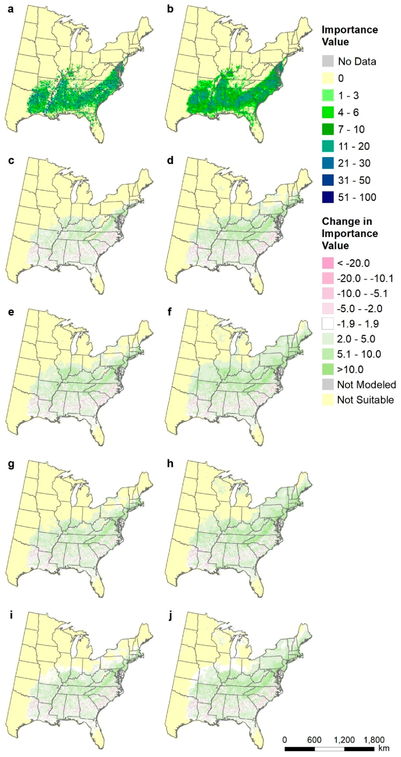
Figure A1.
Species distributions for Pinus echinata (shortleaf pine), shown as differences from current modeled distribution (map b): (a) FIA estimate of current distribution of abundance, (b) modeled current distribution, (c) CCSM45, (d) CCSM85, (e) GFDL45, (f) GFDL85, (g) Had45, (h) Had85, (i) mean of all three RCP4.5, and (j) mean of all three RCP8.5.

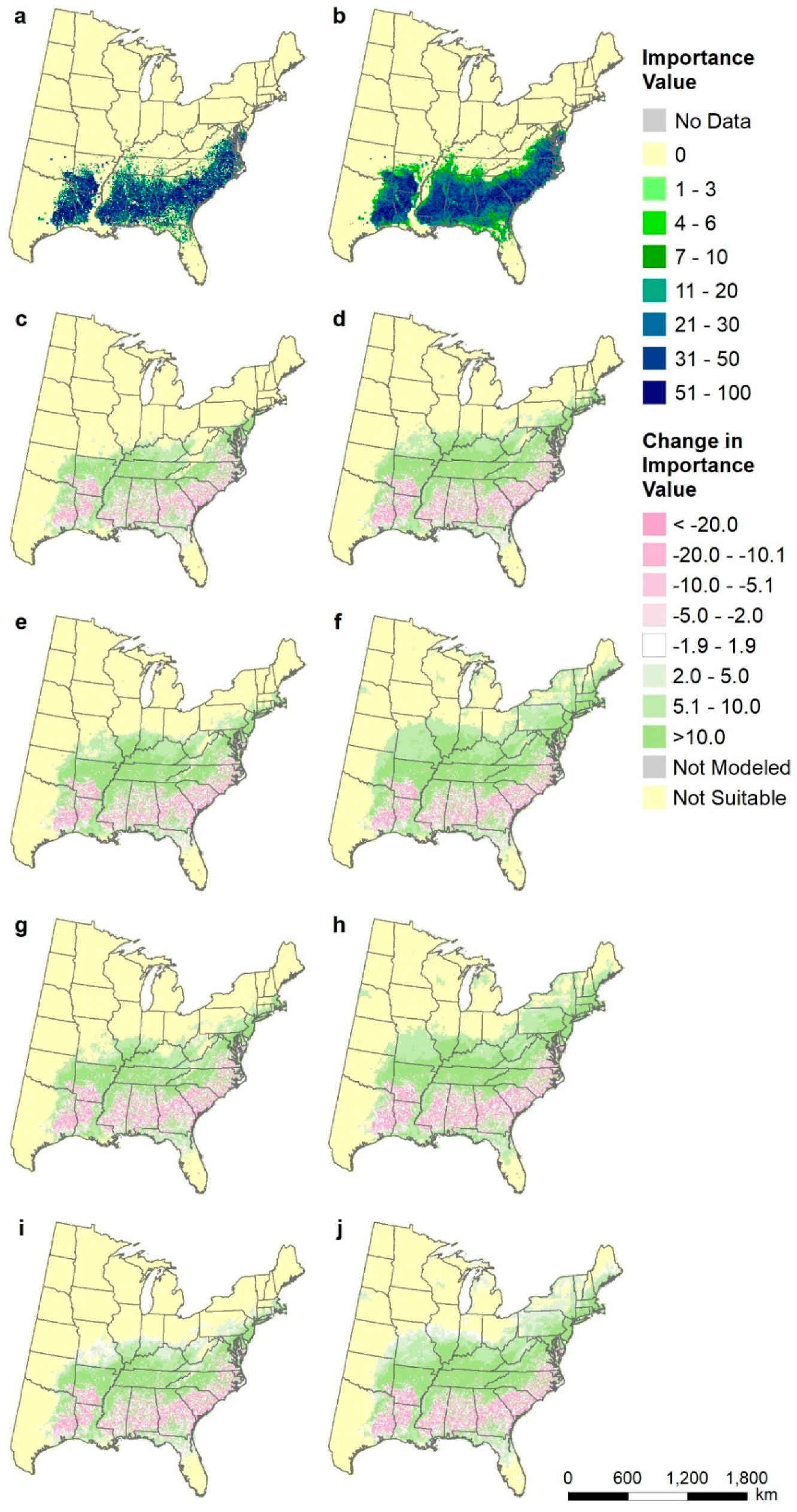
Figure A2.
Species distributions for Pinus teada (loblolly pine), shown as differences from current modeled distribution (map b): (a) FIA estimate of current distribution of abundance, (b) modeled current distribution, (c) CCSM45, (d) CCSM85, (e) GFDL45, (f) GFDL85, (g) Had45, (h) Had85, (i) mean of all three RCP4.5, and (j) mean of all three RCP8.5.

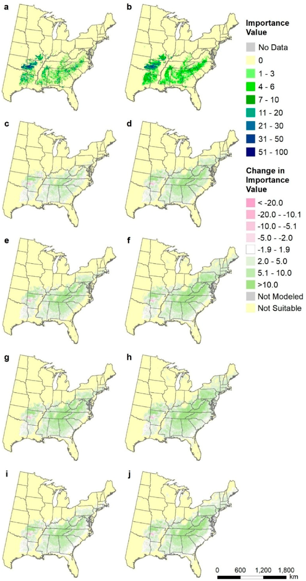
Figure A3.
Species distributions for Liquidambar styraciflua (sweetgum), shown as differences from current modeled distribution (map b): (a) FIA estimate of current distribution of abundance, (b) modeled current distribution, (c) CCSM45, (d) CCSM85, (e) GFDL45, (f) GFDL85, (g) Had45, (h) Had85, (i) mean of all three RCP4.5, and (j) mean of all three RCP8.5.

References
- Mora, C.; Spirandelli, D.; Franklin, E.C.; Lynham, J.; Kantar, M.B.; Miles, W.; Smith, C.Z.; Freel, K.; Moy, J.; Louis, L.V.; et al. Broad threat to humanity from cumulative climate hazards intensified by greenhouse gas emissions. Nat. Clim. Chang. 2018. [Google Scholar] [CrossRef]
- Hsiang, S.; Kopp, R.; Jina, A.; Rising, J.; Delgado, M.; Mohan, S.; Rasmussen, D.J.; Muir-Wood, R.; Wilson, P.; Oppenheimer, M.; et al. Estimating economic damage from climate change in the United States. Science 2017, 356, 1362–1369. [Google Scholar] [CrossRef] [PubMed] [Green Version]
- IPCC Summary for Policymakers. In Global Warming of 1.5 °C. An IPCC Special Report on the Impacts of Global Warming of 1.5 °C Above Pre-Industrial Levels and Related Global Greenhouse Gas Emission Pathways, in the Context of Strengthening the Global Response to the Threat of Climate Change, Sustainable Development, and Efforts to Eradicate Poverty; World Meteorological Organization: Geneva, Switzerland, 2018; p. 32.
- Rogelj, J.; den Elzen, M.; Höhne, N.; Fransen, T.; Fekete, H.; Winkler, H.; Schaeffer, R.; Sha, F.; Riahi, K.; Meinshausen, M. Paris Agreement climate proposals need a boost to keep warming well below 2 °C. Nature 2016, 534, 631. [Google Scholar] [CrossRef] [PubMed]
- Warren, R.; Price, J.; Graham, E.; Forstenhaeusler, N.; VanDerWal, J. The projected effect on insects, vertebrates, and plants of limiting global warming to 1.5 °C rather than 2 °C. Science 2018, 360, 791–795. [Google Scholar] [CrossRef]
- Swanston, C.W.; Janowiak, M.; Brandt, L.; Butler, P.; Handler, S.D.; Shannon, P.D.; Lewis, A.D.; Hall, K.R.; Fahey, R.T.; Scott, L.; et al. Forest Adaptation Resources: Climate Change Tools and Approaches for Land Managers, 2nd ed.; Gen. Tech. Rep. NRS-GTR-87-2; U.S. Department of Agriculture, Forest Service, Northern Research Station: Newtown Square, PA, USA, 2016; p. 161.
- Millar, C.; Stephenson, N.L. Climate change and forests of the future: Managing in the face of uncertainty. Ecol. Appl. 2007, 17, 2145–2151. [Google Scholar] [CrossRef] [PubMed]
- Nagel, L.M.; Palik, B.J.; Battaglia, M.A.; D’Amato, A.W.; Guldin, J.M.; Swanston, C.W.; Janowiak, M.K.; Powers, M.P.; Joyce, L.A.; Millar, C.I.; et al. Adaptive Silviculture for Climate Change: A National Experiment in Manager-Scientist Partnerships to Apply an Adaptation Framework. J. For. 2017, 115, 167–178. [Google Scholar] [CrossRef]
- Halofsky, J.E.; Andrews-Key, S.A.; Edwards, J.E.; Johnston, M.H.; Nelson, H.W.; Peterson, D.L.; Schmitt, K.M.; Swanston, C.W.; Williamson, T.B. Adapting forest management to climate change: The state of science and applications in Canada and the United States. For. Ecol. Manag. 2018, 421, 84–97. [Google Scholar] [CrossRef]
- Iverson, L.; McKenzie, D. Tree-species range shifts in a changing climate—Detecting, modeling, assisting. Landsc. Ecol. 2013, 28, 879–889. [Google Scholar] [CrossRef]
- Lenoir, J.; Svenning, J.C. Climate-related range shifts—A global multidimensional synthesis and new research directions. Ecography 2014, 38, 15–28. [Google Scholar] [CrossRef]
- Vanderwel, M.C.; Rozendaal, D.M.A.; Evans, M.E.K. Predicting the abundance of forest types across the eastern U.S. through inverse modelling of tree demography. Ecol. Appl. 2017, 27, 2128–2141. [Google Scholar] [CrossRef]
- Clark, J.S.; Nemergut, D.; Seyednasrollah, B.; Turner, P.J.; Zhang, S. Generalized joint attribute modeling for biodiversity analysis: Median-zero, multivariate, multifarious data. Ecol. Monogr. 2016, 87, 34–56. [Google Scholar] [CrossRef]
- DeHayes, D.H.; Jacobson, G.L.; Schaberg, P.G.; Bongarten, B.; Iverson, L.R.; Dieffenbacker-Krall, A. Forest responses to changing climate: Lessons from the past and uncertainty for the future. In Responses of Northern Forests to Environmental Change; Mickler, R.A., Birdsey, R.A., Hom, J.L., Eds.; Springer, Ecological Studies Series: New York, NY, USA, 2000; pp. 495–540. [Google Scholar]
- Delcourt, P.A.; Delcourt, H.R. Late-Quaternary dynamics of temperate forests—Applications of paleoecology to issues of global environmental-change. Quat. Sci. Rev. 1987, 6, 129–146. [Google Scholar] [CrossRef]
- Koo, K.A.; Madden, M.; Patten, B.C. Projection of red spruce (Picea rubens Sargent) habitat suitability and distribution in the Southern Appalachian Mountains, USA. Ecol. Model. 2014, 293, 91–101. [Google Scholar] [CrossRef]
- Prasad, A.M.; Iverson, L.R.; Matthews, S.N.; Peters, M.P. A multistage decision support framework to guide tree species management under climate change via habitat suitability and colonization models, and a knowledge-based scoring system. Landsc. Ecol. 2016, 31, 2187–2204. [Google Scholar] [CrossRef]
- Iverson, L.; Prasad, A.M.; Matthews, S.; Peters, M. Lessons learned while integrating habitat, dispersal, disturbance, and life-history traits into species habitat models under climate change. Ecosystems 2011, 14, 1005–1020. [Google Scholar] [CrossRef]
- Morin, X.; Thuiller, W. Comparing niche- and process-based models to reduce prediction uncertainty in species range shifts under climate change. Ecology 2009, 90, 1301–1313. [Google Scholar] [CrossRef] [PubMed]
- Iverson, L.R.; Thompson, F.R.; Matthews, S.; Peters, M.; Prasad, A.; Dijak, W.D.; Fraser, J.; Wang, W.J.; Hanberry, B.; He, H.; et al. Multi-model comparison on the effects of climate change on tree species in the eastern U.S.: Results from an enhanced niche model and process-based ecosystem and landscape models. Landsc. Ecol. 2017, 32, 1327–1346. [Google Scholar] [CrossRef]
- Johnstone, J.F.; Allen, C.D.; Franklin, J.F.; Frelich, L.E.; Harvey, B.J.; Higuera, P.E.; Mack, M.C.; Meentemeyer, R.K.; Metz, M.R.; Perry, G.L.; et al. Changing disturbance regimes, ecological memory, and forest resilience. Front. Ecol. Environ. 2016, 14, 369–378. [Google Scholar] [CrossRef]
- Kullman, L. Rapid recent range-margin rise of tree and shrub species in the Swedish Scandes. J. Ecol. 2002, 90, 68–77. [Google Scholar] [CrossRef] [Green Version]
- Gamache, I.; Payette, S. Latitudinal response of subarctic tree lines to recent climate change in eastern Canada. J. Biogeogr. 2005, 32, 849–862. [Google Scholar] [CrossRef]
- Holzinger, B.; Hulber, K.; Camenisch, M.; Grabherr, G. Changes in plant species richness over the last century in the eastern Swiss Alps: Elevational gradient, bedrock effects and migration rates. Plant Ecol. 2008, 195, 179–196. [Google Scholar] [CrossRef]
- Lenoir, J.; Gégout, J.C.; Marquet, P.A.; de Ruffray, P.; Brisse, H. A significant upward shift in plant species optimum elevation during the 20th century. Science 2008, 320, 1768–1771. [Google Scholar] [CrossRef]
- Hillyer, R.; Silman, M.R. Changes in species interactions across a 2.5 km elevation gradient: Effects on plant migration in response to climate change. Glob. Chang. Biol. 2010, 16, 3205–3214. [Google Scholar] [CrossRef]
- Felde, V.A.; Kapfer, J.; Grytnes, J.-A. Upward shift in elevational plant species ranges in Sikkilsdalen, central Norway. Ecography 2012, 35, 922–932. [Google Scholar] [CrossRef] [Green Version]
- Freeman, B.G.; Lee-Yaw, J.A.; Sunday, J.M.; Hargreaves, A.L. Expanding, shifting and shrinking: The impact of global warming on species’ elevational distributions. Glob. Ecol. Biogeogr. 2018, 27, 1268–1276. [Google Scholar] [CrossRef]
- Foster, J.R.; D’Amato, A.W. Montane forest ecotones moved downslope in northeastern US in spite of warming between 1984 and 2011. Glob. Chang. Biol. 2015, 21, 4497–4507. [Google Scholar] [CrossRef] [PubMed]
- Beckage, B.; Osborne, B.; Gavin, D.G.; Pucko, C.; Siccama, T.; Perkins, T. A rapid upward shift of a forest ecotone during 40 years of warming in the Green Mountains of Vermont. Proc. Natl. Acad. Sci. USA 2008, 105, 4197–4202. [Google Scholar] [CrossRef] [Green Version]
- Morin, R.S.; Liebhold, A.M. Invasive forest defoliator contributes to the impending downward trend of oak dominance in eastern North America. For. Int. J. For. Res. 2015, 89, 284–289. [Google Scholar] [CrossRef] [Green Version]
- Dolan, B.K.J. Forest regeneration following emerald ash borer (Agrilus planipennis Fairemaire) enhances mesophication in eastern hardwood forests. Forests 2018, 9, 353. [Google Scholar] [CrossRef]
- Wang, W.; He, H.; Thompson, F., III; Fraser, J.; Hanberry, B.; Dijak, W. The importance of succession, harvest, and climate change in determining future forest composition changes in U.S. Central Hardwood Forests. Ecosphere 2015, 6, art277. [Google Scholar] [CrossRef]
- Hanberry, B.B.; Hansen, M.H. Latitudinal range shifts of tree species in the United States across multi-decadal time scales. Basic Appl. Ecol. 2015, 16, 231–238. [Google Scholar] [CrossRef]
- Boisvert-Marsh, L.; Périé, C.; de Blois, S. Shifting with climate? Evidence for recent changes in tree species distribution at high latitudes. Ecosphere 2014, 5, 1–33. [Google Scholar] [CrossRef]
- Boisvert-Marsh, L.; Périé, C.; de Blois, S. Divergent responses to climate change and disturbance drive recruitment patterns underlying latitudinal shifts of tree species. J. Ecol. 2019. [Google Scholar] [CrossRef]
- Sittaro, F.; Paquette, A.; Messier, C.; Nock Charles, A. Tree range expansion in eastern North America fails to keep pace with climate warming at northern range limits. Glob. Chang. Biol. 2017, 23, 3292–3301. [Google Scholar] [CrossRef]
- Woodall, C.W.; Westfall, J.A.; D’Amato, A.W.; Foster, J.R.; Walters, B.F. Decadal changes in tree range stability across forests of the eastern U.S. For. Ecol. Manag. 2018, 429, 503–510. [Google Scholar] [CrossRef]
- Iverson, L.R.; Prasad, A.M. Predicting abundance of 80 tree species following climate change in the eastern United States. Ecol. Monogr. 1998, 68, 465–485. [Google Scholar] [CrossRef]
- Iverson, L.R.; Prasad, A.M.; Hale, B.J.; Sutherland, E.K. Atlas of Current and Potential Future Distributions of Common Trees of the Eastern United States; General Technical Report NE-265; Northeastern Research Station, USDA Forest Service: Radnor, PA, USA, 1999; p. 245.
- Prasad, A.M.; Iverson, L.R.; Liaw, A. Newer classification and regression tree techniques: Bagging and random forests for ecological prediction. Ecosystems 2006, 9, 181–199. [Google Scholar] [CrossRef]
- Iverson, L.R.; Prasad, A.M.; Matthews, S.N.; Peters, M. Estimating potential habitat for 134 eastern US tree species under six climate scenarios. For. Ecol. Manag. 2008, 254, 390–406. [Google Scholar] [CrossRef]
- Iverson, L.R.; Prasad, A.M.; Matthews, S.N. Modeling potential climate change impacts on the trees of the northeastern United States. Mitig. Adapt. Strateg. Glob. Chang. 2008, 13, 487–516. [Google Scholar] [CrossRef]
- Butler-Leopold, P.R.; Iverson, L.R.; Thompson, F.R., III; Brandt, L.A.; Handler, S.D.; Janowiak, M.K.; Shannon, P.D.; Swanston, C.W.; Bearer, S.; Bryan, A.M.; et al. Mid-Atlantic Forest Ecosystem Vulnerability Assessment and Synthesis: A Report from the Mid-Atlantic Climate Change Response Framework Project; Gen. Tech. Rep. NRS-181; U.S. Department of Agriculture, Forest Service, Northern Research Station: Newtown Square, PA, USA, 2018; p. 365.
- Butler, P.R.; Iverson, L.; Thompson, F.R.; Brandt, L.; Handler, S.; Janowiak, M.; Shannon, P.D.; Swanston, C.; Karriker, K.; Bartig, J.; et al. Central Appalachians Forest Ecosystem Vulnerability Assessment and Synthesis: A Report from the Central Appalachians Climate Change Response Framework Project; U.S. Department of Agriculture, Forest Service, Northern Research Station: Newtown Square, PA, USA, 2015; p. 310.
- Brandt, L.; He, H.; Iverson, L.; Thompson, F.; Butler, P.; Handler, S.; Janowiak, M.; Swanston, C.; Albrecht, M.; Blume-Weaver, R.; et al. Central Hardwoods Ecosystem Vulnerability Assessment and Synthesis: A Report from the Central Hardwoods Climate Change Response Framework Project; U.S. Department of Agriculture, Forest Service, Northern Research Station: Newtown Square, PA, USA, 2014; p. 254.
- Handler, S.; Duveneck, M.; Iverson, L.; Peters, E.; Scheller, R.; Wythers, K.; Brandt, L.; Butler, P.; Janowiak, M.; Swanston, C.; et al. Minnesota Forest Ecosystem Vulnerability Assessment and Synthesis: A report from the Northwoods Climate Change Response Framework; Gen. Tech. Rep. NRS-133; U.S. Department of Agriculture, Forest Service, Northern Research Station: Newtown Square, PA, USA, 2014.
- Handler, S.; Duveneck, M.J.; Iverson, L.; Peters, E.; Scheller, R.; Wythers, K.; Brandt, L.; Butler, P.; Janowiak, M.; Swanston, C.; et al. Michigan Forest Ecosystem Vulnerability Assessment and Synthesis: A Report from the Northwoods Climate Change Response Framework; Gen. Tech. Rep. NRS-129; U.S. Department of Agriculture, Forest Service, Northern Research Station: Newtown Square, PA, USA, 2014.
- Janowiak, M.K.; Iverson, L.R.; Mladenoff, D.J.; Peters, E.; Wythers, K.R.; Xi, W.; Brandt, L.A.; Butler, P.R.; Handler, S.D.; Shannon, P.D.; et al. Forest Ecosystem Vulnerability Assessment and Synthesis for Northern Wisconsin and Western Upper Michigan: A Report from the Northwoods Climate Change Response Framework Project; Gen. Tech. Rep. NRS-136; U.S. Department of Agriculture, Forest Service, Northern Research Station: Newtown Square, PA, USA, 2014; p. 247.
- Janowiak, M.K.; D’Amato, A.W.; Swanston, C.W.; Iverson, L.; Thompson, F., III; Dijak, W.; Matthews, S.; Peters, M.; Prasad, A.; Fraser, J.; et al. New England and Northern New York Forest Ecosystem Vulnerability Assessment and Synthesis: A Report from the New England Climate Change Response Framework Project; Gen. Tech. Rep. NRS-173; U.S. Department of Agriculture, Forest Service, Northern Research Station: Newtown Square, PA, USA, 2018; p. 234.
- Brandt, L.A.; Derby Lewis, A.; Scott, L.; Darling, L.; Fahey, R.T.; Iverson, L.; Nowak, D.J.; Bodine, A.R.; Bell, A.; Still, S.; et al. Chicago Wilderness Region Urban Forest Vulnerability Assessment and Synthesis: A Report from the Urban Forestry Climate Change Response Framework Chicago Wilderness Pilot Project; U.S. Department of Agriculture, Forest Service, Northern Research Station: Newtown Square, PA, USA, 2017; p. 142.
- Soil_Survey_Staff. Gridded Soil Survey Geographic (gSSURGO) Database for Ohio; United States Department of Agriculture, Natural Resources Conservation Service. Available online: https://gdg.sc.egov.usda.gov/ (accessed on 24 May 2016).
- Daly, C.; Halbleib, M.; Smith, J.I.; Gibson, W.P.; Doggett, M.K.; Taylor, G.H.; Curtis, J.; Pasteris, P.P. Physiographically sensitive mapping of climatological temperature and precipitation across the conterminous United States. Int. J. Climatol. 2008, 28, 2031–2064. [Google Scholar] [CrossRef] [Green Version]
- Thrasher, B. Downscaled Climate Projections Suitable for Resource Management. Eos 2013, 94, 321–323. [Google Scholar] [CrossRef]
- Maurer, E.P.; Hidalgo, H.G. Utility of daily vs. monthly large-scale climate data: An intercomparison of two statistical downscaling methods. Hydrol. Earth Syst. Sci. 2008, 12, 551–563. [Google Scholar] [CrossRef]
- Monahan, W.B.; Cook, T.; Melton, F.; Connor, J.; Bobowski, B. Forecasting Distributional Responses of Limber Pine to Climate Change at Management-Relevant Scales in Rocky Mountain National Park. PLoS ONE 2013, 8, e83163. [Google Scholar] [CrossRef]
- Moss, R.; Babiker, W.; Brinkman, S.; Calvo, E.; Carter, T.; Edmonds, J.; Elgizouli, I.; Emori, S.; Erda, L.; Hibbard, K. Towards New Scenarios for the Analysis of Emissions, Climate Change, Impacts, and Response Strategies; Intergovernmental Panel on Climate Change: Geneva, Switzerland, 2008; p. 25. ISBN 978-92-9169-124-1. [Google Scholar]
- Gent, P.R.; Danabasoglu, G.; Donner, L.J.; Holland, M.M.; Hunke, E.C.; Jayne, S.R.; Lawrence, D.M.; Neale, R.B.; Rasch, P.J.; Vertenstein, M.; et al. The Community Climate System Model Version 4. J. Clim. 2011, 24, 4973–4991. [Google Scholar] [CrossRef] [Green Version]
- Donner, L.J.; Wyman, B.L.; Hemler, R.S.; Horowitz, L.W.; Ming, Y.; Zhao, M.; Golaz, J.-C.; Ginoux, P.; Lin, S.J.; Schwarzkopf, M.D.; et al. The Dynamical Core, Physical Parameterizations, and Basic Simulation Characteristics of the Atmospheric Component AM3 of the GFDL Global Coupled Model CM3. J. Clim. 2011, 24, 3484–3519. [Google Scholar] [CrossRef]
- Collins, W.J.; Bellouin, N.; Doutriaux-Boucher, M.; Gedney, N.; Halloran, P.; Hinton, T.; Hughes, J.; Jones, C.D.; Joshi, M.; Liddicoat, S.; et al. Development and evaluation of an Earth-System model—HadGEM2. Geosci. Model Dev. 2011, 4, 1051–1075. [Google Scholar] [CrossRef]
- Jones, C.D.; Hughes, J.K.; Bellouin, N.; Hardiman, S.C.; Jones, G.S.; Knight, J.; Liddicoat, S.; O’Connor, F.M.; Andres, R.J.; Bell, C.; et al. The HadGEM2-ES implementation of CMIP5 centennial simulations. Geosci. Model Dev. 2011, 4, 543–570. [Google Scholar] [CrossRef] [Green Version]
- Peters, M.P.; Iverson, L. Projected Drought for the Conterminous United States in the 21st Century. In Drought Impacts on U.S. Forests and Rangelands: Translating Science into Management Responses; Vose, J.M., Peterson, D.L., Luce, C.H., Patel-Weynand, T., Eds.; Gen. Tech. Rep. WO-GTR-xx; U.S. Department of Agriculture, Forest Service: Washington, DC, USA, in press.
- Farr, T.G.; Rosen, P.A.; Caro, E.; Crippen, R.; Duren, R.; Hensley, S.; Kobrick, M.; Paller, M.; Rodriguez, E.; Roth, L.; et al. The Shuttle Radar Topography Mission. Rev. Geophys. 2007, 45. [Google Scholar] [CrossRef]
- Forsythe, W.C.; Rykiel, E.J.; Stahl, R.S.; Wu, H.-I.; Schoolfield, R.M. A model comparison for daylength as a function of latitude and day of year. Ecol. Model. 1995, 80, 87–95. [Google Scholar] [CrossRef]
- Schaetzl, R.J.; Krist, F.J.J.; Miller, B.A. A taxonomically based ordinal estimate of soil productivity for landscape-scale analyses. Soil Sci. Soc. Am. J. 2012, 75, 1–8. [Google Scholar] [CrossRef]
- Koch, F.H.; Smith, W.D.; Coulston, J.W. An Improved Method for Standardized Mapping of Drought Conditions. In Forest Health Monitoring: National Status, Trends, and Analysis 2010; Gen. Tech. Rep. SRS-GTR-176; Potter, K.M., Conkling, B.L., Eds.; U.S. Department of Agriculture Forest Service, Southern Research Station: Asheville, NC, USA, 2013; p. 164. [Google Scholar]
- Liaw, A.; Wiener, M. Classification and regression by randomForest. R News 2002, 2, 18–22. [Google Scholar]
- R_Development_Core_Team. R: A Language and Environment for Statistical Computing. Version 3.1.1; R Foundation for Statistical Computing: Vienna, Austria, 2014. [Google Scholar]
- Fry, J.A.; Xian, G.; Jin, S.; Dewitz, J.A.; Homer, C.G.; LIMIN, Y.; Barnes, C.A.; Herold, N.D.; Wickham, J.D. Completion of the 2006 national land cover database for the conterminous United States. Photogramm. Eng. Remote Sens. 2011, 77, 858–864. [Google Scholar]
- Breiman, L. Random forests. Mach. Learn. 2001, 45, 5–32. [Google Scholar] [CrossRef]
- Roy, M.-H.; Larocque, D. Robustness of random forests for regression. J. Nonparametric Stat. 2012, 24, 993–1006. [Google Scholar] [CrossRef]
- Hagen-Zanker, A. Comparing Continuous Valued Raster Data: A Cross Disciplinary Literature Scan; Research Institute for Knowledge Systems: Bilthoven, The Netherlands, 2006. [Google Scholar]
- Iverson, L.R.; Schwartz, M.W.; Prasad, A. How fast and far might tree species migrate under climate change in the eastern United States? Glob. Ecol. Biogeogr. 2004, 13, 209–219. [Google Scholar] [CrossRef]
- Iverson, L.R.; Schwartz, M.W.; Prasad, A.M. Potential colonization of new available tree species habitat under climate change: An analysis for five eastern US species. Landsc. Ecol. 2004, 19, 787–799. [Google Scholar] [CrossRef]
- Prasad, A.M.; Gardiner, J.; Iverson, L.; Matthews, S.; Peters, M. Exploring tree species colonization potentials using a spatially explicit simulation model: Implications for four oaks under climate change. Glob. Chang. Biol. 2013, 19, 2196–2208. [Google Scholar] [CrossRef]
- Clark, J.; Iverson, L.; Woodall, C.W.; Allen, C.D.; Bell, D.M.; Bragg, D.C.; D’Amato, A.W.; Davis, F.W.; Hersh, M.H.; Ibanez, I.; et al. Impacts of increasing drought on forest dynamics, structure, diversity, and management. In Effects of Drought on Forests and Rangelands in the United States: A Comprehensive Science Synthesis; Vose, J., Clark, J., Luce, C., Patel-Weynand, T., Eds.; Gen. Tech. Rep. WO-93b; U.S. Department of Agriculture, Forest Service, Washington Office: Washington, DC, USA, 2016; pp. 59–96. [Google Scholar]
- Dukes, J.S.; Pontius, J.; Orwig, D.; Garnas, J.R.; Rodgers, V.L.; Brazee, N.; Cooke, B.; Theoharides, K.A.; Stange, E.E.; Harrington, R.; et al. Responses of insect pests, pathogens, and invasive plant species to climate change in the forests of northeastern North America: What can we predict? Can. J. For. Res. 2009, 39, 231–248. [Google Scholar] [CrossRef]
- Fei, S.; Desprez, J.M.; Potter, K.M.; Jo, I.; Knott, J.A.; Oswalt, C.M. Divergence of species responses to climate change. Sci. Adv. 2017, 3, e1603055. [Google Scholar] [CrossRef] [PubMed] [Green Version]
- Matthews, S.N.; Iverson, L.; Peters, M.; Prasad, A.M. Assessing Potential Climate Change Pressures Throughout This Century across the Conterminous United States: Mapping Plant Hardiness Zones, Heat Zones, Growing Degree Days, and Cumulative Drought Severity Throughout this Century Research Map NRS-9; U.S. Department of Agriculture, Forest Service. Northern Research Station: Newtown Square, PA, USA, 2018; p. 31.
- Iverson, L.; Matthews, S.; Prasad, A.; Peters, M.; Yohe, G. Development of risk matrices for evaluating climatic change responses of forested habitats. Clim. Chang. 2012, 114, 231–243. [Google Scholar] [CrossRef] [Green Version]
- Matthews, S.N.; Iverson, L.R.; Prasad, A.M.; Peters, M.P.; Rodewald, P.G. Modifying climate change habitat models using tree species-specific assessments of model uncertainty and life history-factors. For. Ecol. Manag. 2011, 262, 1460–1472. [Google Scholar] [CrossRef]
- Box, G.; Draper, N.R. Empirical Model-Building and Response Surfaces; Wiley: New York, NY, USA, 1987. [Google Scholar]
Figure 1.
Distribution of annual temperature and precipitation changes from a baseline period (1981–2010) as modeled by the NASA Earth Exchange U.S. Downscaled Climate Projections (NEX-US-DCP30) data for 2070–2099, for 41,683 10-km cells across the eastern US. Black dots are the mean change in precipitation and temperature for each General Circulation Models (GCM)- Representative Concentration Pathways (RCP) scenario.

Figure 2.
Extent of 20 km vs. 10 km cells used for DISTRIB-II modeling.

Figure 3.
Potential changes in distance and direction of mean centers of suitable habitat for each of 125 species, according to (a) CCSM45, (b) GCM45, (c) GCM85), and (d) GFDL85. These are the ‘bookends’ of severity (CCSM45 and Had85) and the means (GCM45 and GCM85) of all three models.
Figure 3.
Potential changes in distance and direction of mean centers of suitable habitat for each of 125 species, according to (a) CCSM45, (b) GCM45, (c) GCM85), and (d) GFDL85. These are the ‘bookends’ of severity (CCSM45 and Had85) and the means (GCM45 and GCM85) of all three models.

Figure 4.
Ellipses of 1 standard deviation and mean centers for the current distribution and suitable habitat according to CCSM45, GCM45, GCM85, and Had85 under RCP 4.5 (circles) and 8.5 (squares) for (A) Liquidambar styraciflua and (B) Pinus echinata. Only the ‘bookends’ of severity (CCSM45 and Had85) and the means (GCM45 and GCM85) of all three models are presented. FIA Actual refers to the known FIA plot locations of the species, while Current refers to the modeled current distribution of the species.

Figure 5.
Liriodendron tulipifera (yellow poplar) distributions, shown as differences from current modeled distribution (map b): (a) FIA estimate of current distribution of abundance, (b) modeled current distribution, (c) CCSM45, (d) CCSM85, (e) GFDL45, (f) GFDL85, (g) Had45, (h) Had85, (i) mean of all three RCP4.5, and (j) mean of all three RCP8.5.

Table 1.
Average climate conditions in the eastern US currently and for three models (CCSM4, GFDL CM3, and HadGEM2-ES) for the 4.5 and 8.5 RCPs. CCSM4: Community Climate System Model; GFDL CM3: Geophysical Fluid Dynamics Laboratory Coupled Model 3; HadGEM2-ES: Hadley Global Environment Model—Earth System; PANN: Mean Annual Precipitation; Pgrow: Precipitation in growing season; TANN: Mean Annual Temperature; Tgrow: Temperature during growing season (May–Sept); TSUMavg: Mean Temperature of Warmest Month; TWINavg: Mean Temperature in Coldest Month; TMin: Absolute Minimum Temperature; TMax: Absolute Maximum Temperature; RCP: Representative Concentration Pathway.
| Variable | CCSM4 | GFDL CM3 | HadGEM2-ES | ||||
|---|---|---|---|---|---|---|---|
| Current | RCP 4.5 | RCP 8.5 | RCP 4.5 | RCP 8.5 | RCP 4.5 | RCP 8.5 | |
| PANN (mm) | 1048 | 1113 | 1162 | 1203 | 1233 | 1121 | 1110 |
| Pgrow (mm) | 509 | 527 | 519 | 573 | 585 | 504 | 457 |
| TANN (°C) | 12.7 | 15.2 | 17.1 | 16.3 | 18.6 | 16.8 | 19.2 |
| Tgrow (°C) | 21.6 | 24.0 | 26.3 | 26.0 | 28.4 | 25.7 | 28.4 |
| TSUMavg (°C) | 24.8 | 26.6 | 28.1 | 28.1 | 29.7 | 28.0 | 29.9 |
| TWINavg (°C) | −0.9 | 1.2 | 2.1 | 1.6 | 2.0 | 1.3 | 3.3 |
| TMin (°C) | −11.3 | −8.6 | −6.5 | −7.2 | −5.7 | −7.4 | −4.0 |
| TMax (°C) | 33.8 | 35.9 | 39.3 | 39.1 | 42.5 | 38.5 | 41.9 |
Table 2.
Environmental data used to predict habitat suitability of eastern U.S. tree species. Data was either aggregated to 10 and 20 km grids or derived from aggregated data.
Table 2.
Environmental data used to predict habitat suitability of eastern U.S. tree species. Data was either aggregated to 10 and 20 km grids or derived from aggregated data.
| Category | Variable | Description | Native Resolution |
|---|---|---|---|
| Climate 1 | Annual precipitation | Mean 30-year (1981–2010) monthly precipitation (mm). | 800 m |
| May–Sept. precipitation | Mean 30-year (1981–2010) monthly precipitation for May–September (mm). | ||
| Annual mean temperature | Mean 30-year (1981–2010) monthly temperature (°C). | ||
| May–Sept. mean temperature | Mean 30-year (1981–2010) monthly temperature for May–September (°C). | ||
| Mean temperature of coldest month | Mean 30-year (1981–2010) monthly temperature of coldest month (°C). | ||
| Mean temperature of warmest month | Mean 30-year (1981–2010) monthly temperature of warmest month (°C). | ||
| Aridity Index | A conditional ratio of precipitation and Thornthwaite potential evapotranspiration (see [66]) | 10 and 20 km | |
| Elevation [63] | Minimum | Minimum value | 90 m |
| Mean | Mean value | ||
| Maximum | Maximum value | ||
| Median | Median value | ||
| Range | Range between minimum and maximum values | ||
| Standard deviation | Amount of deviance among elevation | ||
| Coefficient of variation | The CV of elevation | ||
| Solar [64] | Day length coefficient of variation | The CV of 12 monthly day lengths derived from the latitude of grid cells. | 10 and 20 km |
| Soil [52] | Available water capacity (cm) | The quantity of water that the soil is capable of storing for use by plants | 30 m |
| Available water supply (cm) | The total volume of water that should be available to plants when the soil, inclusive of rock fragments, is at field capacity | ||
| Bulk density (g/cm3) | The ovendry weight of the soil material <2 mm in size per unit volume of soil at water tension of 1/3 bar | ||
| Calcium carbonate | The percent of carbonates, by weight, in the fraction of the soil <2 mm in size | ||
| Cation-exchange capacity | The total amount of extractable cations that can be held by the soil, expressed in terms of milliequivalents per 100 grams of soil at neutrality (pH 7.0) or at some other stated pH | ||
| Depth to water table (cm) | Depth to a saturated zone in the soil | ||
| Permeability (cm/h) | Saturated hydraulic conductivity or the ease with which pores in a saturated soil transmit water | ||
| Erosion K factor | The susceptibility of a soil to sheet and rill erosion by water estimated by the percentage of silt, sand, and organic matter and on soil structure and saturated hydraulic conductivity | ||
| Erosion T factor (tons/acre/year) | An estimate of the maximum average annual rate of soil erosion by wind and/or water that can occur without affecting crop productivity over a sustained period | ||
| Percent clay | Mineral soil particles that are <0.002 mm in diameter | ||
| Percent sand | Mineral soil particles that are 0.05 mm to 2 mm in diameter | ||
| Percent silt | Mineral soil particles that are 0.002 to 0.05 mm in diameter | ||
| Organic matter content (% by weight) | Plant and animal residue in soil material <2 mm in diameter at various stages of decomposition | ||
| pH | A measure of acidity or alkalinity | ||
| Percent passing sieve No. 10 | Soil fraction passing a number 10 sieve (2.00 mm square opening) | ||
| Percent passing sieve No. 200 | Soil fraction passing a number 200 sieve (0.074 mm square opening) | ||
| Soil productivity [65] | Productivity Index derived from family-level Soil Taxonomy information | ||
| Soil taxonomic order | The percentage of taxonomic order | ||
| Soil texture | The percentage of clayey, loamy, sandy, or other texture class defined by USDA standard terms |
1 PRISM Climate Group. 2014. Oregon State University, http://prism.oregonstate.edu.
Table 3.
Potential species changes in area-weighted importance value for habitat suitability for 125 species in the eastern United States. Allowing for a 10% buffer around the future:current ratio of 1.0 (i.e., no change), values below 0.9 indicates a loss, while values above 1.1 indicate a gain in suitable habitat. Scenarios refer to model (CCSM, GFDL, Had, and mean of all three GCM models) and emission level (RCP 4.5 and 8.5).
| Future: Current Ratios of Importance Values | ||||||
|---|---|---|---|---|---|---|
| Scenario | <0.5 | 0.5–0.9 | 0.9–1.1 | 1.1–2 | >2 | Total |
| CCSM45 | 6 | 18 | 14 | 64 | 23 | 125 |
| CCSM85 | 7 | 16 | 13 | 40 | 49 | 125 |
| GFDL45 | 8 | 15 | 13 | 39 | 50 | 125 |
| GFDL85 | 6 | 18 | 10 | 31 | 60 | 125 |
| HAD45 | 7 | 20 | 12 | 38 | 48 | 125 |
| HAD85 | 8 | 24 | 8 | 35 | 50 | 125 |
| GCM45 | 8 | 17 | 11 | 47 | 42 | 125 |
| GCM85 | 7 | 19 | 9 | 35 | 55 | 125 |
Table 4.
Number of species by distance and generalized northward and southward direction of mean centers of suitable habitat for the 125 species in the eastern United States. Only the ‘bookends’ of severity (CCSM45 and Had85) and the means (GCM45 and GCM85) of all three models are presented.
Table 4.
Number of species by distance and generalized northward and southward direction of mean centers of suitable habitat for the 125 species in the eastern United States. Only the ‘bookends’ of severity (CCSM45 and Had85) and the means (GCM45 and GCM85) of all three models are presented.
| Scenario | Kilometers | |||||||
|---|---|---|---|---|---|---|---|---|
| <10 | 10–50 | 51–100 | 101–200 | 201–300 | 301–400 | >400 | Total | |
| Northward | ||||||||
| CCSM45 | 1 | 16 | 22 | 43 | 10 | 0 | 1 | 93 |
| GCM45 | 1 | 12 | 19 | 33 | 19 | 7 | 8 | 99 |
| GCM85 | 0 | 9 | 11 | 25 | 23 | 16 | 17 | 101 |
| Had85 | 0 | 8 | 17 | 22 | 19 | 18 | 16 | 100 |
| Southward | ||||||||
| CCSM45 | 0 | 7 | 7 | 10 | 1 | 5 | 2 | 32 |
| GCM45 | 0 | 0 | 5 | 9 | 2 | 5 | 5 | 26 |
| GCM85 | 0 | 3 | 2 | 6 | 4 | 3 | 6 | 24 |
| Had85 | 0 | 2 | 4 | 5 | 7 | 2 | 5 | 25 |
Table 5.
Top three species currently in each region and state, along with the future:current ratio of projected suitable habitat under low and high emission scenarios.
Table 5.
Top three species currently in each region and state, along with the future:current ratio of projected suitable habitat under low and high emission scenarios.
| State/Region | First Species | Low | High | Second Species | Low | High | Third Species | Low | High |
|---|---|---|---|---|---|---|---|---|---|
| Eastern U.S. | Pinus taeda | 1.21 | 1.32 | Acer rubrum | 0.99 | 0.92 | Liquidambar styraciflua | 1.48 | 1.73 |
| Northeast | Acer rubrum | 0.91 | 0.76 | Acer saccharum | 0.93 | 0.88 | Pinus strobus | 1.04 | 0.87 |
| North Central | Populus tremuloides | 0.71 | 0.61 | Acer rubrum | 1 | 0.93 | Acer saccharum | 1.03 | 0.98 |
| Great Plains | Ulmus americana | 1.44 | 1.74 | Celtis occidentalis | 1.53 | 1.58 | Juniperus virginiana | 2.64 | 3.07 |
| Southeast | Pinus taeda | 1.07 | 1.09 | Pinus elliottii | 1.31 | 1.42 | Liquidambar styraciflua | 1.34 | 1.43 |
| South Central | Pinus taeda | 1.2 | 1.2 | Liquidambar styraciflua | 1.35 | 1.42 | Quercus stellata | 2.15 | 2.44 |
| Alabama | Pinus taeda | 0.98 | 0.95 | Liquidambar styraciflua | 1.17 | 1.21 | Quercus nigra | 2.04 | 2.29 |
| Arkansas | Pinus taeda | 1.35 | 1.36 | Pinus echinata | 1.55 | 1.56 | Quercus alba | 0.84 | 0.82 |
| Connecticut | Acer rubrum | 0.7 | 0.54 | Betula lenta | 0.65 | 0.54 | Quercus rubra | 0.89 | 0.77 |
| District of Columbia | Liriodendron tulipifera | 0.34 | 0.29 | Fagus grandifolia | 0.44 | 0.44 | Quercus prinus | 0.5 | 0.49 |
| Delaware | Acer rubrum | 0.77 | 0.69 | Pinus taeda | 2.38 | 2.4 | Liquidambar styraciflua | 1 | 1.07 |
| Florida | Pinus elliottii | 0.93 | 0.89 | Pinus taeda | 1.31 | 1.46 | Quercus laurifolia | 1.17 | 1.15 |
| Georgia | Pinus taeda | 0.97 | 0.95 | Pinus elliottii | 1.19 | 1.27 | Liquidambar styraciflua | 1.23 | 1.29 |
| Iowa | Ulmus americana | 1.23 | 1.27 | Juglans nigra | 1.39 | 1.33 | Celtis occidentalis | 2.24 | 2.02 |
| Illinois | Ulmus americana | 1.29 | 1.47 | Quercus alba | 0.92 | 0.76 | Prunus serotina | 0.77 | 0.66 |
| Indiana | Acer saccharum | 0.73 | 0.64 | Prunus serotina | 0.74 | 0.6 | Fraxinus americana | 0.99 | 0.94 |
| Kansas | Ulmus americana | 1.15 | 1.23 | Celtis occidentalis | 1.07 | 1.06 | Maclura pomifera | 1.21 | 1.22 |
| Kentucky | Liriodendron tulipifera | 0.44 | 0.35 | Acer saccharum | 0.66 | 0.6 | Quercus alba | 1.01 | 0.95 |
| Louisiana | Pinus taeda | 0.97 | 0.92 | Liquidambar styraciflua | 1.13 | 1.14 | Quercus nigra | 2.2 | 2.32 |
| Massachusetts | Acer rubrum | 0.81 | 0.66 | Pinus strobus | 0.46 | 0.38 | Quercus rubra | 1.02 | 0.92 |
| Maryland | Acer rubrum | 0.8 | 0.72 | Pinus taeda | 2.32 | 2.67 | Liriodendron tulipifera | 0.65 | 0.47 |
| Maine | Abies balsamea | 0.53 | 0.5 | Acer rubrum | 1.35 | 1.24 | Picea rubens | 0.64 | 0.57 |
| Michigan | Acer rubrum | 0.98 | 0.87 | Acer saccharum | 0.82 | 0.74 | Populus tremuloides | 0.89 | 0.8 |
| Minnesota | Populus tremuloides | 0.66 | 0.56 | Picea mariana | 0.4 | 0.4 | Larix laricina | 1.21 | 1.17 |
| Missouri | Quercus alba | 0.57 | 0.52 | Quercus velutina | 0.95 | 0.86 | Quercus stellata | 1.74 | 1.94 |
| Mississippi | Pinus taeda | 1.09 | 1.01 | Liquidambar styraciflua | 1.19 | 1.2 | Quercus nigra | 2.05 | 2.27 |
| North Carolina | Pinus taeda | 1.21 | 1.24 | Acer rubrum | 0.79 | 0.77 | Liquidambar styraciflua | 1.28 | 1.39 |
| North Dakota | Quercus macrocarpa | 1.75 | 2.58 | Populus tremuloides | 0.42 | 0.33 | Acer negundo | 1.92 | 1.63 |
| Nebraska | Juniperus virginiana | 1.92 | 2.33 | Quercus macrocarpa | 1.59 | 1.57 | Ulmus americana | 2.1 | 2.51 |
| New Hampshire | Acer rubrum | 1.06 | 0.91 | Pinus strobus | 0.79 | 0.65 | Tsuga canadensis | 0.77 | 0.66 |
| New Jersey | Pinus rigida | 0.39 | 0.39 | Acer rubrum | 1.05 | 0.92 | Quercus alba | 1 | 0.83 |
| New York | Acer rubrum | 0.98 | 0.77 | Acer saccharum | 0.78 | 0.71 | Fagus grandifolia | 0.73 | 0.67 |
| Ohio | Acer rubrum | 0.47 | 0.4 | Acer saccharum | 0.89 | 0.79 | Prunus serotina | 0.67 | 0.55 |
| Oklahoma | Quercus stellata | 1.09 | 1.08 | Juniperus virginiana | 1.24 | 1.34 | Pinus echinata | 1.36 | 1.4 |
| Pennsylvania | Acer rubrum | 0.64 | 0.47 | Prunus serotina | 0.77 | 0.63 | Acer saccharum | 0.91 | 0.86 |
| Rhode Island | Acer rubrum | 0.62 | 0.52 | Pinus strobus | 0.55 | 0.42 | Quercus rubra | 0.72 | 0.62 |
| South Carolina | Pinus taeda | 0.86 | 0.81 | Liquidambar styraciflua | 1.08 | 1.09 | Quercus nigra | 1.8 | 2.03 |
| South Dakota | Quercus macrocarpa | 5.57 | 5.65 | Juniperus virginiana | 5.87 | 6.93 | Fraxinus pennsylvanica | 3.75 | 4.15 |
| Tennessee | Liriodendron tulipifera | 0.51 | 0.42 | Quercus alba | 1.13 | 1.08 | Acer rubrum | 0.81 | 0.83 |
| Texas | Pinus taeda | 0.97 | 0.9 | Juniperus ashei | 1.11 | 1.1 | Quercus virginiana | 1.49 | 1.55 |
| Virginia | Pinus taeda | 1.45 | 1.66 | Liriodendron tulipifera | 0.5 | 0.33 | Acer rubrum | 0.82 | 0.76 |
| Vermont | Acer saccharum | 0.61 | 0.57 | Acer rubrum | 1.39 | 1.25 | Fagus grandifolia | 0.76 | 0.72 |
| Wisconsin | Populus tremuloides | 0.7 | 0.62 | Acer rubrum | 0.97 | 0.8 | Acer saccharum | 0.94 | 0.92 |
| West Virginia | Acer rubrum | 0.71 | 0.61 | Liriodendron tulipifera | 0.84 | 0.56 | Acer saccharum | 0.84 | 0.73 |
© 2019 by the authors. Licensee MDPI, Basel, Switzerland. This article is an open access article distributed under the terms and conditions of the Creative Commons Attribution (CC BY) license (http://creativecommons.org/licenses/by/4.0/).
Share and Cite
MDPI and ACS Style
Iverson, L.R.; Peters, M.P.; Prasad, A.M.; Matthews, S.N. Analysis of Climate Change Impacts on Tree Species of the Eastern US: Results of DISTRIB-II Modeling. Forests 2019, 10, 302. https://doi.org/10.3390/f10040302
AMA Style
Iverson LR, Peters MP, Prasad AM, Matthews SN. Analysis of Climate Change Impacts on Tree Species of the Eastern US: Results of DISTRIB-II Modeling. Forests. 2019; 10(4):302. https://doi.org/10.3390/f10040302
Chicago/Turabian StyleIverson, Louis R., Matthew P. Peters, Anantha M. Prasad, and Stephen N. Matthews. 2019. "Analysis of Climate Change Impacts on Tree Species of the Eastern US: Results of DISTRIB-II Modeling" Forests 10, no. 4: 302. https://doi.org/10.3390/f10040302
Note that from the first issue of 2016, this journal uses article numbers instead of page numbers. See further details here.