Development of Nonlinear Parsimonious Forest Models Using Efficient Expansion of the Taylor Series: Applications to Site Productivity and Taper


1
Faculty of Mathematics and Computer Science, University of Bucharest, 010014 Bucharest, Romania
2
Bioinformatics Department, National Institute of Research and Development for Biological Sciences, 060031 Bucharest, Romania
3
Faculty of Administration and Business, University of Bucharest, 010014 Bucharest, Romania
4
College of Forestry, Oregon State University, Corvallis, OR 97331, USA
*
Author to whom correspondence should be addressed.
Forests 2020, 11(4), 458; https://doi.org/10.3390/f11040458
Submission received: 8 March 2020
/
Revised: 14 April 2020
/
Accepted: 15 April 2020
/
Published: 18 April 2020
(This article belongs to the Special Issue Modeling Forest Stand Dynamics, Growth and Yield)
Abstract
:The parameters of nonlinear forest models are commonly estimated with heuristic techniques, which can supply erroneous values. The use of heuristic algorithms is partially rooted in the avoidance of transformation of the dependent variable, which introduces bias when back-transformed to original units. Efforts were placed in computing the unbiased estimates for some of the power, trigonometric, and hyperbolic functions since only few transformations of the predicted variable have the corrections for bias estimated. The approach that supplies unbiased results when the dependent variable is transformed without heuristic algorithms, but based on a Taylor series expansion requires implementation details. Therefore, the objective of our study is to investigate the efficient expansion of the Taylor series that should be included in applications, such that numerical bias is not present. We found that five functions require more than five terms, whereas the arcsine, arccosine, and arctangent did not. Furthermore, the Taylor series expansion depends on the variance. We illustrated the results on two forest modeling problems, one at the stand level, namely site productivity, and one at individual tree level, namely taper. The models that are presented in the paper are unbiased, more parsimonious, and they have a RMSE comparable with existing less parsimonious models.
1. Introduction
Bayesian estimators and machine learning algorithms became popular for determining the parameters of nonlinear models, which, in many cases, are preferred over the traditional least square or maximum likelihood methods [1,2,3,4,5,6,7,8,9,10,11]. The diminishing presence in solving nonlinear problem of the method based on least square method is twofold. First, the least square method is sensitive to outliers [1]. Second, to obtain expected fit, in many instances the variables are transformed [2,3]. However, variable transformations did not necessarily supply the desired results even when the assumptions are met, particularly when the predicted values were changed [12,13,14]. The bias induced by the transformation of the dependent variable was noted early by Williams [15] and Cochran [16], but its formal removal was only developed for few transformations, the most popular being the one for the logarithm function of Finney [17]. The lack of bias correction did not stop researchers transforming the dependent variable without correcting it [18], even after the ground-breaking paper of Neyman and Scott [19], who proposed a framework for all functions investigated. The difficult implementation of the procedure that was advocated by Neyman and Scott [19] was overcome by Nelder and Wedderburn [20], who developed the generalized linear models (GLM). However, the assumptions of GLM restricted its application to few functions, the most popular being, arguably, the logistic function.
The arrival of the powerful microprocessors at the completion of the second millennium opened a new avenue of modeling complex nonlinear functions, namely heuristic techniques [21,22]. The start of the third millennium was marked by a surge of developments and implementations of heuristic based algorithms that are focused on the estimation of parameters, as in Pujol [23], Chen, et al. [24], or Yuan [25], to cite just a few. However, as sophisticated as the heuristic techniques are, they just provide an approximation of the exact solution. In many instances, the approximation is so close to some bounding solutions, which, from a practical perspective, there is no reason to spend additional efforts in attaining optimality [26]. However, there are instances, particularly in the process based modeling [27], when heuristic techniques supply wrong results. It is a simple exercise to find cases when common algorithms used for the estimation of nonlinear regression supply values for some parameters with opposite signs than the actual ones. A similar situation can be encountered when the parameters are estimated with the Bayesian approach [28]. We present a very simple example to reinforce the dependency of the parameters to be estimated on the procedure used for estimation. Let us assume that a process can be modeled with the following equation:
where x is the predictor, y the response variable, and .
The distribution of e in this case is F(0,), where F is the cumulative distribution function of e (proof in the Appendix A). Estimations of F and are not trivial, as they have a nonlinear shape (Appendix A). What is to be observed is that , which means that the arctangent transformation of a normally distributed variable does not bias the model.
If synthetic data are generated for x from 2 to 1000, then the parameters of Equation (1) are estimated while using the nonlinear model
The solution of Equation (2) depends on the nonlinear algorithm used in computations, as the SAS implementation of the Gauss-Newton algorithm supplies the values b0 =−0.0493, b1 = 0.0935, b2= 59.26, and b3 = 0.2575, whereas the steepest descent algorithm leads to b0 = 0.4131, b1 = −7.1168, b2 = 0.1912, and b3 = −4.1017. What is important to note is not the difference in values between the expected and the values used to generate the data, but the change in the sign, of only b2, which triggers a completely different interpretation of the model. According to the generating model, only b2 should be negative, whereas, for Gauss-Newton, b0 is negative and b2 is positive. A more dramatic situation is encountered when the steepest descent algorithm is used for estimation, as only b0 has the correct sign, the b1, b2, and b3 have the opposite signs. Therefore, caution should be exercised when heuristic algorithms are employed in the estimation of non-linear models, as the results could be incorrect, not because of the model, but because of the algorithm.
The limited number of functions available for formal estimation by the generalized linear models of Nelder and Wedderburn [20] or the complicated framework proposed by Neyman and Scott [19], Strimbu, et al. [29] estimated exactly the expected parameters of ten transformations that are commonly encountered in environmental modeling to address the lack of accuracy associated with heuristic techniques. Their findings allow for complex nonlinear models to be tested without concerns that the parameters depend on the algorithms used for the estimation. Lack of impact on the results of the algorithms and elimination of bias when the predicted variable is transformed advocate for combinations of nonlinear functions repeatedly, a feature that is inexistent in the current procedures.
In order to model nonlinear relationships, the predicted variable is transformed with a differentiable function f, such that a linear relationship between f(Y) and a set of predictor variables is obtained
where is the vector of coefficients for the predictor variables , and are the residuals, normally being distributed with mean 0 and variance , .
The transformation introduces bias when is back-transformed to , which must be corrected. The substance of the paper of Strimbu, Amarioarei, and Paun [29] lies in the computation of the unbiased estimates of the mean of that was obtained from Equation (3) for ten commonly used functions. For eight of these functions, the obtained estimates are using the Taylor expansion; therefore, they contain an infinite number of terms. To support their findings, simulated data were used to select the number of terms of the Taylor expansion series. However, real problems are often more complex than simulated data. Therefore, the objective of the present study is to present the applicability of the new framework by presenting two examples: one on site productivity and one on tree taper. An additional objective is to estimate an efficient Taylor series expansion that would provide unbiased results for the sine, cosine, tangent, arc sine, arc cosine, arc tangent, hyperbolic sine, and hyperbolic tangent functions (i.e., the eight transformations involving Taylor series expansion).
2. Methods
2.1. Foundation
Equation (3) allows for complex nonlinear transformations by compounding different functions. Knowing the unbiased estimate of the inverse of the function f advocates the successive incorporation of various functions until models that meet scientific rigor and fulfill the research assumptions are obtained. Based on Equation (3) , if only one transformation is executed, an unbiased estimation of given would be:
If a subsequent transformation, is needed, then an unbiased estimation of at would be [30]:
where is a normal distributed residual with mean 0 and variance .
In the eventuality that the succession of unbiased back-transformations contains a finite number of terms, the combinations of nonlinear functions do not include additional assumptions. However, if an infinite number of terms are formally needed, while only finite terms are used in computations, the compounding could lead to erroneous results. The truncation can have a significant impact on the estimation, even for models that only contain one transformation (Equation (4)). Therefore, the transformations that are considered in this study are only those from Strimbu, Amarioarei, and Paun [29] that contain a Taylor series expansion, meaning an infinite number of terms:
- Sine, , for which and
- Cosine, for which α = −(1 + ξ)/σ and β = (1 − ξ)/σ
- Tangent, . for which α = −ξ/σ and β = (1 − ξ)/σ
- Arcsine or inverse of sine, . for which α = −(π/2 + ξ)/σ and β = (π/2 − ξ)/σ
- Arccosine or inverse of cosine, , for which α = −ξ/σ and β = (π − ξ)/σ
- Arctangent or inverse of tangent, . for which Bn is the nth Bernoulli number that is computed with the recurrence formula and B0 = 1.
- hyperbolic sine, , for which α = −ξ/σ and β = (1 − ξ)/σ
- hyperbolic tangent, , for which α = −ξ/σ and β = (1 − ξ)/σ
where the symbols used in the Equations (6)–(13) are:
- n, k are natural numbers;
- is the combination of n taken k;
- and is the products of the even, or uneven, respectively, numbers less than, including, , or , respectively;
We will be using a factorial experiment to identify an efficient Taylor series expansion for Equations (6)–(13). The factors considered in the experiments will be the number of terms, which varies from 2 to 10, and the variance, which has four values. The number of terms was chosen to ensure that convergence to a desired accuracy is achieved, given that rarely polynomials of degree larger than five are having an impact on the Taylor series. The number of variances was selected to assess the influence of variability on the convergence of the Taylor series, given that Equations (6)–(13) depend not only on the predictor variables, but also on the variance. The values for which the number of terms would be computed were defined by the magnitude of the transformed variable, such that a large range of values can be attained (Table 1).
A multitude of recommendations exists to ensure accuracy for infinite series [21,22,31,32,33]. Among them, two different approaches are popular: one that is based on a preset value measuring the difference between two estimates obtained with consecutive number of terms [34], and one based on the scree plot method [35,36]. In this study, a preset value of the order of 10−5 is used, which, according to LeVeque [34], ensures a second order accuracy. The scree plot was adjusted from the multivariate analysis case [37] to the univariate case by looking at the rate of change that is associated with each terms. The number of terms to retain is determined while using method 3, as listed by Rencher [38] p. 398), namely, to drop the terms that form a curve relatively parallel to the abscissa. In our study, we considered that an efficiency Taylor series expansion is the series with the largest number of terms being supplied by the two approaches (i.e., preset value or scree plot).
2.2. Modeling Site Productivity for Norway Spruce (Picea abies L) in Carpathian Mountains
Norway spruce is the main economic species in the Carpathian Mountains and, consequently, a significant effort was carried in assessing its site productivity. Summary statistics of the field measurements were published in 1957 [39], but no models were developed at that time. In 2004, a polymorphic site productivity model with six parameters (Equation (17)) was published by Giurgiu and Draghiciu [40], which is currently enforced by the current Romanian regulations:
where
- height dominant is the height of dominant trees;
- t Lorey height is transformed Lorey’s height modeled with the expression ;
- SI is site index; and,
- a0, a1, a2, b0, b1, b2 are parameters determined by species.
Unfortunately, the Giurgiu and Draghiciu [40] models are biased, as it assumes that regressions are causal relationships, which was proven to be false [41]. Therefore, unbiased models need to be developed. Since the raw data are unavailable, we have generated the heights and age values from the summary statistics of Popescu-Zeletin [39]. Popescu-Zeletin [39] presented the change in height with age using five productivity classes. The classes were created by separating the measured height at each age in five equally spaced intervals. Even though the method of Popescu-Zeletin differs from the approach that is used by the Food and Agriculture Organization, which separates heights using quartiles [42]; the results are similar. For each age, we have randomly generated 50 heights that are uniformly distributed among the five productivity classes to mirror the original data. To avoid inclusion of extreme values, we have focused only on the class II, III, and IV, which have as site indices 31.8 m, 26.9 m, and 21. 9 m (base age 100 years).
Among the functions that are available for parsimonious nonlinear modeling, we have selected the hyperbolic tangent of the ratio between height and site index, SI (Equation (18)):
where SI is height at age 100 years.
Using the correlation coefficient as a guidance and following a series of trail and errors we found that can be used as predictor of f(height). Therefore, we computed the unbiased height with Equation (19).
where .
To assess the parsimonious model developed with Equations (18) and (19) in the context of the existing models, we compared it with the current models that were enforced by the Romanian forest administration [40], namely Equation (17). In many instances, nonlinear models are estimated with a Bayesian approach [2,4,43]. Therefore, we have used the Bayesian approach that was proposed by Stow, et al. [44] to correct the retransformation bias. We estimated the model with Stan [45], a probabilistic program for Bayesian inference, as implemented in R [46] through the rstan package [47]. The Bayesian estimates are supplied by a Markov chain Monte Carlo procedure, which depends on multiple parameters, among which the number of iterations is paramount. The Stan Development Team [47] recommends the use of four chains for Bayesian estimation, and Stow, Reckhow, and Qian [44] suggests a non-informative prior distribution, which we have used in our computations.
2.3. Taper Equations for Loblolly Pine (Pinus taeda L.) in East Louisiana
The second example of parametric parsimonious nonlinear models is focused on taper. Loblolly pine is the most important commercial tree species in the south eastern region of the USA and, consequently, was the subject of many taper models, McClure and Czaplewski [48], Cao, et al. [49], or Max and Burkhart [50], to list just few. However, most of the models have at least two parameters, except Lenhart, et al. [51], who has one parameter, sometimes one of them being adhoc identified (e.g., the point joining different sections of the stem). We have used the taper data of Fang and Strimbu to test the performances of the parametric parsimonious nonlinear models [52]. The dataset contains 18 trees with diameters measuring every meter plus the diameter at breast height. A set of four models was assessed on the data, and revealed that the bias ranges between −2.2 mm to −0.1 mm and the MAE is between 12.5 mm and 13.5 mm. By trial and error, we have found that the cosine transformation of the ratio between diameter, d, and double dbh (i.e., ) can be predicted from the sum of the product of log(total height) and the square root of relative height (i.e., height of diameter d/total height) with the ratio of the total height and square root of dbh:
where .
We computed the unbiased diameter along the stem with Equation (7).
Similarly to the height Equation (17), we have compared the parsimonious model of Equation (18) with an existing taper model. Among the models that were developed for loblolly pine, we have chosen the model 02 of Kozak [53], who was proven to be the most appropriate for the data used in the present study [4]. Furthermore, we compared the parametric estimates of Equation (18) and Kozak 02 with their Bayesian estimates, while using Stan [45], as implemented in R [46] through the rstan package [47]. The Bayesian estimates were based on four Markov chains, as recommended by [47] and a non-informative prior distribution, as suggested by Stow, Reckhow, and Qian [44].
2.4. Models Assessment
A mandatory requirement in the application of the parsimonious models represented by Equations (6)–(13) is that the residuals of the linear relationship between the transformed predicted variable and the predictors are normally distributed. Therefore, we have tested the normality assumption while using the Shapiro-Wilk test, as implemented in the base R [54].
We assessed the performance of each of the three models using four metrics: pseudo-R2, bias, mean absolute error, MAE, and root mean square error, RMSE, similarly to Stängle, et al. [55], Montealegre, et al. [56], and Bilskie and Hagen [57]:
where
- is the predicted value at age/diameter/time i,
- is the measured value at age/height/time i, and
- n is the number of observations.
3. Results
3.1. Foundation
The analysis of the eight transformations for which Taylor series expansion is presented revealed that, irrespective of the size of the variance, an efficient Taylor series has less than 10 terms (Figure 1, Figure 2, Figure 3, Figure 4, Figure 5, Figure 6, Figure 7 and Figure 8). The number of terms varies with the procedure used for selection, the scree plot constantly supplying less terms than the preset value. When the number of terms was chosen at the first encounter of a difference between the expectations computed with consecutive number of terms that is less than the preset value, and then the two selection procedures supplied similar results (i.e., at most one term apart), except for the hyperbolic tangent case, which was two terms apart. However, we have investigated the consistency of the convergence by requiring that the preset value be encountered at least two consecutive times. In this situation, the difference between the scree plot and the preset value procedures increased significantly (Table 1), sometimes with six terms (i.e., hyperbolic tangent). When considering that the objective of the study is to identify the number of terms that can be used in applications without introducing bias, even when induced by numerical rounding, we recommend to use in computation with more terms. Therefore, all subsequent discussions, except noted otherwise, refer to the results for which the preset value was encountered to at least two consecutive Taylor series estimates.
For all of the functions, the number of terms that are needed for convergence according to the scree plot was at most five, except for the hyperbolic tangent, for which six terms are needed (Table 1). The results support the selection of five terms implemented by Strimbu, Amarioarei, and Paun [29], except for the hyperbolic tangent function. Nevertheless, the accuracy of the estimation with five terms for the hyperbolic tangent case is of the order of 10−4. The addition of the consistent convergence constraint had a significant impact on the number of terms, regardless of the transformation. The difference between the results that were obtained when the preset value was passed once or twice increases with variance, from none (e.g., sine or cosine) to three times (i.e., tangent). Therefore, the usage of a reduced number of terms should be approached with caution, as it can lead to biased results.
The results that are based on simulations show that, without a significant loss of generality, the infinite sums can be approximated by a finite number of terms. Therefore, we rewrote the general form of each Taylor series expansion to only include the first N terms:
where is the predicted, back-transformed, variable
The term is given by
When considering that Ξn,k depends on the variance of the linear model and of the transformed prediction, once the number of significant terms is established the back-transformed variable is the product of the constant matrix C and the values defined by the linear regression. The C matrix is a triangular matrix that only depends on the number of terms and the transformation used, and not the data for which the model is developed. The matrix for 5, 10, and 20 terms is presented in the Supplementary Material S1. Therefore, the final nonlinear model can be written as a linear model.
3.2. Site Index Models for Norway Spruce
The site index model for the Romanian Norway spruce that was developed from Equation (17) is
Irrespective the site productivity class (i.e., II, III, or IV), the transformed model has a coefficient of determination > 0.9 (p-value < 0.001), showing the appropriateness of the models (Figure 9). The Shapiro-Wilk test suggests that residuals are likely to be normally distributed (p-value > 0.25), which supports the use of Equation (17). The coefficient of correlation between the original data and the predicted values with Equation (18) increases with the number of terms (Table 2), usually less than 1% (i.e., from five terms to 30 terms).
The model of Giurgiu and Draghiciu [40] had all six terms significant (p-value < 0.001) and the correlation coefficient between the input data and the predicted values less than 1% superior then the one that was supplied by Equation (27) (Table 2).
The Bayesian model is identical with the one from Equation (18); therefore, the estimates were almost identical with the one supplied by the Equation (27) (Table 2). The bias, MAE, and RMSE were larger than the back-transformed values, but the difference is minute. The bias, MAE, and RMSE were larger for the parsimonious model, even for 30 terms, than for the model of Giurgiu and Draghiciu [40] (Table 2). However, the differences were infinitesimal for MAE and RMSE (most of the time <1%). The model of Giurgiu and Draghiciu [40] being less parsimonious than Equation (27), had a better fit to the data for all assessment measures, but the improvement is so small that it does not justifies the addition of four extra terms.
3.3. Taper Models for Loblolly Pine
The taper model for loblolly pine in east Louisiana developed from Equation (18) is
where is the predicted diameter measured at height h.
Both terms in Equation (18) are significant (p-value < 0.0001), and the correlation coefficient between the transformed values and the original data is −0.96. The Shapiro-Wilk test did not provide evidence that the residuals of the transformed diameter along the stem are not normally distributed (p-value = 0.25), which supports the use of the parsimonious framework. The coefficient of correlation between the original data and the predicted values with Equation (28) increases from 0.953, for five terms, to 0.964, for 30 terms. The Bayesian estimates of the same model did not mirror the results from site productivity, as they were inferior to the parsimonious models. Whereas, some measures were similar, such as the correlation coefficient, others were significantly different, particularly bias, which was three times larger than the one from the parsimonious model. In fact, the 30-terms parsimonious model had the smallest bias among all three models.
The model 02 from Kozak [53] was found to relate significantly the diameter along the stem with dbh and total height (p-value < 0.0001). However, not all of the variables were needed in the final equation (i.e., b2 (i.e., the coefficient of the inverse of the slenderness coefficient) and b3 (i.e., the coefficient of X0.1) had p-values > 0.26):
where
Nevertheless, the Kozak model 02 (Equation (29)) had larger correlation coefficient between the original data and predicted values than the parsimonious model from Equation (28), r2 = 0.98, which could recommend it as a more suitable model for taper modeling, even with the elimination of the insignificant variables. However, a difference of less than 2% between the two models suggests further analysis that is based on the three assessment measures.
The RMSE and MAE were smaller for the Kozak model 02 than for the parsimonious and Bayesian models, even with the 30 terms in the Taylor series expansion (Table 3). Nevertheless, the parsimonious and Bayesian models, particularly for at least 20 terms in the Taylor expansion function, performs similarly to the Kozak 02 taper model (Figure 10).
4. Discussion
Equations (6)–(13) not only expand the results of Neyman and Scott [19] beyond the analysis of variance, but also provide a procedure for solving nonlinear models that is relatively simple to implement. The proposed method can be applied without difficulties in modeling complex nonlinear environmental processes (functional R code in the Supplementary Material S2), as likely 20 terms of the Taylor series expansion will suffice to compute numerically unbiased expected values. The close form for the expectation allows for repetitive application of nonlinear functions without any alteration of the original information. An initial extension of the results of Neyman and Scott [19] was carried by Nelder and Wedderburn [20], who generalized the distribution of residuals from the normal to the exponential family. In the formalization of the generalized linear models, Nelder and Wedderburn [20] merged the distribution of the residuals with the distribution of the predicted variable. Fusing residuals with a variable placed considerable constraints on the subsequent computations, which restricted the applicability of generalized linear models to a limited number of functions [59]. Some of the popular functions that can be used in modeling, but for which expectation are difficult to compute within the Nelder and Wedderburn [20] framework are the trigonometric functions. The present study provides the basis for using all of the trigonometric functions, namely sine, cosine, tangent, arcsine, arccosine, and arctangent.
While the generalized linear models framework allows for the representation of some environmental processes with complex functions, such as logit or probit, it is not designed to compound functions. The unbiased results supplied by the Equations (6)–(13) allow for the integration of multiple functions. Therefore, trigonometric functions can be combined with exponential or power functions without difficulties. Based on Equation (3), a complex model can be obtained from a series of n derivable functions, fi, for which linear regression of the form 31 are developed,
where and , i integers from 1 to n, are the transformed predictor variables and the corresponding coefficients that ensure a linear relationship between and .
The present study provides, for the first time in the literature, a practical procedure for modeling complex nonlinear relationships if the conditions that are associated with Equation (3) are fulfilled. The simulated results suggest that accurate results are obtained using Taylor series expansions with at most 10 terms. Therefore, the linear expression of Equation (22) provides not only a simple and intuitive representation of the relationship between multiple predictors and the predicted variable, but also a parsimonious and straightforward method of developing complex models. However, the necessity for standard error of the regression to have a magnitude that does not violate computational assumption suggests that the nonlinear models that are developed with Equations (6)–(13) are sensitive to data fitting. In other words, the models performs as expected when the fit is excellent (e.g., and ). Nevertheless, a reduction of the standard error of the regression seems not to significantly bias the results, as the correlation coefficient between the expected and the measured data is >90%. In fact, our ten simulations suggest that if the computational assumptions are met by s, and then its size seems not to impact the prediction.
The examples on taper and site index models prove that the proposed parsimonious framework that is based on efficient Taylor series expansion produces models that are simpler and at least as precise as the existing ones. A powerful example is the case of the taper equation of Kozak [53] that even with nine parameters ended up with a larger bias then the three parameters function (Table 3). As expected, the RMSE and MAE for such a complex function is smaller than the tree parameter model (Table 3). The parsimonious taper model not only that is operationally insignificantly different than the nine-parameters model, which is so tailored to the data, but also converges to it (Figure 10). Furthermore, not only that the parsimonious model has less parameters than model 02 of Kozak [53], but it contains terms that can be interpreted, namely slenderness coefficient (i.e., total height/dbh) and relative height. Terms like , present in the Kozak model 02, are encountered usually as a part of a series (i.e., a 30th root) and they are very difficult to interpret, even that explanation for causality are argued to exist [60].
Similarly to the taper model of Kozak [5], the site index model of Giurgiu and Draghiciu [40] outperformed the parsimonious model, but, in this case on all three metrics (i.e., bias, MAE, and RMSE). Like the taper model, the surpass was minute, with differences that were less than the operational precisions (i.e., bias < 5 cm, MAE < 20 cm, and RMSE < 30 cm). Most of the standards applied for height measurements requires at most 10% precision, which in this case is more than 1 m [61,62,63], meaning that model selection should be placed on model parsimony, in eventuality that the assessment metrics are similar. Bayesian solution to the nonlinear models did not provide results better than either the parsimonious models or the traditional nonlinear algorithms, even that it requires significant computational resources. Therefore, not only that the new framework is more parsimonious than the existing non-linear approaches, consequently closer to our intuition and less prone to numerical artefacts, but also provides similar or superior results in terms of precision. The framework is useful not only in modeling, to avoid bias [64], but in a variety of areas where parameter estimation is required, such as mapping, when simpler models could have been improved with limited effort [65] or imaging [66].
5. Conclusions
To avoid numerical bias, we aimed at the identification of an efficient Taylor series expansions used in parameter estimation of nonlinear models based on 11 functions. We found that unbiased back-transformed predicted variable requires more than five terms for most functions based on simulated means and variances. Only arcsine, arccosine, and arctangent have efficient Taylor series expansions with five or less terms. The rest of the functions have efficient expansions that include between four and six terms, except for tangent and hyperbolic tangent, which require up to nine terms. The number of terms increases with variance, thus confirming the impact of model precision on the estimates.
We have applied the proposed framework to two problems encountered in forest modeling, namely site productivity and taper. The site productivity model for the Norway spruce in Romania, who used the cosine transformation of the relative diameter (i.e., diameter/(2 × dbh)), has similar MAE and RMSE with the current model developed and used in Romania. The taper model for loblolly pine in east Louisiana, had a smaller bias with the Kozak model 02. The taper and site productivity equations that are presented in the paper not only that are more parsimonious and have a RMSE comparable with existing models, but also serve as study cases in the application of the new framework for non-linear modeling. The Bayesian solution of the nonlinear relationship is, at most, as good as the parsimonious model, but comes with a significant increase in the computations. Therefore, the present study provides evidence and two applications of the most parsimonious approach to nonlinear modeling currently available.
Supplementary Materials
The following are available online at https://www.mdpi.com/1999-4907/11/4/458/s1, Supplementary Material S1: The Coefficient Matrix for the Taylor series expansion, Supplementary Material S2: R code.
Author Contributions
A.A. proved all the formulas and produced all the graphs and computations, with help from M.P. and B.S. B.S. conceptualized the manuscript and wrote the manuscript with contributions from all co-authors. M.P. reviewed the computations and help in designing the applications. All authors have read and agreed to the published version of the manuscript.
Funding
This work was partially supported by the Romanian ANCSI project POC P-37–257, by the U.S. Department of Agriculture - McIntire Stennis project OREZ-FERM-875, and by the U.S. Department of Agriculture, National Institute of Food and Agriculture, grant number 2019-67019-29462.
Acknowledgments
We would like to thanks to Valerie Lemay from University of British Columbia, Canada, and to Dan Binkley from Northern Arizona University, USA, whose comments helped improving the manuscript.
Conflicts of Interest
The authors declare no conflict of interest.
Appendix A
Equation , can be derived from the function , ε~N(0,σ2), which was used to generate the example data. The proof of this statement supports the validity of the example showing the impact of the computational algorithms on estimates.
We start the proof by observing that the focus is on ε and not on x. Because the Equation (1) is a combination of continuous differentiable functions (i.e., arctangent and power), we can rewrite the
using the Maclaurin series expansion as
where and n is the number of terms in the Maclaurin series.
Rn(ε) can be considered as converging to zero because the next terms will have ε raised to power ≥2, which can be negligible, considering that all values of ε are around 0 and the k-th derivative (k > 1) of is
According to Equation (32), the term is the new error, e, which has the expectation
Therefore, the error term from Equation (1), e, is a random variable with a non-normal distribution that has the mean 0 and the variance σ2e. ■qed.
References
- Tajiki, M.; Schoups, G.; Hendricks Franssen, H.J.; Najafinejad, A.; Bahremand, A. Recursive Bayesian Estimation of Conceptual Rainfall-Runoff Model Errors in Real-Time Prediction of Streamflow. Water Resour. Res. 2020, 56, e2019WR025237. [Google Scholar] [CrossRef]
- Kansanen, K.; Vauhkonen, J.; Lähivaara, T.; Seppänen, A.; Maltamo, M.; Mehtätalo, L. Estimating forest stand density and structure using Bayesian individual tree detection, stochastic geometry, and distribution matching. ISPRS J. Photogramm. Remote. Sens. 2019, 152, 66–78. [Google Scholar] [CrossRef]
- Monnahan, C.C.; Thorson, J.T.; Branch, T.A. Faster estimation of Bayesian models in ecology using Hamiltonian Monte Carlo. Methods Ecol. Evol. 2017, 8, 339–348. [Google Scholar] [CrossRef]
- van Oijen, M. Bayesian Methods for Quantifying and Reducing Uncertainty and Error in Forest Models. Curr. For. Rep. 2017, 3, 269–280. [Google Scholar] [CrossRef] [Green Version]
- Vieilledent, G.; Courbaud, B.; Kunstler, G.; Dhôte, J.-F.; Clark, J. Individual variability in tree allometry determines light resource allocation in forest ecosystems: A hierarchical Bayesian approach. Oecologia 2010, 163, 759–773. [Google Scholar] [CrossRef] [PubMed]
- Balcombe, K.; Rapsomanikis, G. Bayesian Estimation and Selection of Nonlinear Vector Error Correction Models: The Case of the Sugar-Ethanol-Oil Nexus in Brazil. Am. J. Agric. Econ. 2008, 90, 658–668. [Google Scholar] [CrossRef]
- Zhao, Q.; Yu, S.; Zhao, F.; Tian, L.; Zhao, Z. Comparison of machine learning algorithms for forest parameter estimations and application for forest quality assessments. For. Ecol. Manag. 2019, 434, 224–234. [Google Scholar] [CrossRef]
- Diamantopoulou, M.J.; Özçelik, R.; Yavuz, H. Tree-bark volume prediction via machine learning: A case study based on black alder’s tree-bark production. Comput. Electron. Agric. 2018, 151, 431–440. [Google Scholar] [CrossRef]
- Dalponte, M.; Coomes, D.A. Tree-centric mapping of forest carbon density from airborne laser scanning and hyperspectral data. Methods Ecol. Evol. 2016, 7, 1236–1245. [Google Scholar] [CrossRef] [Green Version]
- Carreiras, J.M.B.; Pereira, J.M.C.; Shimabukuro, Y.E. Land-cover mapping in the Brazilian Amazon using SPOT-4 vegetation data and machine learning classification methods. Photogramm. Eng. Remote. Sens. 2006, 72, 897–910. [Google Scholar] [CrossRef] [Green Version]
- Guan, B.T.; Gertner, G. Machine Learning and Its Possible Roles in Forest Science. Ai Appl. 1991, 5, 27–36. [Google Scholar]
- Marchi, M. Nonlinear versus linearised model on stand density model fitting and stand density index calculation: Analysis of coefficients estimation via simulation. J. For. Res. 2019, 30, 1595–1602. [Google Scholar] [CrossRef] [Green Version]
- Mitchell, J.E.; Bartling, P.N.S. Comparison of linear and nonlinear overstory-understory models for ponderosa pine. For. Ecol. Manag. 1991, 42, 195–204. [Google Scholar] [CrossRef]
- Warton, D.I.; Hui, F.K.C. The arcsine is asinine: The analysis of proportions in ecology. Ecology 2011, 92, 3–10. [Google Scholar] [CrossRef] [PubMed] [Green Version]
- Williams, C.B. The use of logarithms in the interpretation of certain entomological problems. Ann. Appl. Boil. 1937, 24, 404–414. [Google Scholar] [CrossRef]
- Cochran, W.G. Some difficulties in the statistical analysis of replicated experiments. Emp. J. Exp. Agric. 1938, 157, 157–175. [Google Scholar]
- Finney, D.J. On the distribution of a variate whose logarithm is normally distributed. Suppl. J. R. Stat. Soc. 1941, 7, 155–161. [Google Scholar] [CrossRef]
- Giurgiu, V. Dendrometrie si Auxologie Forestiera; Ceres: Bucharest, Romania, 1979; pp. 1–853. [Google Scholar]
- Neyman, J.; Scott, E.L. Correction for Bias Introduced by a Transformation of Variables. Ann. Math. Stat. 1960, 643–655. [Google Scholar] [CrossRef]
- Nelder, J.A.; Wedderburn, R.W.M. Generalized Linear Models. J. R. Stat. Soc. Ser. A (General) 1972, 135, 370–384. [Google Scholar] [CrossRef]
- Talbi, E.-G. Metaheuristics: From Design to Implementation; John Wiley & Sons: Hoboken, NJ, USA, 2009; p. 624. [Google Scholar]
- Hoos, H.; Stutzle, T. Stochastic Local Search; Morgan Kaufmann Publishers: New York, NY, USA, 2005; pp. 1–658. [Google Scholar]
- Pujol, J. The solution of nonlinear inverse problems and the Levenberg-Marquardt method. Geophysics 2007, 72, W1–W16. [Google Scholar] [CrossRef]
- Chen, J.; Kemna, A.; Hubbard, S.S. A comparison between Gauss-Newton and Markov-chain Monte Carlo–based methods for inverting spectral induced-polarization data for Cole-Cole parameters. GEOPHYSICS 2008, 73, F247–F259. [Google Scholar] [CrossRef] [Green Version]
- Yuan, Y.-X. Recent advances in trust region algorithms. Math. Program. 2015, 151, 249–281. [Google Scholar] [CrossRef]
- Bettinger, P.; Graetz, D.; Boston, K.; Sessions, J.; Chung, W.D. Eight heuristic planning techniques applied to three increasingly difficult wildlife planning problems. Silva Fenn. 2002, 36, 561–584. [Google Scholar] [CrossRef] [Green Version]
- Korzukhin, M.D.; TerMikaelian, M.T.; Wagner, R.G. Process versus empirical models: Which approach for forest ecosystem management? Can. J. For. Res. 1996, 26, 879–887. [Google Scholar] [CrossRef]
- Gelman, A.; Carlin, J.B.; Stern, H.S.; Rubin, D.B. Bayesian Data Analysis, 2nd ed.; Chapman and Hall: Boca Raton, FL, USA, 2003; p. 690. [Google Scholar]
- Strimbu, B.M.; Amarioarei, A.; Paun, M. A parsimonious approach for modeling uncertainty within complex nonlinear relationships. Ecosphere 2017, 8, 1–15. [Google Scholar] [CrossRef] [Green Version]
- Shanks, M.E.; Gambill, R. Calculus; Holt, Rinehart and Winston, Inc.: New York, NY, USA, 1973; pp. 1–748. [Google Scholar]
- Nourani, Y.; Andresen, B. A comparison of simulated annealing cooling strategies. J. Phys. A: Math. Gen. 1998, 31, 8373–8385. [Google Scholar] [CrossRef]
- Wah, B.W.; Wang, T.; Jaffar, J. Simulated Annealing with Asymptotic Convergence for Nonlinear Constrained Global Optimization. In Principles and Practice of Constraint Programming; Springer: Heidelberg, Germany, 1999; pp. 461–475. [Google Scholar]
- Zomaya, A.Y.; Kazman, R.; Atallah, M.J. Simulated Annealing Techniques. In Handbook on Algorithms and Theory of Computation; CRC Press: Boca Raton, FL, USA, 1999; pp. 37-19–37-31. [Google Scholar]
- LeVeque, R.J. Finite Difference Methods for Ordinary and Partial Differential Equations: Steady-State and Time-Dependent Problems; SIAM: Philadelphia, PA, USA, 2007; p. 328. [Google Scholar]
- Zhu, M.; Ghodsi, A. Automatic dimensionality selection from the scree plot via the use of profile likelihood. Comput. Stat. Data Anal. 2006, 51, 918–930. [Google Scholar] [CrossRef]
- Tabachnick, B.G.; Fidell, L.S. Using Multivariate Statistics; Allyn and Bacon: Boston, MA, USA, 2001; pp. 1–966. [Google Scholar]
- Cattell, R.B. Scree Test for Number of Factors. Multivar. Behav. Res. 1966, 1, 245–276. [Google Scholar] [CrossRef]
- Rencher, A.C. Methods of Multivariate Analysis; John Wiley and Sons: New York, NY, USA, 2002; p. 708. [Google Scholar]
- Popescu-Zeletin, I. Tabele Dendrometrice; Editura Agrosilvica de Stat: Bucharest, Romania, 1957; p. 1320. [Google Scholar]
- Giurgiu, V.; Draghiciu, D. Modele Matematico-Auxologice şi Tabele de Producţie Pentru Arborete; Ceres: Bucharest, Romania, 2004; p. 607. [Google Scholar]
- Neter, J.; Kutner, M.H.; Nachtsheim, C.J.; Wasserman, W. Applied Linear Statistical Models; WCB McGraw-Hill: Boston, MA, USA, 1996; pp. 1–1408. [Google Scholar]
- Alder, A. Forest Volume Estimation and Yield Prediction; Food and Agriculture Organization: Rome, IT, USA, 1980; p. 196. [Google Scholar]
- Golivets, M.; Woodall, C.W.; Wallin, K.F. Functional form and interactions of the drivers of understory non-native plant invasions in northern US forests. J. Appl. Ecol. 2019, 56, 2596–2608. [Google Scholar] [CrossRef]
- Stow, C.A.; Reckhow, K.H.; Qian, S.S. A Bayesian approach to retransformation bias in transformed regression. Ecology 2006, 87, 1472–1477. [Google Scholar] [CrossRef]
- The Stan Development Team. Stan Modeling Language: User’s Guide and Reference Manual, 2.22. 2016. Available online: https://mc-stan.org/docs/2_22/stan-users-guide/index.html (accessed on 10 March 2018).
- Gentleman, R.; Ihaka, R. R-project, 3.5.1; Comprehensive R Archive Network: Aukland, NZ, USA, 2018. [Google Scholar]
- Stan Development Team. Rstan: The R interface to Stan, R package version 2.14.1; 2016. Available online: https://mc-stan.org/users/interfaces/ (accessed on 10 March 2018).
- McClure, J.P.; Czaplewski, R.L. Compatible taper equation for loblolly pine. Can. J. For. Res. 1986, 16, 1272–1277. [Google Scholar] [CrossRef]
- Cao, Q.V.; Burkhart, H.E.; Max, T.A. Evaluation of 2 Methods for Cubic-Volume Prediction of Loblolly-Pine to Any Merchantable Limit. For. Sci. 1980, 26, 71–80. [Google Scholar]
- Max, T.A.; Burkhart, H.E. Segmented polynomial regression applied to taper equations. For. Sci. 1976, 22, 283–289. [Google Scholar]
- Lenhart, J.D.; Hackett, T.L.; Laman, C.J.; Wiswell, T.J.; Blackard, J.A. Tree Content and Taper Functions for Loblolly and Slash Pine Trees Planted on Non-Old-Fields in East Texas. South. J. Appl. For. 1987, 11, 147–151. [Google Scholar] [CrossRef] [Green Version]
- Fang, R.; Strimbu, B. Stem Measurements and Taper Modeling Using Photogrammetric Point Clouds. Remote Sen. 2017, 9, 716. [Google Scholar] [CrossRef] [Green Version]
- Kozak, A. My last words on taper equations. For. Chron. 2004, 80, 507–515. [Google Scholar] [CrossRef] [Green Version]
- R Core Team. R: A Language and Environment for Statistical Computing; R Foundation for Statistical Computing: Vienna, Austria, 2016. [Google Scholar]
- Stängle, S.M.; Sauter, U.H.; Dormann, C.F. Comparison of models for estimating bark thickness of Picea abies in southwest Germany: The role of tree, stand, and environmental factors. Ann. For. Sci. 2017, 74, 16. [Google Scholar] [CrossRef] [Green Version]
- Montealegre, A.; Lamelas, M.; Riva, J. Interpolation Routines Assessment in ALS-Derived Digital Elevation Models for Forestry Applications. Remote. Sens. 2015, 7, 8631–8654. [Google Scholar] [CrossRef] [Green Version]
- Bilskie, M.V.; Hagen, S.C. Topographic accuracy assessment of bare earth lidar-derived unstructured meshes. Adv. Water Resour. 2013, 52, 165–177. [Google Scholar] [CrossRef]
- SAS Institute SAS, 9.4; SAS Institute: Cary, NC, USA, 2017.
- Fox, J. Applied Regression Analysis and Generalized Linear Models, 2nd ed.; SAGE Publications: Thousand Oaks, CA, USA, 2008; p. 688. [Google Scholar]
- LeMay, V. Comments on "Modeling in the Age of Big-Data and AI: The Loss of Beauty". In Proceedings of the 2018 Western Mensurationist Annual Meeting, Flagstaff, AZ, USA, 18 June 2017. [Google Scholar]
- Ministerul Silviculturii. Norme 5 Pentru Amenajarea Padurilor; ICAS Lithography: Bucharest, Romania, 1986; pp. 1–197. [Google Scholar]
- Robertson, F.D. Timber Cruising Handbook; USDA Forest Service: Washington, DC, USA, 2000; p. 268. [Google Scholar]
- Wallace, T.; Chandler, R.; Curtis, D.; Foster, A.; de Brauwere, J.; King, C.; Drakes, K.J.; Korn, B. Timber Cruise-Timber Appraisal Standards; Department of Agriculture and Department of Environmental Protection: Tallahassee, FL, USA, 2004; p. 47.
- Brewer, J.; Talbot, B.; Belbo, H.; Ackerman, P.; Ackerman, S. A comparison of two methods of data collection for modelling productivity of harvesters: Manual time study and follow-up study using on-board-computer stem records. Ann. For. Res. 2018, 61, 109–124. [Google Scholar] [CrossRef] [Green Version]
- Narine, L.L.; Popescu, S.; Zhou, T.; Srinivasan, S.; Harbeck, K. Mapping forest aboveground biomass with a simulated ICESat-2 vegetation canopy product and Landsat data. Ann. For. Res. 2019, 62, 69–86. [Google Scholar] [CrossRef]
- Marinello, F.; Rosario Proto, A.; Zimbalatti, G.; Pezzuolo, A.; Cavalli, R.; Grigolato, S. Determination of forest road surface roughness by Kinect depth imaging. Ann. For. Res. 2017, 60, 217–226. [Google Scholar] [CrossRef]
Figure 1.
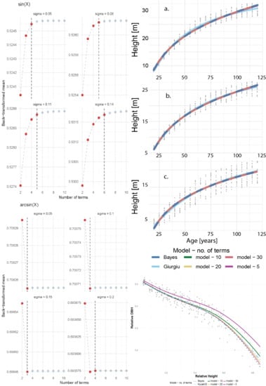
Convergence of sine transformation according to the number of terms in Taylor series expansion. The vertical dotted line identifies the number of terms for which two consecutive differences between Taylor series estimates are less than the preset value of the order of 10−5.
Figure 1.
Convergence of sine transformation according to the number of terms in Taylor series expansion. The vertical dotted line identifies the number of terms for which two consecutive differences between Taylor series estimates are less than the preset value of the order of 10−5.

Figure 2.
Convergence of the cosine transformation according to the number of terms in the Taylor series expansion. The vertical dotted line identifies the number of terms for which two consecutive differences between Taylor series estimates are less than the preset value of the order of 10−5.
Figure 2.
Convergence of the cosine transformation according to the number of terms in the Taylor series expansion. The vertical dotted line identifies the number of terms for which two consecutive differences between Taylor series estimates are less than the preset value of the order of 10−5.

Figure 3.
Convergence of the tangent transformation according to the number of terms in the Taylor series expansion. The vertical dotted line identifies the number of terms for which two consecutive differences between Taylor series estimates are less than the preset value of the order of 10−5.
Figure 3.
Convergence of the tangent transformation according to the number of terms in the Taylor series expansion. The vertical dotted line identifies the number of terms for which two consecutive differences between Taylor series estimates are less than the preset value of the order of 10−5.

Figure 4.
Convergence of the arcsine transformation according to the number of terms in the Taylor series expansion. The vertical dotted line identifies the number of terms for which two consecutive differences between Taylor series estimates are less than the preset value of the order of 10−5.
Figure 4.
Convergence of the arcsine transformation according to the number of terms in the Taylor series expansion. The vertical dotted line identifies the number of terms for which two consecutive differences between Taylor series estimates are less than the preset value of the order of 10−5.

Figure 5.
Convergence of the arccosine transformation according to the number of terms in the Taylor series expansion. The vertical dotted line identifies the number of terms for which two consecutive differences between Taylor series estimates are less than the preset value of the order of 10−5.
Figure 5.
Convergence of the arccosine transformation according to the number of terms in the Taylor series expansion. The vertical dotted line identifies the number of terms for which two consecutive differences between Taylor series estimates are less than the preset value of the order of 10−5.

Figure 6.
Convergence of the arctangent transformation according to the number of terms in the Table 1.
Figure 6.
Convergence of the arctangent transformation according to the number of terms in the Table 1.

Figure 7.
Convergence of the hyperbolic sine transformation according to the number of terms in the Taylor series expansion. The vertical dotted line identifies the number of terms for which two consecutive differences between Taylor series estimates are less than the preset value (order of 10−5).
Figure 7.
Convergence of the hyperbolic sine transformation according to the number of terms in the Taylor series expansion. The vertical dotted line identifies the number of terms for which two consecutive differences between Taylor series estimates are less than the preset value (order of 10−5).

Figure 8.
Convergence of the hyperbolic tangent transformation according to the number of terms in Table 1.
Figure 8.
Convergence of the hyperbolic tangent transformation according to the number of terms in Table 1.

Figure 9.
Site index modeling for the Norway spruce. An efficient Taylor series expansion contains at most 30 terms, irrespective of site productivity: a. class II (SI = 31.8 m) b. class III (SI = 26.9 m) c. class IV (SI = 21.9 m). The difference between the Bayesian models and the one based on Taylor series expansion is so minute that is visually undistinguishable.

Figure 10.
Taper modeling for the loblolly pine plantations from east Louisiana. An efficient Taylor series expansion contains five to 30 terms.
Figure 10.
Taper modeling for the loblolly pine plantations from east Louisiana. An efficient Taylor series expansion contains five to 30 terms.


Table 1.
Efficient Taylor series expansion converges according to the scree plot and to the preset value of 10−5. Mean and variance of ξ from Equation (1) mirror the values from Strimbu, Amarioarei, and Paun [29]. The values for mean are in radians. The expectation is the inverse of the transformation computed with Equations (2) and (3).
| Transformation | Mean | Variance | Expectation | Number of Terms | |
|---|---|---|---|---|---|
| Scree Plot | Preset Value | ||||
| Sine | 0.5 | 0.05 | 0.525 | 4 | 4 |
| 0.08 | 0.526 | 4 | 4 | ||
| 0.11 | 0.528 | 4 | 5 | ||
| 0.14 | 0.532 | 4 | 6 | ||
| Cosine | 0.5 | 0.05 | 1.045 | 4 | 4 |
| 0.08 | 1.042 | 4 | 4 | ||
| 0.11 | 1.042 | 4 | 5 | ||
| 0.14 | 1.039 | 5 | 6 | ||
| Tangent | 0.5 | 0.05 | 0.463 | 3 | 5 |
| 0.08 | 0.462 | 3 | 6 | ||
| 0.11 | 0.460 | 3 | 7 | ||
| 0.14 | 0.457 | 3 | 9 | ||
| Arcsine | π/4 | π/64 | 0.706 | 3 | 3 |
| π/32 | 0.704 | 3 | 3 | ||
| 3π/64 | 0.699 | 3 | 3 | ||
| π/16 | 0.694 | 3 | 4 | ||
| Arccosine | π/4 | π/64 | 0.706 | 3 | 3 |
| π/32 | 0.704 | 3 | 3 | ||
| 3π/64 | 0.699 | 3 | 3 | ||
| π/16 | 0.694 | 3 | 4 | ||
| Arctangent | π/8 | π/128 | 0.414 | 3 | 4 |
| π/64 | 0.415 | 3 | 5 | ||
| 3π/128 | 0.417 | 3 | 5 | ||
| π/32 | 0.419 | 3 | 5 | ||
| Hyperbolic sine | 0.5 | 0.05 | 0.481 | 3 | 4 |
| 0.08 | 0.480 | 3 | 5 | ||
| 0.11 | 0.479 | 3 | 5 | ||
| 0.14 | 0.478 | 3 | 6 | ||
| Hyperbolic tangent | 0.5 | 0.05 | 0.552 | 4 | 5 |
| 0.08 | 0.555 | 4 | 6 | ||
| 0.11 | 0.561 | 5 | 7 | ||
| 0.14 | 0.569 | 6 | 9 | ||
Table 2.
Comparison of the site index models for the Norway spruce (index age 100 years).
| Site Index Class | Model | Bias (%) | MAE (%) | RMSE (%) | Correlation Coefficient |
|---|---|---|---|---|---|
| IV (21.9 m) | Giurgiu-Draghiciu | −2.2 | 13.1 | 15.8 | 0.923 |
| Bayesian | −2.2 | 14.4 | 18.1 | 0.917 | |
| Parsimonious 10 terms | −2.2 | 14.4 | 18.1 | 0.917 | |
| Parsimonious 30 terms | −2.2 | 14.4 | 18.1 | 0.917 | |
| III (26.9 m) | Giurgiu-Draghiciu | −0.4 | 5.7 | 6.8 | 0.976 |
| Bayesian | −0.4 | 6.0 | 7.3 | 0.975 | |
| Parsimonious 10 terms | −0.4 | 6.0 | 7.3 | 0.975 | |
| Parsimonious 30 terms | −0.4 | 6.0 | 7.3 | 0.975 | |
| II (31.8 m) | Giurgiu-Draghiciu | −0.3 | 4.8 | 5.9 | 0.981 |
| Bayesian | −4.5 | 5.0 | 6.0 | 0.977 | |
| Parsimonious 10 terms | −4.5 | 5.0 | 6.0 | 0.978 | |
| Parsimonious 30 terms | −4.5 | 5.0 | 6.0 | 0.978 |
Table 3.
Comparison of the taper models for loblolly pine from east Louisiana.
| Measure | Parsimonious Model | Kozak– Model 02 | Bayesian Model | |
|---|---|---|---|---|
| 10-Terms | 30-Terms | |||
| Correlation coefficient | 0.961 | 0.964 | 0.980 | 0.960 |
| Bias (%) | −1.9 | −0.05 | −0.18 | 0.16 |
| MAE (%) | 5.0 | 4.4 | 3.2 | 4.5 |
| RMSE (%) | 8.4 | 7.8 | 3.8 | 8.2 |
© 2020 by the authors. Licensee MDPI, Basel, Switzerland. This article is an open access article distributed under the terms and conditions of the Creative Commons Attribution (CC BY) license (http://creativecommons.org/licenses/by/4.0/).
Share and Cite
MDPI and ACS Style
Amarioarei, A.; Paun, M.; Strimbu, B. Development of Nonlinear Parsimonious Forest Models Using Efficient Expansion of the Taylor Series: Applications to Site Productivity and Taper. Forests 2020, 11, 458. https://doi.org/10.3390/f11040458
AMA Style
Amarioarei A, Paun M, Strimbu B. Development of Nonlinear Parsimonious Forest Models Using Efficient Expansion of the Taylor Series: Applications to Site Productivity and Taper. Forests. 2020; 11(4):458. https://doi.org/10.3390/f11040458
Chicago/Turabian StyleAmarioarei, Alexandru, Mihaela Paun, and Bogdan Strimbu. 2020. "Development of Nonlinear Parsimonious Forest Models Using Efficient Expansion of the Taylor Series: Applications to Site Productivity and Taper" Forests 11, no. 4: 458. https://doi.org/10.3390/f11040458
Note that from the first issue of 2016, this journal uses article numbers instead of page numbers. See further details here.