Estimation of Above-Ground Carbon Storage and Light Saturation Value in Northeastern China’s Natural Forests Using Different Spatial Regression Models

Abstract

In recent years, accurate estimation and spatial mapping of above-ground carbon (AGC) storage in forests have been crucial for formulating carbon trading policies and promoting sustainable development strategies. Forest structure complexities mean that during their growth, trees may be affected by the surrounding environment, giving rise to spatial autocorrelation and heterogeneity in nearby forest segments. When estimating forest AGC through remote sensing, data saturation can arise in dense forest stands, adding to the uncertainties in AGC estimation. Our study used field-measured stand factors data from 138 forest fire risk plots located in Fenglin County in the Northeastern region, set within a series of temperate forest environments in 2021 and Sentinel-2 remote sensing image data with a spatial resolution of 10 m. Using ordinary least squares (OLS) as a baseline, we constructed and compared it against four spatial regression models, spatial lag model (SLM), spatial error model (SEM), spatial Durbin model (SDM), and geographically weighted regression (GWR), to better understand forest AGC spatial distribution. The results of local spatial analysis reveal significant spatial effects among plot data. The GWR model outperformed others with an R² value of 0.695 and the lowest rRMSE at 0.273, considering spatial heterogeneity and extending the threshold range for AGC estimation. To address the challenge of light saturation during AGC estimation, we deployed traditional linear functions, the generalized additive model (GAM), and the quantile generalized additive model (QGAM). AGC light saturation values derived from QGAM most accurately reflect the actual conditions, with the forests in Fenglin County exhibiting a light saturation range of 108.832 to 129.894 Mg/ha. The GWR effectively alleviated the impact of data saturation, thereby reducing the uncertainty of AGC spatial distribution in Fenglin County. Overall, accurate predictions of large-scale forest carbon storage provide valuable guidance for forest management, forest conservation, and the promotion of sustainable development strategies.

1. Introduction

Forests play a central and indispensable role in the global carbon cycle [1,2]. The forest ecosystem is characterized by species richness, structural complexity, and diverse resources [3]. The powerful carbon sequestration ability of forests plays a crucial role in climate change [4,5]. Forest above-ground carbon (AGC) storage is defined as the total amount of carbon stored in the above-ground components of a forest ecosystem, including tree trunks, branches, and leaves [6,7]. Forest AGC represents a more stable indicator of long-term carbon accumulation and is an essential attribute for reflecting the dynamics of forest ecosystems [8,9]. Although most studies indicate that estimating AGC in forests comes with uncertainty [10,11,12], accurately assessing its spatial distribution remains essential for climate change mitigation and shaping carbon trading policies [13].

According to convention, forest AGC estimation methods can be categorized into field measurement techniques based on allometric equations [14,15], detailed biophysical models [16,17], and empirical models that combine field data with various remote sensing data, including optical, thermal, microwave, radar, and LiDAR data [18]. The advantage of remote sensing technology lies in its ability to effortlessly collect information on forest types and coverage, facilitating large-scale, long-term, and repetitive monitoring [19,20]. As an economically efficient approach, it is widely employed for the extensive estimation of forest AGC [21]. Multisensory data have been widely used for AGC mapping and are a primary data source for AGC estimation [22,23]. However, the processing and analysis of multisensory data can pose complexities due to the diverse characteristics and calibration requirements of different sensors [24]. Furthermore, cost and feasibility considerations need to be accounted for when acquiring data. LiDAR data, unaffected by lighting conditions, offer high-precision estimation by capturing canopy height information. It is considered to be a promising technology for AGC estimation [25,26]. However, due to its high cost, the complexity of forest structure, and the challenges associated with data processing, LiDAR data are predominantly employed in small-scale areas. Optical remote sensing data are a commonly used data source for estimating AGC [27,28]. Medium-resolution and high-resolution data are usually used for local-scale AGC estimation, such as Landsat series, SPOT, Sentinel series, and GF series [11,29,30,31]. Despite the significant limitations of optical imagery, including relatively low estimation accuracy, lack of consistency, and significant initial costs to acquire and produce results, it still serves as an alternative method for mapping large-scale forest AGC [27]. High-resolution imagery can be used to gather more detailed vegetation information, such as vegetation indices and texture features [32,33,34]. These data sets are typically used for parametric or nonparametric estimation methods by establishing a complete mathematical model and combining remote sensing image information with ground standard survey data. Ultimately, analysis formulas are used to estimate AGC [35]. Compared to parametric models, nonparametric models generally exhibit superior data fitting ability and higher estimation accuracy [36,37]. However, nonparametric models are more susceptible to the size and representativeness of the sample, meaning that their effectiveness may be limited in study areas with smaller sample sizes [38]. As a result, addressing the challenge of reducing uncertainty in estimating forest AGC based on remote sensing data remains a significant area of research [11,38,39].

Differences in AGC levels are anticipated across different regions due to variations in geographic location, site conditions, soil characteristics, and climate [40]. Vegetation types and their structures and physiologies are influenced to varying degrees by the surrounding environment during the growth process, which is manifested in forestry data as spatial correlations between adjacent trees. As trees compete, spatial heterogeneity becomes evident [41]. Although the spatial distribution of trees is discrete and independent variable data, their spatial distribution at the stand level, such as diameter at breast height and tree height, is directly affected by different continuous variables, such as light conditions, soil characteristics, temperature, and rainfall, so it can be assumed that these variables are continuous and spatially correlated [42]. Some scholars believe that spatial effects consist of spatial heterogeneity and spatial autocorrelation. Ignoring spatial effects in the modeling process may result in biased tests and suboptimal predictive models [43]. The spatial regression model can incorporate spatial effects into the regression model without requiring independent data [38,44]. Among the most commonly used models are the spatial lag model (SLM), the spatial error model (SEM), and the spatial Durbin model (SDM), which aim to capture the spatial dependence and autocorrelation of data [45,46,47]. However, when dealing with spatial heterogeneity, the geographically weighted regression (GWR) model is the preferred approach. GWR allows for a local analysis of the relationship between variables, providing more accurate and detailed results in situations where the relationship between variables differs spatially [48]. The use of remote sensing to determine the spatial distribution of forest AGC and the challenge of reducing estimation uncertainty have gained widespread attention, especially the prevalent issues of overestimation and underestimation [49,50]. When the forest cover on the ground is too dense to be accurately distinguished by remote sensing methods, a data saturation phenomenon may occur.

This study focuses on the mixed coniferous forest AGC of a 2967 km² area in Fenglin County, Yichun City, Heilongjiang Province, Northeast China. It aims to offer a reference for estimating forest AGC in the Northeastern Forest Region. Using Sentinel-2 remote sensing images and 138 field-measured plots, both nonspatial and spatial regression models were employed to evaluate their capabilities in estimating forest AGC. The study contents and methods are described as follows: (1) we calculate the forest AGC storage using field measurements and remote sensing imagery processing and subsequently select modeling variables through stepwise regression analysis; (2) we construct ordinary least squares models and spatial regression models and compare their predictive abilities; (3) we analyze the inversion and spatial distribution of forest AGC in the study area; and (4) finally, we calculate AGC light saturation values resulting from data saturation phenomena during remote sensing estimation. The objective of this study is to use remote sensing technology to accurately estimate the spatial distribution of above-ground carbon storage in temperate forests, offering guidance and direction for forest dynamic monitoring. Additionally, it explores how various spatial regression models can enhance the estimation accuracy of forest AGC and alleviate challenges posed by data saturation.

2. Materials and Methods

2.1. Study Area

The study area is in Fenglin County, Yichun City, Heilongjiang Province, Northeast China, and includes the three forestry bureaus of Wuying, Hongxing, and Xinqing. It is situated on the southern slope of the Xiaoxing’an Mountains and serves as a quintessential example of the Northeastern Forest Zone. The Northeastern Forest Zone is an ecologically significant region in China, playing a pivotal role in timber production, biodiversity conservation, and maintaining environmental stability. The specific geographical location is shown in Figure 1. This area has a north temperate continental humid monsoon climate, with an annual average temperature of 0.6 °C and an annual precipitation of 500–610 mm [51]. Most of the precipitation is concentrated in June–August, which accounts for 73% of the total annual precipitation. The annual temperature variation range of the study site spans from −34 °C to 33 °C, and the average annual sunshine duration is approximately 2196 h. Historical meteorological data were sourced from the China National Meteorological Information Center (http://data.cma.cn/ (accessed on 15 April 2023)). This area is a natural forest, and the main vegetation types are mixed coniferous and broad-leaved forests, deciduous broad-leaved forests, and temperate coniferous forests. The dominant tree species include Pinus, Betula, Larix, Picea, Abies, Fraxinus, and Populus. This region has abundant diverse forest resources and is a national-level nature reserve. It contains the most representative forest type in Northeast China—coniferous and broad-leaved mixed forest dominated by Korean pine.

2.2. Data Acquisition and Treatment

2.2.1. Processing Standard Ground Survey Data

Standard ground survey data were sourced from 138 fixed distribution sample plots for forest fire risk investigation in Fenglin County in 2021. Each sample plot had an area of 0.06 ha, which translates to 600 m² or a square that is approximately 20 m × 30 m. The specific distribution locations of the sample plots are shown in Figure 1b.

The survey of the sample plot comprises various factors, such as the average diameter at breast height, average tree height, number of trees, forest age, vegetation type, and dominant tree species. Specifically, the DBH of the tree was measured using diameter tape, and the tree height and crown base height were measured with an ultrasonic altimeter. In addition, we also measured the location within the plot and the geographic coordinates of all trees using real-time kinematic (RTK) technology and Global Navigation Satellite System (GNSS) receivers. We use GNSS receivers to obtain the coordinates of the center point and four corner points of the sample plots. An example of a sample plot is shown in Figure 2.

The calculation of forest above-ground biomass (AGB) followed prior research on forest carbon storage in the Xiaoxing’an Mountains [52]. The AGB of individual trees for different tree species was calculated using the individual tree biomass model from the DBH data collected from each tree measured, as shown in Equations (1)–(3). The calculated values of W_S, W_B, and W_L were multiplied by the corresponding carbon content coefficients provided in

Table 1. Carbon storage conversion coefficients of different tree species in the Xiaoxing’an Mountains. (Num is the number of samples; SD is the standard deviation.)

Species	Carbon Storage Conversion			Num	SD
	CS	CB	CL
Picea koraiensis Nakai	0.4727	0.4875	0.4839	48	0.0407
Abies fabri (Mast.) Craib	0.4673	0.4783	0.5057	60	0.0406
Tilia amurensis Rupr.	0.4426	0.4255	0.4484	46	0.0212
Quercus mongolica	0.4558	0.4491	0.4672	64	0.0201
Ulmus pumila	0.4355	0.433	0.4322	40	0.0183
Acer pictum Thunb.	0.4422	0.4346	0.4462	46	0.0187
Betula dahurica Pall.	0.4529	0.4585	0.4639	52	0.0179
Betula platyphylla	0.4634	0.4619	0.4857	73	0.0229
Populus davidiana Dode	0.4430	0.4454	0.4587	54	0.0193
Pinus sylvestris var. mongolica	0.4775	0.4833	0.4967	85	0.0203
Pinus koraiensis Sieb. et Zucc	0.4807	0.4989	0.4924	34	0.0108
Larix gmelinii	0.4695	0.4761	0.4832	103	0.0311

to obtain C_S, C_B, and C_L respectively. Finally, Equation (4) was used to calculate the AGC of a single tree. The sum of the AGC of individual trees in each plot divided by the unit area is the AGC of each plot, and the unit used is Mg/ha.

$$W_S{=C}_0\ast D^{b_0}/\left({1+r}_2\ast D^{k_2}{+r}_3\ast D^{k_3}{+r}_4\ast D^{k_4}\right)$$

(1)

$$W_B{=r}_2\ast C_0\ast D^{\left(k_2{+b}_0\right)}/\left({1+r}_2\ast D^{k_2}{+r}_3\ast D^{k_3}{+r}_4\ast D^{k_4}\right)$$

(2)

$$W_L{=r}_3\ast C_0\ast D^{\left(k_3{+b}_0\right)}/\left({1+r}_2\ast D^{k_2}{+r}_3\ast D^{k_3}{+r}_4\ast D^{k_4}\right)$$

(3)

where W_S is the AGB of a single wood trunk; W_B is the AGB of single wood branches; W_L is the AGB of single wood leaves; D is tree diameter at breast height; and c₀, b₀, r₂, k₂, r₃, k₃, r₄, and k₄ are the biomass model parameters of different tree species.

$${C=C}_S{+C}_B{+C}_L$$

(4)

where C is the AGC of a single tree; C_S is the AGC of a single tree trunk; C_B is the AGC of single tree branches; and C_L is the AGC of single tree leaves.

2.2.2. Remote Sensing Data

Sentinel-2 is a large-scale, high-resolution multispectral imaging satellite funded by the European Union, the European Space Agency (ESA), and the Copernicus program. It is primarily used for monitoring the land environment and can provide observations on land vegetation growth, land cover status, and inland waterways and coastal areas. The remote sensing data used in the study were Sentinel-2 Level-2A images acquired in April 2021, with image IDs N0300_R046_T52UEU and N0300_R046_T52UDU. To ensure data quality, the selected images over the study area were free of cloud cover. Level-2A images have undergone orthorectification, subpixel-level geometric accuracy correction, radiometric calibration, and atmospheric correction [53]. The remote sensing images are all downloaded from the Google Earth Engine platform (https://earthengine.google.com/platform/ (accessed on 2 March 2022)). The original remote sensing imagery consists of 12 bands. In this study, we only used bands with a resolution of 10 m, specifically band 2 (blue band: 0.458–0.523 μm), band 3 (green band: 0.543–0.578 μm), band 4 (red band: 0.650–0.680 μm), and band 8 (near-infrared band: 0.785–0.900 μm). In order to ensure that the pixel area of the remote sensing image matches that of the measured sample plot area, we employed the nearest neighbor interpolation method to resample the remote sensing image to a spatial resolution of 25 m. Subsequently, we used ENVI 5.3 software to crop the remote sensing image of the study area and to compute various remote sensing factors, including the original bands, vegetation indices, and texture features [54,55,56,57,58]. We computed the co-occurrence matrices for only the red, green, blue, and near-infrared bands, resulting in a total of 32 texture features. The corresponding formulas are shown in

Table 2. The calculation method of the vegetation index (B1, B2, B3, and B4 represent blue reflectivity, green reflectivity, red reflectivity, and near-infrared reflectivity, respectively).

Type	Vegetation Index	Abbreviation	Calculation Formula
Original Band	B2-Blue	B1	B2
	B3-Green	B2	B3
	B4-Red	B3	B4
	B8-NIR	B4	B8
Vegetation Index	Ratio Vegetation Index	RVI	B8/B4
	Atmospheric Ratio Vegetation Index	ARVI	[B8 − (2 × B4 − B2))/(B8 + (2 × B4 − B2)]
	Soil Adjusted Vegetation Index	SAVI	1.5 × (B8 − B4)/8 × (B8 + B4 + 0.5)
	Difference Vegetation Index	DVI	B8 − B4
	Normalized Difference Vegetation Index	NDVI	(B8 − B4)/(B8 + B4)
	Weighted Difference Vegetation Index	WDVI	B8 − 0.5 × B4
	Infrared Percentage Vegetation Index	IPVI	B8/(B8 + B4)
	Red–Green Vegetation Index	RGVI	(B4 − B3)/(B4 + B3)
	Triangular Vegetation Index	TVI	0.5 × [120 × (B8 − B3)] − 200 × (B4 − B3)
	Visible Atmospheric Resistance Index	VARI	(B3 − B4)/(B3 + B4 − B2)
Texture	Mean	ME	$\sum _{i=0}^{N-1}\sum _{j=0}^{N-1}iP\left(i,j\right)$
	Variance	VA	$\sum _{i=0}^{N-1}\sum _{j=0}^{N-1}{\left(i-mean\right)}^{2}P\left(i,j\right)$
	Homogeneity	HO	$\sum _{i=0}^{N-1}\sum _{j=0}^{N-1}\frac{P\left(i,j\right)}{1+{\left(i-j\right)}^2}$
	Dissimilarity	CO	$\sum _{\left|i-j\right|=0}^{N-1}{\left|i-j\right|}^2\left\{\sum _{i=0}^N\sum _{j=0}^{N}P\left(i,j\right)\right\}$
	Contrast	DI	$\sum _{\left|i-j\right|=0}^{N-1}\left|i-j\right|\left\{\sum _{i=0}^N\sum _{j=0}^{N}P\left(i,j\right)\right\}$
	Entropy	EN	$-\sum _{i=0}^{N-1}\sum _{j=0}^{N-1}P\left(i,j\right)log\left(P\left(i,j\right)\right)$
	Angular Second Moment	ASM	$\sum _{i=0}^{N-1}\sum _{j=0}^{N-1}P{\left(i,j\right)}^2$
	Correlation	COR	$\frac{{\sum }_{i=0}^{N-1}{\sum }_{j=0}^{N-1}P{\left(i,j\right)}^2-{\mathsf{\mu }}_x{\mathsf{\mu }}_y}{{\sigma }_x{\sigma }_y}$

. Texture features derived from remote sensing imagery capture the visual homogeneity or heterogeneity within the image. These features represent specific variations in color or grayscale on the Earth’s surface and are often indicative of the inherent properties of the surface objects [59,60,61]. Texture features provide image horizontal structure information and reflect the spatial variation in its gray values. When combined with vegetation indices, they can effectively depict the characteristics and changes in land features. In this study, terrain factors were extracted using a free digital elevation model (DEM). Downloaded from the Geospatial Data Cloud website (https://www.gscloud.cn/search (accessed on 19 March 2022)), ArcGIS 10.7 with the spatial and statistical analyst extensions was used to extract terrain factors, such as elevation, slope, and aspect.

The Kolmogorov–Smirnov (K-S) test was used to check the normality of the research data. Then, the Pearson correlation was applied to study the relationship between AGC and factors such as forest stand, terrain, and remote sensing in the study area. Multiple stepwise regression analysis (MSR) was used to select the dependent variables for AGC modeling, with the significance levels for variable entry and removal set at 0.1 and 0.05, respectively. Variables were determined for collinearity based on a standard of variance inflation factor (VIF) of less than 10. Finally, utilizing the selected remote sensing variables through stepwise regression, we performed AGC estimation and spatial distribution analysis.

2.3. Model Building and AGC Estimation

2.3.1. Ordinary Least Squares Model

The ordinary least squares (OLS) model is used to obtain a best-fit model by incorporating data and prior information [62]. The dependent variable Y is the AGC, with n observations and p independent variables X, such as forest, terrain, and remote sensing factors. The relationship between the independent variable X and the dependent variable Y can be expressed using linear regression, as shown in Equation (5):

$$Y=X\beta +\epsilon$$

(5)

where $\beta$ is the model parameter and $\epsilon$ is the model residual, which are assumed to follow a distribution. The parameters are estimated using the least sum of squares of the deviations between the dependent variable and the predicted values.

The OLS model is based on assumptions that apply to a whole region and is a global model where the constant and coefficients of explanatory variables are assumed to be the same across different study areas. However, the OLS model does not account for spatial autocorrelation and spatial heterogeneity between different regions.

2.3.2. Spatial Lag Model

The spatial lag model (SLM), also known as the spatial autoregressive model, is an autoregressive model that account for spatial variables [63]. When the dependent variable has significant spatial dependence on a spatial point, the spatial lag item can be introduced as a new explanatory variable in the classical statistical regression model. Assuming that the AGC of a sampling site is influenced by surrounding sampling sites, each sampling site can be viewed as a lagged effect of other sampling sites [64]. The SLM model is realized by adding the spatial lag item of the dependent variable y to the OLS model, as shown in Equation (6):

$${Y=X\beta +\rho W}_y+\epsilon$$

(6)

where $\beta$ is the prognostic parameter; W is the row-normalized spatial weight matrix; $W_y$ is the weighted average of adjacent sample sites; y is the spatial lag item; $\rho$ is the spatial autocorrelation parameter, which is influenced by the matrix W; and $\epsilon$ is a random error item that obeys an $N\left({0,\sigma }^{2}I\right)$ normal distribution.

2.3.3. Spatial Error Model

The spatial error model (SEM) refers to a model where the error term is spatially correlated, meaning that the spatial correlation is attributed to the error term rather than the systematic part of the model [65]. The SEM assumes that the spatial autocorrelation is considered from the error term without changing the explanatory variables, thereby estimating the spatial autocorrelation coefficient. Specifically, the model error is partitioned into two components: the error caused by spatial autocorrelation and the error from the model itself, as shown in Equation (7).

$${Y=X\beta +\lambda W}_{\epsilon }+\xi$$

(7)

where $\lambda$ is the spatial autocorrelation parameter; $W_{\epsilon }$ is the spatial error term; and $\xi$ is a random error item that obeys an $N\left({0,\sigma }^{2}I\right)$ normal distribution.

2.3.4. Spatial Durbin Model

The spatial Durbin model (SDM) is an extended form that combines the SLM and SEM by incorporating corresponding constraints on these models [66]. This model considers the spatial autocorrelation of both the dependent and independent variables and can be formulated as shown in Equation (8).

$$Y=\rho WY+X\beta +\lambda \rho WX\beta +\epsilon$$

(8)

where $\rho$ is the spatial autoregressive coefficient, which indicates the strength of spatial dependence. W is the spatial weight matrix, which describes the degree of spatial interdependence in the sample. $\lambda$ is the spatial lag coefficient, and $\rho WY$ and $\lambda \rho WX\beta$ denote the spatially lagged dependent and independent variables, respectively.

2.3.5. Geographically Weighted Regression Model

The geographically weighted regression model (GWR) is widely recognized as one of the most effective methods for addressing spatial heterogeneity [44,67]. This model extends the global regression model by building a regression model at each point in space, weighting all observations using a distance function from nearby points [68]. The aim is to identify spatial patterns by estimating a set of coefficient values for each point by moving a window over the data [69]. The basic form of the model is shown in Equation (9).

$$Y_{\left(u_i{,v}_i\right)}{=\beta }_{0\left(u_i{,v}_i\right)}{+\beta }_{1\left(u_i{,v}_i\right)}{X}_{1i}{+\beta }_{2\left(u_i{,v}_i\right)}{X}_{2i}+\cdots {+\beta }_{n\left(u_i{,v}_i\right)}{X}_{ni}{+\epsilon }_i$$

(9)

where $\left(u_i{,v}_i\right)$ is the coordinate at point i; $Y_{\left(u_i{,v}_i\right)}$ is the dependent variable at point i; n is the number of samples; $X_{ni}$ is the value of the nth variable at point i; ${\beta }_0$ is the intercept; and ${\epsilon }_i$ is the error term. In this model, the parameters of each sampling point are estimated based on the spatial weight matrix (W_i), where W_i is a diagonal matrix of spatial weights for point i, and $W_i=f\left(d_i,h\right)$, where $d_i$ is the distance vector between location i and all neighbors and h is the bandwidth. We used an adaptive bisquare kernel function to select the optimal bandwidth, enabling the detection of nonstationary relationships that global models might overlook.

2.3.6. Model Accuracy Evaluation Method

The sample plots are divided into 103 training data sets and 35 testing data sets by random sampling, and RStudio 4.2.1 is employed to fit OLS, SEM, SLM, SDM, and GWR models. The model fitting accuracy is commonly evaluated using the correlation coefficient (R²), the adjusted coefficient of determination ($R_{adj}^2$), the relative root mean squared error (rRMSE), the mean absolute percentage error (MARE), the mean absolute error (MAE), and the mean percentage bias (MPE) [70]. Typically, a higher R² and $R_{adj}^2$, as well as a lower rRMSE, MARE, MAE, and MPE, indicate better performance of the model. These statistical analyses are expressed in Equations (10)–(15).

$$R^2=1-\frac{{\sum }_{i=1}^n{\left(y-{\widehat{y}}_i\right)}^2}{{\sum }_{i=1}^n{\left(y-{\overline{y}}_i\right)}^2}$$

(10)

$$R_{adj}^2=1-\frac{\left(1-R^2\right)\left(n-1\right)}{n-k-1}$$

(11)

$$\mathrm{rRMSE}=\sqrt{\frac{\frac{1}{n}{\sum }_{i=1}^n{\left(y-{\widehat{y}}_i\right)}^2}{\overline{y}}}\times 100\%$$

(12)

$$\mathrm{MARE}=\frac{1}{n}{\sum }_{i=1}^n\frac{\left|y-{\widehat{y}}_i\right|}{y_i}$$

(13)

$$\mathrm{MAE}=\frac{1}{n}{\sum }_{i=1}^n \left|y-{\widehat{y}}_i\right|$$

(14)

$$\mathrm{MPE}=\frac{{\sum }_{i=1}^n\left|y-{\widehat{y}}_i\right|}{{\sum }_{i=1}^n{y}_i}\times 100\%$$

(15)

In this study, we analyzed spatial autocorrelation and heterogeneity in forest AGC and model residuals using global and local Moran’s I methods [71,72], as shown in Equation (16). A positive Moran’s I indicates similar residual levels, while a negative value suggests contrasting trends. If Moran’s I is near zero, the residuals are randomly distributed with no mutual influence [73,74]. Moran’s I was used to measure the global autocorrelation between the AGC and model prediction residuals.

$$\mathrm{I}=\frac{n{\sum }_{i=1}^n{\sum }_{j=1}^n{w}_{ij}\left(d\right)\left(x_i-\overline{x}\right)\left(x_j-\overline{x}\right)}{{\sum }_{i=1}^n{\sum }_{j=1}^n{w}_{ij}\left(d\right){\sum }_{i=1}^n{\left(x_i-\overline{x}\right)}^2}$$

(16)

where n is the sample size, $x_i$ is the observed values at different locations, $\overline{x}$ is the average of the observed values at different locations, and $w_{ij}\left(d\right)$ is the weight based on the distance between sample points i and j. The Z value is a multiple of the standard deviation, and the significance of Moran’s I is tested by the Z value to determine whether the spatial autocorrelation of the observed values exists. The Z value calculation method is shown in Equation (17).

$$\mathrm{Z}\left(\mathrm{I}\right)=\frac{\mathrm{I}-\mathrm{E}\left(\mathrm{I}\right)}{\sqrt{\mathrm{Var}\left(\mathrm{I}\right)}}$$

(17)

If the Z value falls within the range of −1.96 to +1.96, the uncorrected p value will be greater than 0.05. Therefore, the null hypothesis cannot be rejected, indicating that the spatial distribution of AGC is likely to be random and does not exhibit any spatial effects. If the Z value falls outside this range, the spatial pattern displayed would be a statistically significant cluster or dispersion trend [75]. Lastly, we used the local spatial autocorrelation tool in ArcGIS 10.7 to visualize the spatial cluster or dispersion trend [76].

2.3.7. Confirmation of Light Saturation Value

Optical remote sensing images can capture the unique spectral characteristics of different vegetation types. When the forest cover on the ground is too dense to be accurately distinguished by remote sensing methods, a data saturation phenomenon may occur. Since different remote sensing images and different estimation methods will produce different saturation values, this study defines the saturation value of light as a range, indicating that when the AGC reaches this range, using remote sensing images for AGC estimation will result in saturation. Previous studies on the saturation value of above-ground carbon storage often used the most relevant variables to build nonlinear or spherical models and calculated the extreme values as the saturation value of above-ground carbon storage [11]. However, using a single variable to estimate the saturation of above-ground carbon storage may result in the loss of valuable information, leading to low and inaccurate precision. The generalized additive model (GAM) is an additive modeling technique in which the predictor variables are modeled by a smoothing function [77]. This approach is highly flexible and offers strong interpretability. The quantile generalized additive model (QGAM) is based on the GAM, employing quantile regression for predictions. Compared to traditional methods, this approach can use more variables and avoid information loss. This study attempts to estimate the AGC saturation value using linear, quadratic, and logarithmic functions and GAM and QGAM. QGAM is fitted using seven quantile points (q = 0.2, 0.3, 0.4, 0.5, 0.6, 0.7, 0.8) to estimate the AGC saturation value in Fenglin County using range values to replace single-point values and eliminate estimation errors caused by maximum and minimum values. Unlike traditional regression models that only focus on the mean, QGAMs allow us to model in different distribution regions of the data, thus gaining a more comprehensive understanding of the nature of the data. The GAM and QGAM are fitted using functions from the gam and qgam packages in R [78] Figure 3 shows a flowchart of the steps used in our study.

3. Results

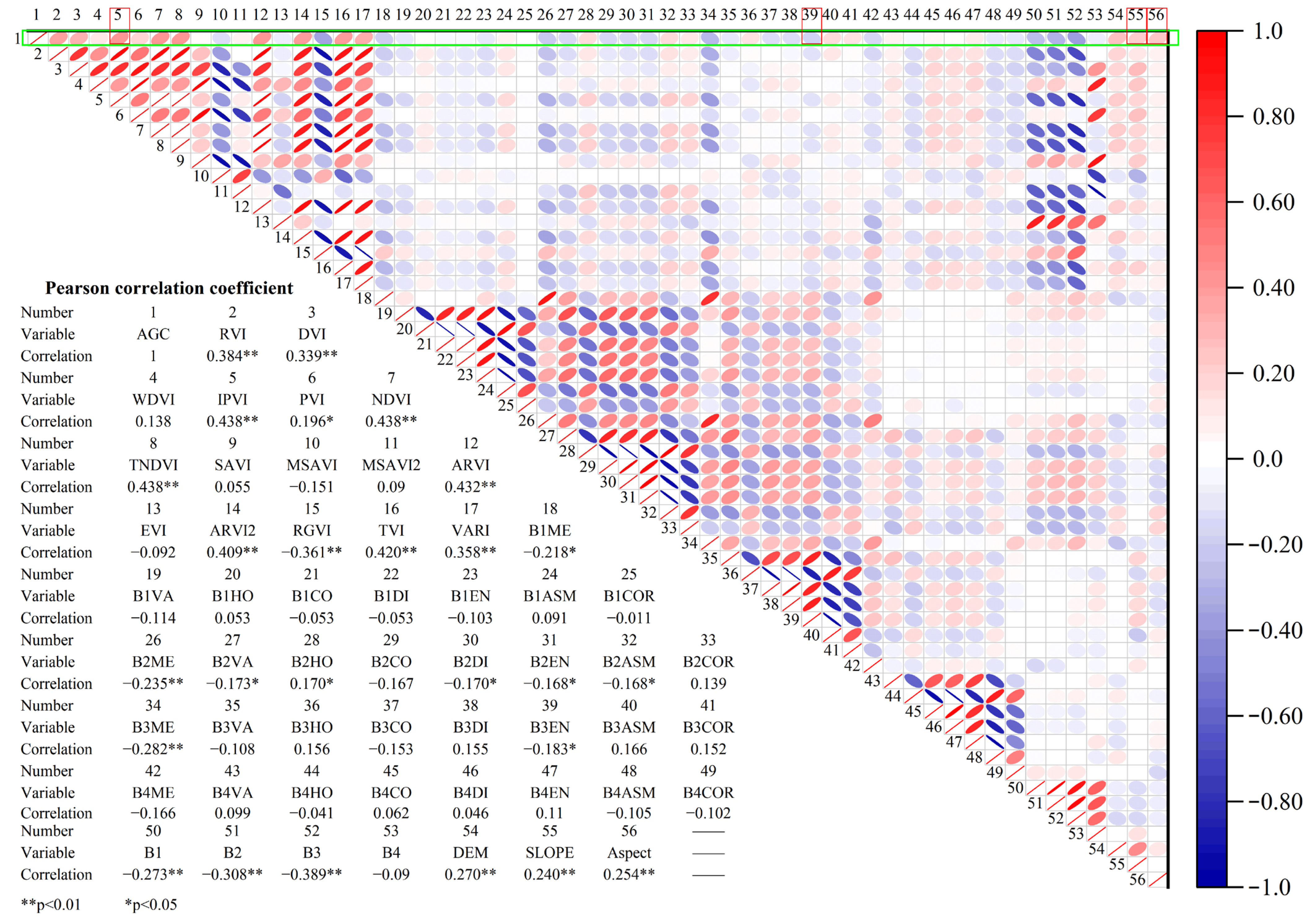
3.1. Variable Screening

Descriptive statistics for the data are shown in

Table 3. Descriptive statistics of independent variables and remote sensing variables. D: Kolmogorov–Smirnov distance; P: Kolmogorov–Smirnov test p-value.

Variable	Num	Min	Median	Max	Mean	Unit	Std	VIF	D	p
AGC	138	6.130	57.375	153.058	63.121	Mg/ha	30.951	―	0.090	0.213
IPVI	138	0.582	0.774	0.895	0.769	―	0.067	1.074	0.091	0.207
B3EN	138	0.000	0.349	1.581	0.502	―	0.472	1.087	0.108	0.964
SLOPE	138	0.155	4.787	15.133	5.494	°	3.570	1.098	0.118	0.927
Aspect	138	0.000	168.368	347.005	170.557	°	96.123	1.022	0.176	0.571

. Based on the K-S test results, as the null hypothesis assumes no difference between the data and a normal distribution, and with a p-value significantly greater than 0.05, we cannot reject the null hypothesis, indicating that the data can be considered to follow a normal distribution. According to the correlation analysis between AGC and remote sensing factors shown in Figure 4, 26 remote sensing factors exhibit a significant correlation at the p < 0.05 level. A stepwise regression method was used for optimal variable selection, and finally, four remote sensing variables, IPVI, B3EN, SLOPE, and Aspect, were selected to estimate and analyze the spatial distribution of AGC in Fenglin County. The mean AGC measured in the sample plot is 63.121 Mg/ha, which is attributed to the natural secondary forest being in the middle-aged stage. Due to the presence of a few trees with a diameter at breast height greater than 0.3 m in some plots, the AGC in those areas exhibits higher values, where peak value reaches up to 153.058 Mg/ha. All VIF values are below 10, indicating the absence of multicollinearity among the selected variables. This aids in achieving a stable, interpretable, and accurate model outcome, thereby preventing overfitting.

In the field of geography and spatial data analysis, the instability of the relationship between spatially distributed variables is called spatial nonstationarity. To study the spatial nonstationarity of different variables and AGC, a scatter diagram of AGC and different variables in space is shown in Figure 5. The distribution of AGC is lower in the central part of the study area, and each variable shows different trends as latitude and longitude increase. The distribution of IPVI closely mirrors that of AGC, both exhibiting a trend where values are elevated at the periphery of the study area while diminishing towards the central region.

3.2. Spatial Correlation Analysis

The independent variables selected after the stepwise regression were standardized, and Moran’s I test of spatial correlation was carried out on OLS. The results in

Table 4. Moran’s I test for spatial correlation in residuals.

Moran’s I	Moran’s I Statistic	Marginal Probability	Mean	Standard Deviation
0.8590	53.0058	0.0000	−0.0004	0.0162

show that the p-value is close to zero, indicating that there is significant spatial autocorrelation in the residuals of the OLS model. Therefore, when constructing the AGC model of Fenglin County, it is necessary to consider the spatial effect and solve the AGC estimation error caused by the spatial effect.

Using local spatial correlation analysis to explore the spatial distribution of various types of clusters, Figure 6 shows the cluster distribution of AGC. Spatial correlation refers to the phenomenon where objects that are close to each other spatially tend to have similar trends and values in their attributes. Conversely, if objects that are spatially close have different trends and values in their attributes, this spatial correlation manifests as a negative spatial correlation, which is characterized by the presence of a “high–high cluster” or “high–low outlier” distribution [79,80].

Table 5. Z score statistics of local Moran’s I. LH: low–high outlier; HL: high–low outlier; HH: high–high cluster; LL: low–low cluster.

Z Score	Type	Number	Percentage
<−2.58	LH	1	0.725%
−2.58~−1.96	HL	3	2.174%
−1.96~−1.65	―	0	0.000%
−1.65~1.65	―	115	83.333%
1.65~1.96	HH	8	5.797%
1.96~2.58	LL	10	7.246%
>2.58	LL	1	0.725%

shows the Z-score statistics for local Moran’s I. In the study area, there is one sample plot showing a low–high outlier, possibly due to its proximity to a road. There are three plots of land that show high–low outliers, which account for 2.174% of the total sample. Additionally, there are eight plots of land that exhibit high–high clustering, representing 5.797% of the total sample and showing a clear positive correlation. Finally, there are eleven plots of land that display low–low clustering, which account for 7.971% of the total sample.

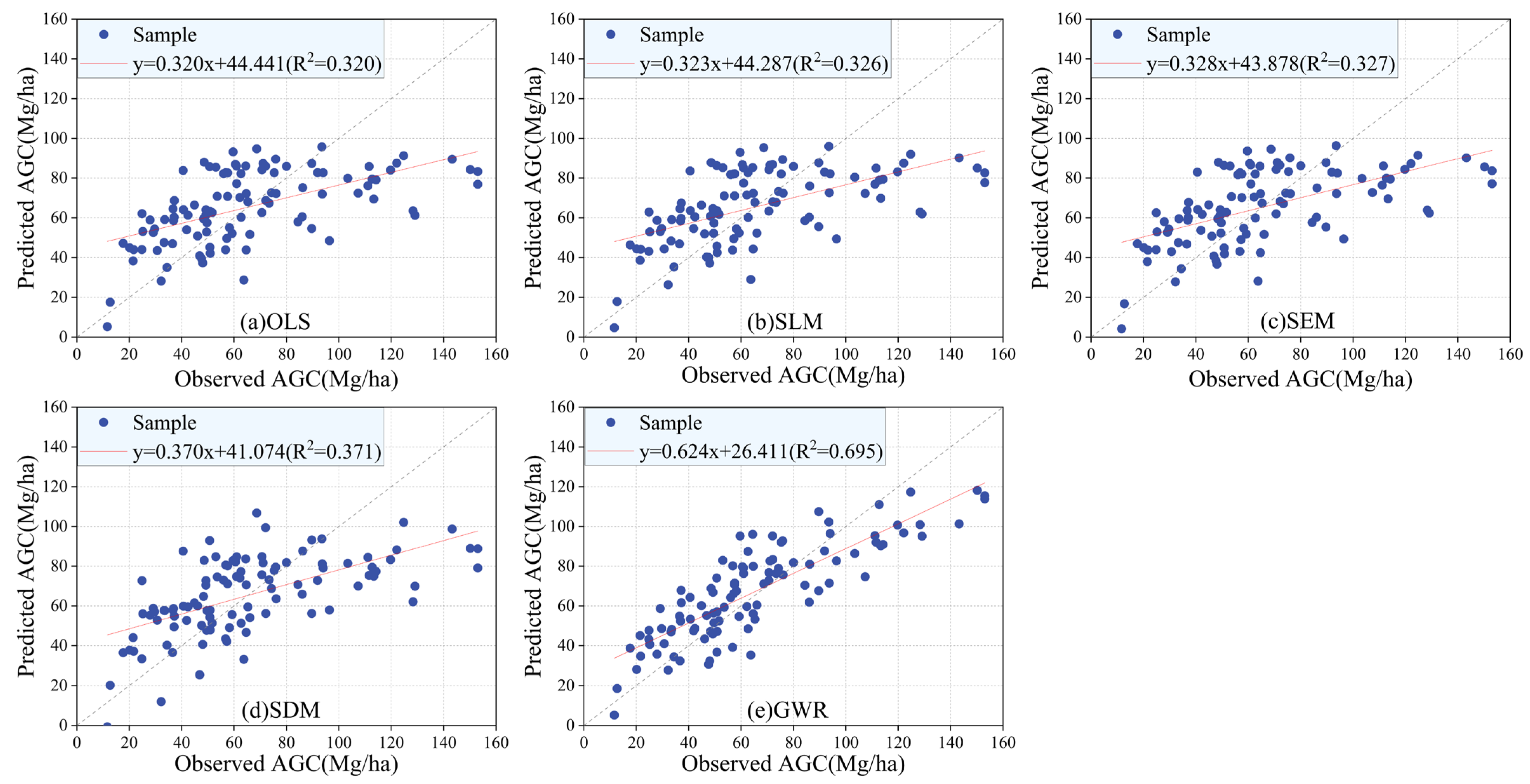
3.3. AGC Model Evaluation

The accuracy evaluation and prediction effect of each model are shown in

Table 6. Comparison of modeling results.

Models	Training Set (n = 103)						Validation Set (n = 35)
	R2	${\mathbf{R}}_{\mathbf{adj}}^2$	rRMSE (%)	MARE (Mg/ha)	MAE (Mg/ha)	MPB (%)	rRMSE (%)	MARE (Mg/ha)	MAE (Mg/ha)	MPB (%)
OLS	0.320	0.299	40.813	0.385	21.367	32.694	41.167	0.544	18.384	32.509
SLM	0.326	0.306	40.623	0.385	21.302	32.594	41.035	0.543	18.381	32.504
SEM	0.327	0.306	40.617	0.385	21.346	32.662	40.983	0.540	18.337	32.427
SDM	0.371	0.352	39.251	0.379	20.591	31.506	39.184	0.522	18.407	32.551
GWR	0.695	0.686	27.329	0.280	14.858	22.734	28.927	0.394	13.908	24.595

. The fitting effect and predictive ability of the OLS model are poor, and the SDM model performs best in the global regression model, which indicates that the SDM model can better fit the global structure of the data. The GWR model has the highest R² (0.695) and the smallest rRMSE (27.329), MARE (0.280), MAE (14.858), and MPB (22.734) values. To further visualize the model fitting performance, Figure 7 shows scatter plots of the observed and predicted AGC for 103 plots based on the OLS model and 4 spatial regression models. The global regression models exhibit a clear tendency to overestimate at low values and underestimate at high values of AGC when it is less than 40 Mg/ha or greater than 100 Mg/ha. The GWR estimation threshold of forest AGC was expanded from 0–100 Mg/ha to 0–120 Mg/ha. The GWR model not only offers superior predictive accuracy but also outperforms the other four global regression models in both fitting and predictive performance.

Furthermore, according to the variance analysis results of the GWR model shown in

Table 7. Variance analysis of the GWR model. Sum Sq: sum of squares of mean deviations; DF: degree freedom; Mean Sq: mean square; F: value of F.

Source	Sum Sq	DF	Mean Sq	F
OLS Model Residuals	73,278.508	98.000	―	―
GWR Model Improvement	33,306.914	40.442	823.571	―
GWR Model Residuals	39,971.593	57.558	694.458	1.186

, the GWR model has improved compared to the OLS model. The sum of squared residuals decreased by 33,306.914, indicating a decrease in the overall variation in the model residuals. The degrees of freedom also decreased by 40.442, and the mean squared residuals decreased by 823.571. These findings suggest that the OLS model had significant spatial autocorrelation and spatial heterogeneity in the residuals, while the GWR model could address the spatial effects present in the model residuals.

Figure 8 shows the spatial distribution of AGC in Fenglin County based on five different model inversions. This observation suggests a lower distribution of AGC in the central region, contrasting with a higher distribution in the southwestern region. This finding is consistent with the results of the high–high clustering discussed in Section 3.2. The OLS model tends to overestimate low values and underestimate high ones. While global regression improves estimation slightly, the GWR model significantly enhances the accuracy for both high and low value areas, aligning more closely with the true AGC distribution. The AGC distribution in Fenglin County exhibits a pattern of gradual increase from the sparser central region to the outer periphery, with areas of 100–120 Mg/ha encompassing 10.40% and those surpassing 120 Mg/ha occupying 3.99% of the total area. By using remote sensing information extracted from Sentinel-2 images and estimating the distribution of AGC in Fenglin County through a spatial regression model, the results obtained are consistent with the actual situation, providing a reference for analyzing the spatial distribution of forest AGC using remote sensing.

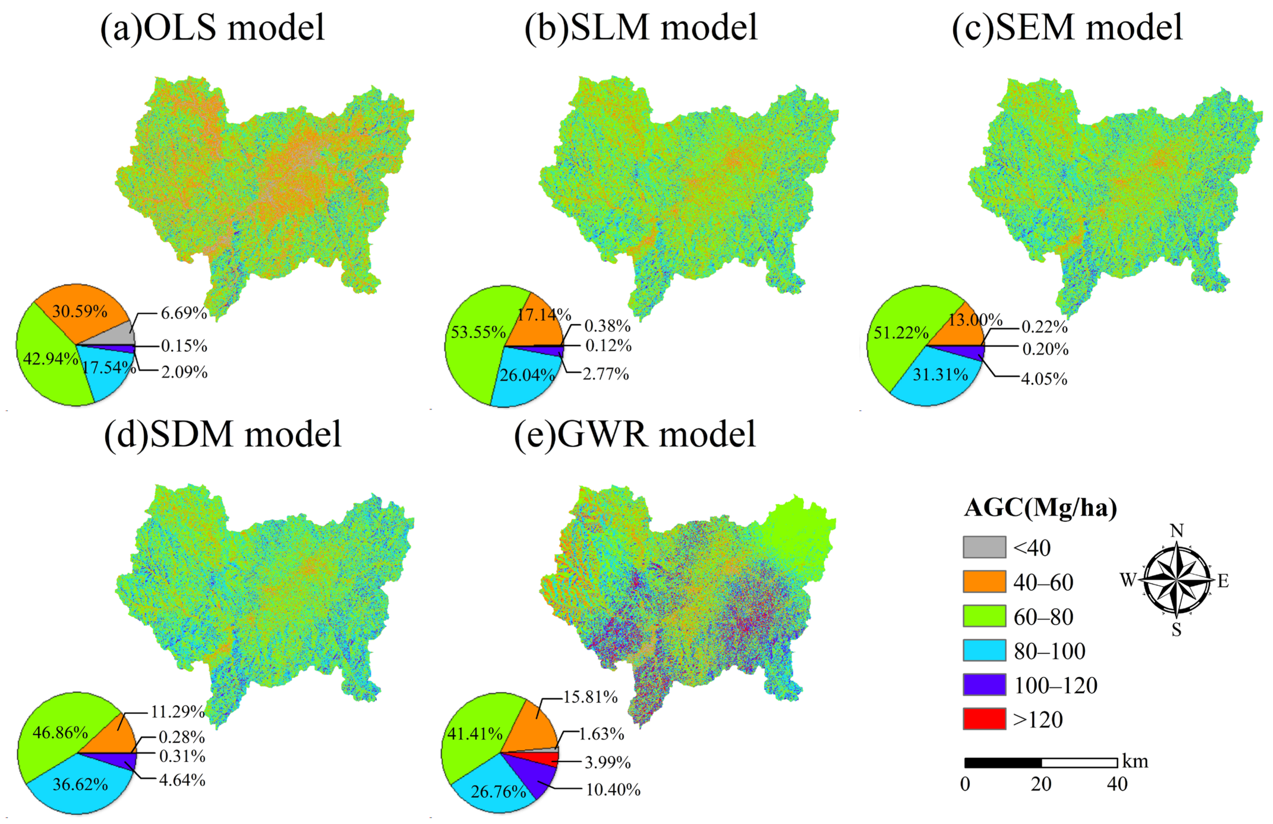
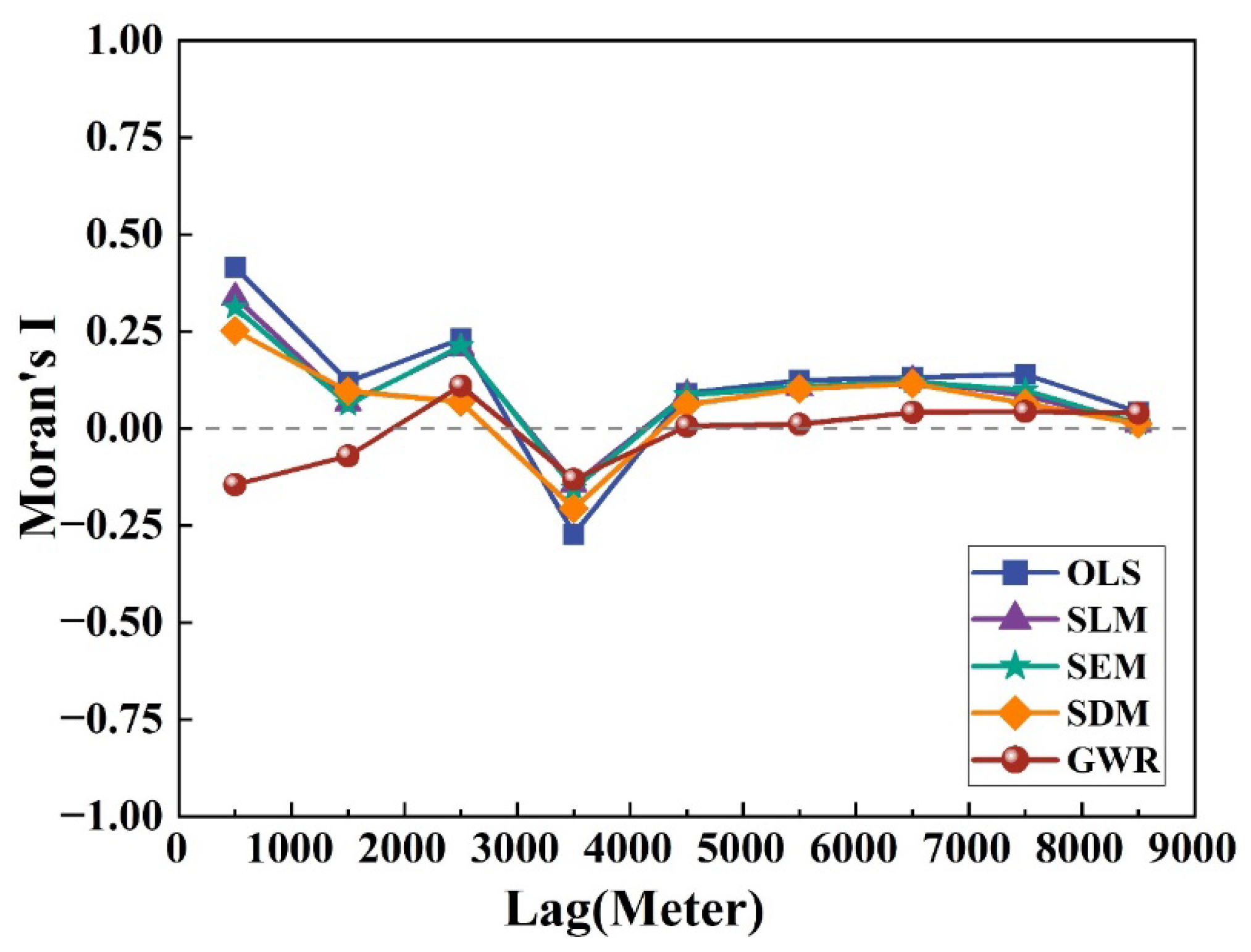
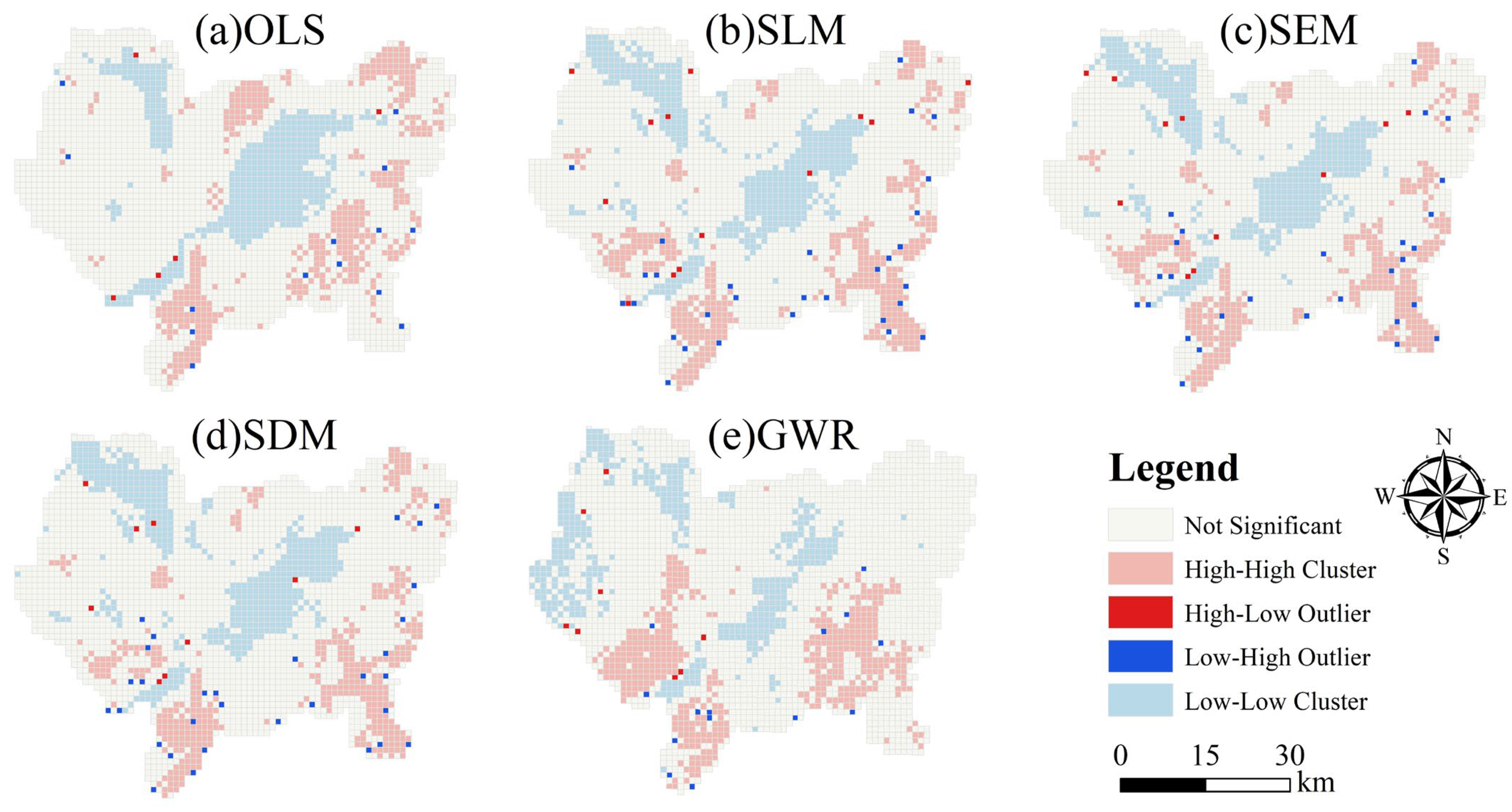
3.4. Spatial Correlation Analysis

The residual Moran’s I of five models for nine different bandwidths in the range of 0 m to 9000 m are compared, as shown in Figure 9. As the bandwidth increases, Moran’s I gradually approaches zero, indicating that the spatial autocorrelation of the model residuals also decreases as the spatial scale increases.

The five models’ residual Moran’s I and the corresponding Z values are listed in

Table 8. Moran’s I and Z score values for the prediction residuals of the five models.

Model	Moran’s I	Z Value
OLS	0.415	2.602
SLM	0.338	1.967
SEM	0.312	1.805
SDM	0.252	1.413
GWR	−0.145	−0.565

. The Z values of OLS and SLM are significantly positive (Z value > 1.96), indicating that these two models are similarly clustered at a significance level of 0.05, while GWR is negative with an absolute value below 1.96. The LISA cluster map provides a clear visualization of the spatial distribution of HH, LL, LH, and HL regions. Figure 10 displays the four significant autocorrelations present within the study area. From the figure, it is evident that the low–low clusters are primarily located in the central region, while the high–high outliers are predominantly situated in the southeastern and southwestern regions. Overall, the GWR has significantly reduced the impact of spatial autocorrelation.

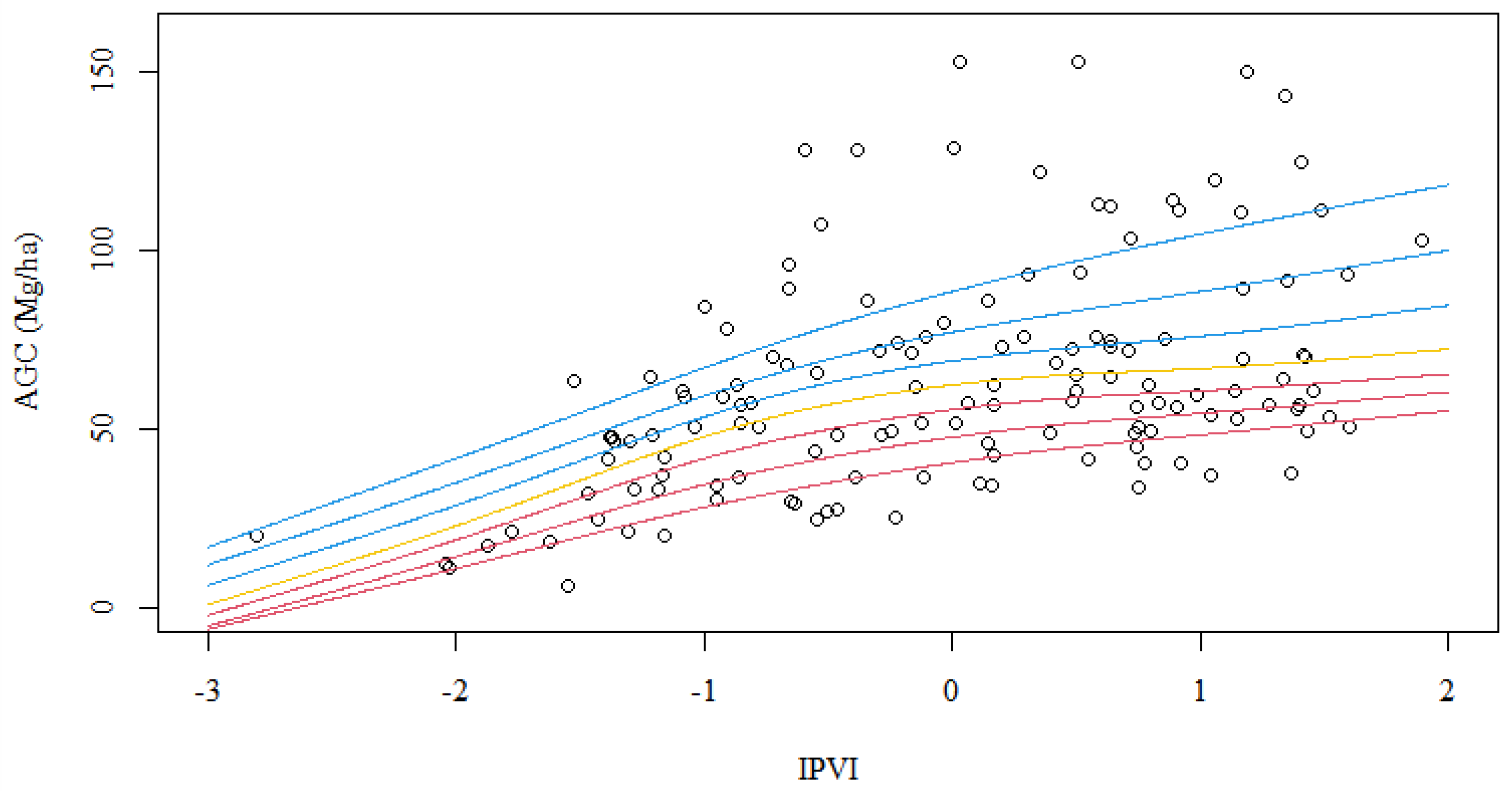
3.5. Determination of Light Saturation Value

Table 9. Estimation results of the AGC light saturation value in Fenglin County.

Variable	Function		${\mathbf{R}}_{\mathbf{adj}}^2$	AIC	Max	DE
IPVI	Linear function		0.198	1312.48	89.608	—
	Quadratic function		0.216	1310.4	76.925	—
	Logarithmic function		0.163	1315.36	91.706	—
	GAM		0.217	1310.15	82.975	22.80%
	QGAM	0.2	0.2	1278.44	54.544	60.80%
		0.3	0.206	1286.69	59.864	44.40%
		0.4	0.208	1292.72	65.058	26.30%
		0.5	0.213	1305.99	71.932	17.10%
		0.6	0.218	1328.18	83.863	15.10%
		0.7	0.213	1345.05	99.007	21.70%
		0.8	0.184	1377.54	117.145	37.60%
All variables	Linear function		0.285	1299.67	100.763	—
	GAM		0.294	1298.8	97.071	31.90%
	QGAM	0.2	0.271	1264.83	65.48	64.70%
		0.3	0.279	1278.12	71.285	52.90%
		0.4	0.274	1284.29	77.862	36.80%
		0.5	0.274	1294.29	85.026	27.40%
		0.6	0.279	1310.25	95.702	23.90%
		0.7	0.285	1331.79	108.832	28.40%
		0.8	0.273	1397.39	129.894	43.50%

shows the fitting estimation results of the AGC light saturation value using the linear regression and nonlinear regression models. The maximum value of the regression results represents the estimated light saturation value of AGC under the respective method. It can be seen that all variables are more interpretable than a single variable, with higher $R_{\mathit{adj}}^2$ and explained deviance and smaller AIC values. Previous studies on optical saturation often relied on a single variable for prediction. This study demonstrates that appropriately additional predictive variables can improve the model’s fitting accuracy, resulting in more realistic and reliable predictions. Although the GAM offers the best fit, it is one-sided to represent the light saturation value of AGC by a single value. The results of fitting all variables to the QGAM can be used as a reference for the range of AGC saturation values.

To further visualize the QGAM, this study shows the QGAM with 138 plot fits applied to the most significant variable IPVI, as shown in Figure 11. In both low-value and high-value regions, the model demonstrates exemplary fitting performance. Relative to a singular linear model, this approach markedly elevates the predictive accuracy, adaptability, and interpretability. At the same time, it allows for segmented evaluation of AGC prediction outcomes from different spatial regression models.

Based on the light saturation value statistics of a single variable and all variables based on QGAM, the proportions of forest AGC area in Fenglin County inverted by each spatial regression model are shown in Figure 12. The figure reveals that the saturation phenomenon is more prominent in the QGAM results based on all variables, and significant differences in estimation among the models are evident within the q range of 0.7–0.8. We consider the results obtained from the QGAM constructed using all variables, within the q value range of 0.7 to 0.8, as the range for AGC light saturation values (108.832 to 129.894 Mg/ha). The global regression model fails to accurately estimate forest AGC within the saturation range and is also incapable of predicting AGC values exceeding this range. The inversion results from the GWR model reveal that the forest AGC in Fenglin County is saturated in approximately 6.26% of the total area and exceeds saturation in about 1.97% of the area. The GWR model to some extent addresses the issue of data saturation when utilizing remote sensing for AGC estimation.

4. Discussion

4.1. Uncertainty Analysis of AGC Estimation

Uncertainties in forest AGC estimation using remote sensing primarily stem from the selection of AGC modeling variables and the choice of algorithm for constructing the AGC estimation model [26]. In this study, a spatial regression model was used to estimate the AGC. From the above model fitting and prediction results, the spatial effect cannot be ignored. Spatial effects can be caused by many factors, such as distance-related species interactions, spatial nonstationarity among variables, and nonlinear relationships between environmental factors and species that are erroneously modeled as linear [81]. Notably, some sample plots in the study area are distributed near villages within the study area, exhibiting lower AGC values. Simultaneously, there is a large spatial heterogeneity among the plots due to the influence of altitude. In this study, GWR was used to explore the spatial distribution of large-scale sample plots. By considering spatial correlation, the AGC spatial heterogeneity is reduced for model construction, which has a strong improvement compared with the OLS model fitting prediction. The GWR model reduces uncertainty in remote sensing estimates by accounting for spatial heterogeneity and correlation, thus mitigating overestimation in high-value areas and underestimation in low-value areas [82]. This finding is consistent with the results obtained by Ou et al., who used Landsat 8 and a spatial regression model for predicting AGB [38]. For AGC estimation methods, there are also nonparametric and machine-learning models, which are higher than GWR in terms of fitting accuracy [30,83]. Li et al. employed Sentinel-2 and used four machine learning methods to estimate forest AGC in Shanghai. They discovered that the model yielding the best predictive results still exhibited instances of overestimation. The researchers attributed this phenomenon to the uneven distribution of samples and the presence of significant spatial heterogeneity within the sample data [30]. Puliti et al. improved the estimation accuracy of AGB in Norway by utilizing ArcticDEM and Sentinel-2 data in conjunction with a random forest model. They indicated that forest characteristics and terrain are sources of uncertainty in model predictions [84]. Although the nonparametric method closely responds to sample data characteristics, its sensitivity is accentuated given the small sample size in this study. In contrast, GWR not only offers superior predictive capabilities but also delivers a more lucid mathematical interpretation. It emphasizes the spatial distribution of the studied multivariate relationship and adeptly accounts for the influences of spatial autocorrelation and heterogeneity on local-scale AGC estimation, making it well suited for analyzing spatial nonstationarity in dynamic environments [85].

4.2. Light Saturation Phenomenon

The issue of light saturation is common when estimating AGC using remote sensing data [10]. In a previous study, Steininger used Landsat data to determine the age and above-ground biomass of 34 tropical secondary forest sites in Manaus, Brazil, and found that data saturation occurred when the above-ground biomass approached approximately 15 kg/m² or when the vegetation reached an age of 15 years or more and canopy reflectance was saturated [86]. Mature forest stands with complex structures can also cause data saturation, and there are many reasons why this may occur [10,87]. Ahmad et al. conducted a study on biomass estimation in moist temperate forests in the Galies region of Abbottabad, Pakistan, using Sentinel-2 remote sensing data. They discovered that the accuracy of Sentinel-2-derived indices was influenced in areas with higher vegetation density [88]. To improve the reliability of above-ground biomass carbon estimation, integrating data from multiple sensors, stratifying AGC estimation based on vegetation types and slope, and combining age virtual variables and texture features have been proposed [26,89]. Visible light saturation is an important factor that results in inaccuracies in estimations of high AGC values. Researchers studying the biomass saturation of temperate forests in China have obtained saturation values that are not significantly different from the results of this study [11]. In this study, the QGAM method was used to accurately estimate the forest AGC light saturation value from 108.832 to 129.894 Mg/ha. It was found that more than 8% of the forest AGC in Fenglin County inverted by the GWR model was in the saturation range, which improved the problem of data saturation compared with the global regression model. This finding indicates that the forest AGC area falling within the light saturation value is not small and the uncertainty caused by data saturation issues cannot be overlooked. Accurately estimating the saturation value of forest AGC is crucial for formulating sensible management strategies and environmental protection policies.

4.3. Limitations and Future Works

This study highlights the benefits of using remote sensing for forest AGC estimation. However, it should be noted that the image quality of optical remote sensing is often compromised by cloud cover. It is recommended to select remote sensing images from spring or summer with cloud cover less than 2% for processing and analysis in order to enhance the usability of the image data. The dataset used in this study is uniformly distributed and representative. The fixed distribution plots measured in the field ensure high data quality. This allows us to not only provide a more comprehensive and accurate analysis of the spatial distribution of forest AGC in Fenglin County but also offer a reference for its precise estimation in the Northeast Forest Region. Additionally, Sentinel-2 data and spatial regression models can also be used for spatial distribution analysis in other fields, such as the spatial variation in crops, soil organic carbon distribution, and air quality [28,46,58]. In the future, it will be essential to analyze the spatial distribution of carbon storage in other forest types and even broader ecosystem contexts. With the implementation of forest conservation policies, it is anticipated that future forest distribution will be dominated by mature forests. It is imperative to delve deeply into the data saturation challenges encountered in remote sensing estimation.

5. Conclusions

Based on Sentinel-2 remote sensing images, we constructed a spatial regression model to predict the spatial distribution of cold temperate forest AGC in Northeast China. This study resulted in the following conclusions: (1) The GWR model constructed by combining vegetation index texture features and terrain factors has the best fitting accuracy and predictive performance. It shows the highest R² (0.695) and the lowest rRMSE (0.273). Following closely were the SDM, SEM, SLM, and OLS models in terms of their performance. (2) The spatial effect should not be ignored, as evidenced by the analysis of model residuals and the spatial distribution inversion of AGC. (3) During AGC estimation using optical remote sensing, a saturation phenomenon occurs. The AGC light saturation values estimated through QGAM range from 108.832 to 129.894 Mg/ha, with a saturated area percentage of 8.23% for forest AGC in Fenglin County.

References

1. Debbarma, J.; Choi, Y. A Taxonomy of Green Governance: A Qualitative and Quantitative Analysis towards Sustainable Development. Sustain. Cities Soc. 2022, 79, 103693. [Google Scholar] [CrossRef]
2. Goosen, M.F.A. Environmental Management and Sustainable Development. Procedia Eng. 2012, 33, 6–13. [Google Scholar] [CrossRef]
3. Pan, Y.; Birdsey, R.A.; Fang, J.; Houghton, R.; Kauppi, P.E.; Kurz, W.A.; Phillips, O.L.; Shvidenko, A.; Lewis, S.L.; Canadell, J.G.; et al. A Large and Persistent Carbon Sink in the World’s Forests. Science 2011, 333, 988–993. [Google Scholar] [CrossRef] [PubMed]
4. Balima, L.H.; Kouamé, F.N.; Bayen, P.; Ganamé, M.; Nacoulma, B.M.I.; Thiombiano, A.; Soro, D. Influence of Climate and Forest Attributes on Aboveground Carbon Storage in Burkina Faso, West Africa. Environ. Chall. 2021, 4, 100123. [Google Scholar] [CrossRef]
5. Bonan, G.B. Forests and Climate Change: Forcings, Feedbacks, and the Climate Benefits of Forests. Science 2008, 320, 1444–1449. [Google Scholar] [CrossRef]
6. Araza, A.; de Bruin, S.; Herold, M.; Quegan, S.; Labriere, N.; Rodriguez-Veiga, P.; Avitabile, V.; Santoro, M.; Mitchard, E.T.A.; Ryan, C.M.; et al. A Comprehensive Framework for Assessing the Accuracy and Uncertainty of Global Above-Ground Biomass Maps. Remote Sens. Environ. 2022, 272, 112917. [Google Scholar] [CrossRef]
7. Vashum, K.T.; Jayakumar, S. Methods to Estimate Above-Ground Biomass and Carbon Stock in Natural Forests—A Review. J. Ecosyst. Ecography 2012, 2, 1–7. [Google Scholar] [CrossRef]
8. Achard, F.; Eva, H.D.; Mayaux, P.; Stibig, H.-J.; Belward, A. Improved Estimates of Net Carbon Emissions from Land Cover Change in the Tropics for the 1990s. Glob. Biogeochem. Cycles 2004, 18, 1–11. [Google Scholar] [CrossRef]
9. Zhu, J.; Hu, H.; Tao, S.; Chi, X.; Li, P.; Jiang, L.; Ji, C.; Zhu, J.; Tang, Z.; Pan, Y.; et al. Carbon Stocks and Changes of Dead Organic Matter in China’s Forests. Nat. Commun. 2017, 8, 151. [Google Scholar] [CrossRef]
10. Lu, D.; Chen, Q.; Wang, G.; Liu, L.; Li, G.; Moran, E. A Survey of Remote Sensing-Based Aboveground Biomass Estimation Methods in Forest Ecosystems. Int. J. Digit. Earth 2016, 9, 63–105. [Google Scholar] [CrossRef]
11. Zhao, P.; Lu, D.; Wang, G.; Wu, C.; Huang, Y.; Yu, S. Examining Spectral Reflectance Saturation in Landsat Imagery and Corresponding Solutions to Improve Forest Aboveground Biomass Estimation. Remote Sens. 2016, 8, 469. [Google Scholar] [CrossRef]
12. Wang, G.; Oyana, T.; Zhang, M.; Adu-Prah, S.; Zeng, S.; Lin, H.; Se, J. Mapping and Spatial Uncertainty Analysis of Forest Vegetation Carbon by Combining National Forest Inventory Data and Satellite Images. For. Ecol. Manag. 2009, 258, 1275–1283. [Google Scholar] [CrossRef]
13. Zhang, G.; Ganguly, S.; Nemani, R.R.; White, M.A.; Milesi, C.; Hashimoto, H.; Wang, W.; Saatchi, S.; Yu, Y.; Myneni, R.B. Estimation of Forest Aboveground Biomass in California Using Canopy Height and Leaf Area Index Estimated from Satellite Data. Remote Sens. Environ. 2014, 151, 44–56. [Google Scholar] [CrossRef]
14. Chen, L.-C.; Guan, X.; Li, H.-M.; Wang, Q.-K.; Zhang, W.-D.; Yang, Q.-P.; Wang, S.-L. Spatiotemporal Patterns of Carbon Storage in Forest Ecosystems in Hunan Province, China. For. Ecol. Manag. 2019, 432, 656–666. [Google Scholar] [CrossRef]
15. Piermattei, L.; Karel, W.; Wang, D.; Wieser, M.; Mokroš, M.; Surový, P.; Koreň, M.; Tomaštík, J.; Pfeifer, N.; Hollaus, M. Terrestrial Structure from Motion Photogrammetry for Deriving Forest Inventory Data. Remote Sens. 2019, 11, 950. [Google Scholar] [CrossRef]
16. Richards, G.P.; Evans, D.M.W. Development of a Carbon Accounting Model (FullCAM Vers. 1.0) for the Australian Continent. Aust. For. 2004, 67, 277–283. [Google Scholar] [CrossRef]
17. Keith, H.; Mackey, B.G.; Lindenmayer, D.B. Re-Evaluation of Forest Biomass Carbon Stocks and Lessons from the World’s Most Carbon-Dense Forests. Proc. Natl. Acad. Sci. USA 2009, 106, 11635–11640. [Google Scholar] [CrossRef]
18. Urbazaev, M.; Thiel, C.; Cremer, F.; Dubayah, R.; Migliavacca, M.; Reichstein, M.; Schmullius, C. Estimation of Forest Aboveground Biomass and Uncertainties by Integration of Field Measurements, Airborne LiDAR, and SAR and Optical Satellite Data in Mexico. Carbon Balance Manag. 2018, 13, 5. [Google Scholar] [CrossRef]
19. Graves, S.J. A Tree-Based Approach to Biomass Estimation from Remote Sensing Data in a Tropical Agricultural Landscape. Remote Sens. Environ. 2018, 218, 32–43. [Google Scholar] [CrossRef]
20. Dube, T.; Mutanga, O. Evaluating the Utility of the Medium-Spatial Resolution Landsat 8 Multispectral Sensor in Quantifying Aboveground Biomass in uMgeni Catchment, South Africa. ISPRS J. Photogramm. Remote Sens. 2015, 101, 36–46. [Google Scholar] [CrossRef]
21. Anand, A.; Pandey, P.C.; Petropoulos, G.P.; Pavlides, A.; Srivastava, P.K.; Sharma, J.K.; Malhi, R.K.M. Use of Hyperion for Mangrove Forest Carbon Stock Assessment in Bhitarkanika Forest Reserve: A Contribution towards Blue Carbon Initiative. Remote Sens. 2020, 12, 597. [Google Scholar] [CrossRef]
22. Sinha, S.; Mohan, S.; Das, A.K.; Sharma, L.K.; Jeganathan, C.; Santra, A.; Santra Mitra, S.; Nathawat, M.S. Multi-Sensor Approach Integrating Optical and Multi-Frequency Synthetic Aperture Radar for Carbon Stock Estimation over a Tropical Deciduous Forest in India. Carbon Manag. 2020, 11, 39–55. [Google Scholar] [CrossRef]
23. Ghasemi, N.; Sahebi, M.; Mohammadzadeh, A. Biomass Estimation of a Temperate Deciduous Forest Using Wavelet Analysis. IEEE Trans. Geosci. Remote Sens. 2013, 51, 765–776. [Google Scholar] [CrossRef]
24. Chen, Q.; Vaglio Laurin, G.; Valentini, R. Uncertainty of Remotely Sensed Aboveground Biomass over an African Tropical Forest: Propagating Errors from Trees to Plots to Pixels. Remote Sens. Environ. 2015, 160, 134–143. [Google Scholar] [CrossRef]
25. Mascaro, J.; Detto, M.; Asner, G.P.; Muller-Landau, H.C. Evaluating Uncertainty in Mapping Forest Carbon with Airborne LiDAR. Remote Sens. Environ. 2011, 115, 3770–3774. [Google Scholar] [CrossRef]
26. Lu, D.; Chen, Q.; Wang, G.; Moran, E.; Batistella, M.; Zhang, M.; Vaglio Laurin, G.; Saah, D. Aboveground Forest Biomass Estimation with Landsat and LiDAR Data and Uncertainty Analysis of the Estimates. Int. J. For. Res. 2012, 2012, 436537. [Google Scholar] [CrossRef]
27. Puliti, S.; Breidenbach, J.; Schumacher, J.; Hauglin, M.; Klingenberg, T.F.; Astrup, R. Above-Ground Biomass Change Estimation Using National Forest Inventory Data with Sentinel-2 and Landsat. Remote Sens. Environ. 2021, 265, 112644. [Google Scholar] [CrossRef]
28. Kamenova, I.; Dimitrov, P. Evaluation of Sentinel-2 Vegetation Indices for Prediction of LAI, fAPAR and fCover of Winter Wheat in Bulgaria. Eur. J. Remote Sens. 2021, 54, 89–108. [Google Scholar] [CrossRef]
29. Hlatshwayo, S.T.; Mutanga, O.; Lottering, R.T.; Kiala, Z.; Ismail, R. Mapping Forest Aboveground Biomass in the Reforested Buffelsdraai Landfill Site Using Texture Combinations Computed from SPOT-6 Pan-Sharpened Imagery. Int. J. Appl. Earth Obs. Geoinf. 2019, 74, 65–77. [Google Scholar] [CrossRef]
30. Li, H.; Zhang, G.; Zhong, Q.; Xing, L.; Du, H. Prediction of Urban Forest Aboveground Carbon Using Machine Learning Based on Landsat 8 and Sentinel-2: A Case Study of Shanghai, China. Remote Sens. 2023, 15, 284. [Google Scholar] [CrossRef]
31. Zhu, Y.; Liu, K.; Myint, S.W.; Du, Z.; Li, Y.; Cao, J.; Liu, L.; Wu, Z. Integration of GF2 Optical, GF3 SAR, and UAV Data for Estimating Aboveground Biomass of China’s Largest Artificially Planted Mangroves. Remote Sens. 2020, 12, 2039. [Google Scholar] [CrossRef]
32. Labrecque, S.; Fournier, R.A.; Luther, J.E.; Piercey, D. A Comparison of Four Methods to Map Biomass from Landsat-TM and Inventory Data in Western Newfoundland. For. Ecol. Manag. 2006, 226, 129–144. [Google Scholar] [CrossRef]
33. Roy, D.P.; Wulder, M.A.; Loveland, T.R.; Woodcock, C.E.; Allen, R.G.; Anderson, M.C.; Helder, D.; Irons, J.R.; Johnson, D.M.; Kennedy, R.; et al. Landsat-8: Science and Product Vision for Terrestrial Global Change Research. Remote Sens. Environ. 2014, 145, 154–172. [Google Scholar] [CrossRef]
34. Li, Y.; Han, N.; Li, X.; Du, H.; Mao, F.; Cui, L.; Liu, T.; Xing, L. Spatiotemporal Estimation of Bamboo Forest Aboveground Carbon Storage Based on Landsat Data in Zhejiang, China. Remote Sens. 2018, 10, 898. [Google Scholar] [CrossRef]
35. Duysak, H.; Yïğït, E. Investigation of the Performance of Different Wavelet-Based Fusions of SAR and Optical Images Using Sentinel-1 and Sentinel-2 Datasets. Int. J. Eng. Geosci. 2022, 7, 81–90. [Google Scholar] [CrossRef]
36. Chen, Q.; McRoberts, R.E.; Wang, C.; Radtke, P.J. Forest Aboveground Biomass Mapping and Estimation across Multiple Spatial Scales Using Model-Based Inference. Remote Sens. Environ. 2016, 184, 350–360. [Google Scholar] [CrossRef]
37. McEwan, R.W.; Lin, Y.-C.; Sun, I.-F.; Hsieh, C.-F.; Su, S.-H.; Chang, L.-W.; Song, G.-Z.M.; Wang, H.-H.; Hwong, J.-L.; Lin, K.-C.; et al. Topographic and Biotic Regulation of Aboveground Carbon Storage in Subtropical Broad-Leaved Forests of Taiwan. For. Ecol. Manag. 2011, 262, 1817–1825. [Google Scholar] [CrossRef]
38. Ou, G.; Lv, Y.; Xu, H.; Wang, G. Improving Forest Aboveground Biomass Estimation of Pinus Densata Forest in Yunnan of Southwest China by Spatial Regression Using Landsat 8 Images. Remote Sens. 2019, 11, 2750. [Google Scholar] [CrossRef]
39. Yue, T.X.; Wang, Y.F.; Du, Z.P.; Zhao, M.W.; Zhang, L.L.; Zhao, N.; Lu, M.; Larocque, G.R.; Wilson, J.P. Analysing the Uncertainty of Estimating Forest Carbon Stocks in China. Biogeosciences 2016, 13, 3991–4004. [Google Scholar] [CrossRef]
40. Du, H.; Zhou, G.; Fan, W.; Ge, H.; Xu, X.; Shi, Y.; Fan, W. Spatial Heterogeneity and Carbon Contribution of Aboveground Biomass of Moso Bamboo by Using Geostatistical Theory. Plant Ecol. 2010, 207, 131–139. [Google Scholar] [CrossRef]
41. Fox, J.C.; Bi, H.; Ades, P.K. Spatial Dependence and Individual-Tree Growth Models. For. Ecol. Manag. 2007, 245, 10–19. [Google Scholar] [CrossRef]
42. Kint, V.; van Meirvenne, M.; Nachtergale, L.; Geudens, G.; Lust, N. Spatial Methods for Quantifying Forest Stand Structure Development: A Comparison Between Nearest-Neighbor Indices and Variogram Analysis. For. Sci. 2003, 49, 36–49. [Google Scholar] [CrossRef]
43. Zhang, L.; Ma, Z.; Guo, L. An Evaluation of Spatial Autocorrelation and Heterogeneity in the Residuals of Six Regression Models. For. Sci. 2009, 55, 533–548. [Google Scholar]
44. Zhang, L.; Shi, H. Local Modeling of Tree Growth by Geographically Weighted Regression. For. Sci. 2004, 50, 225–244. [Google Scholar] [CrossRef]
45. Shi, W.; Hou, J.; Shen, X.; Xiang, R. Exploring the Spatio-Temporal Characteristics of Urban Thermal Environment during Hot Summer Days: A Case Study of Wuhan, China. Remote Sens. 2022, 14, 6084. [Google Scholar] [CrossRef]
46. Fang, C.; Liu, H.; Li, G.; Sun, D.; Miao, Z. Estimating the Impact of Urbanization on Air Quality in China Using Spatial Regression Models. Sustainability 2015, 7, 15570–15592. [Google Scholar] [CrossRef]
47. Kupfer, J.A.; Farris, C.A. Incorporating Spatial Non-Stationarity of Regression Coefficients into Predictive Vegetation Models. Landsc. Ecol 2007, 22, 837–852. [Google Scholar] [CrossRef]
48. Foody, G.M. Geographical Weighting as a Further Refinement to Regression Modelling: An Example Focused on the NDVI–Rainfall Relationship. Remote Sens. Environ. 2003, 88, 283–293. [Google Scholar] [CrossRef]
49. Luo, K. Spatial Pattern of Forest Carbon Storage in the Vertical and Horizontal Directions Based on HJ-CCD Remote Sensing Imagery. Remote Sens. 2019, 11, 788. [Google Scholar] [CrossRef]
50. Ren, Y.; Lü, Y.; Fu, B.; Comber, A.; Li, T.; Hu, J. Driving Factors of Land Change in China’s Loess Plateau: Quantification Using Geographically Weighted Regression and Management Implications. Remote Sens. 2020, 12, 453. [Google Scholar] [CrossRef]
51. Nie, T.; Zhang, Z.; Qi, Z.; Chen, P.; Sun, Z.; Liu, X. Characterizing Spatiotemporal Dynamics of CH4 Fluxes from Rice Paddies of Cold Region in Heilongjiang Province under Climate Change. Int. J. Environ. Res. Public Health 2019, 16, 692. [Google Scholar] [CrossRef] [PubMed]
52. Yang, G.T.; Li, F.R.; Yin, T.; Jia, W.W.; Li, F.; Jin, X.J. Forest Carbon Storage Distribution and Dynamics in Heilongjiang Province, 1st ed.; Wang, C.Y., Ed.; Northeast Forestry University Press: Harbin, China, 2017; Volume 1, pp. 8–57. ISBN 978-7-5674-1007-7. [Google Scholar]
53. Drusch, M.; Del Bello, U.; Carlier, S.; Colin, O.; Fernandez, V.; Gascon, F.; Hoersch, B.; Isola, C.; Laberinti, P.; Martimort, P.; et al. Sentinel-2: ESA’s Optical High-Resolution Mission for GMES Operational Services. Remote Sens. Environ. 2012, 120, 25–36. [Google Scholar] [CrossRef]
54. Sun, H.; Wang, Q.; Wang, G.; Lin, H.; Luo, P.; Li, J.; Zeng, S.; Xu, X.; Ren, L. Optimizing kNN for Mapping Vegetation Cover of Arid and Semi-Arid Areas Using Landsat Images. Remote Sens. 2018, 10, 1248. [Google Scholar] [CrossRef]
55. Becker, F.; Choudhury, B.J. Relative Sensitivity of Normalized Difference Vegetation Index (NDVI) and Microwave Polarization Difference Index (MPDI) for Vegetation and Desertification Monitoring. Remote Sens. Environ. 1988, 24, 297–311. [Google Scholar] [CrossRef]
56. Jordan, C.F. Derivation of Leaf-Area Index from Quality of Light on the Forest Floor. Ecology 1969, 50, 663–666. [Google Scholar] [CrossRef]
57. Fatiha, B.; Abdelkader, A.; Latifa, H.; Mohamed, E. Spatio Temporal Analysis of Vegetation by Vegetation Indices from Multi-Dates Satellite Images: Application to a Semi Arid Area in ALGERIA. Energy Procedia 2013, 36, 667–675. [Google Scholar] [CrossRef]
58. Gholizadeh, A.; Žižala, D.; Saberioon, M.; Borůvka, L. Soil Organic Carbon and Texture Retrieving and Mapping Using Proximal, Airborne and Sentinel-2 Spectral Imaging. Remote Sens. Environ. 2018, 218, 89–103. [Google Scholar] [CrossRef]
59. Haralick, R.M.; Shanmugam, K.; Dinstein, I. Textural Features for Image Classification. IEEE Trans. Syst. Man Cybern. 1973, 6, 610–621. [Google Scholar] [CrossRef]
60. Luo, S.; Wang, C.; Xi, X.; Pan, F.; Qian, M.; Peng, D.; Nie, S.; Qin, H.; Lin, Y. Retrieving Aboveground Biomass of Wetland Phragmites Australis (Common Reed) Using a Combination of Airborne Discrete-Return LiDAR and Hyperspectral Data. Int. J. Appl. Earth Obs. Geoinf. 2017, 58, 107–117. [Google Scholar] [CrossRef]
61. Qasim, M.; Mahmood, D.; Bibi, A.; Masud, M.; Ahmed, G.; Khan, S.; Jhanjhi, N.Z.; Hussain, S.J. PCA-Based Advanced Local Octa-Directional Pattern (ALODP-PCA): A Texture Feature Descriptor for Image Retrieval. Electronics 2022, 11, 202. [Google Scholar] [CrossRef]
62. Menke, W. Review of the Generalized Least Squares Method. Surv. Geophys. 2015, 36, 1–25. [Google Scholar] [CrossRef]
63. Lee, L.-F.; Yu, J. Near Unit Root in the Spatial Autoregressive Model. Spat. Econ. Anal. 2013, 8, 314–351. [Google Scholar] [CrossRef]
64. LeSage, J.P. Bayesian Estimation of Limited Dependent Variable Spatial Autoregressive Models. Geogr. Anal. 2010, 32, 19–35. [Google Scholar] [CrossRef]
65. Anselin, L. Spatial Econometrics: Methods and Models; Springer Science & Business Media: Berlin/Heidelberg, Germany, 1988; ISBN 978-90-247-3735-2. [Google Scholar]
66. Mur, J.; Angulo, A. The Spatial Durbin Model and the Common Factor Tests. Spat. Econ. Anal. 2006, 1, 207–226. [Google Scholar] [CrossRef]
67. Brunsdon, C.; Fotheringham, A.S.; Charlton, M.E. Geographically Weighted Regression: A Method for Exploring Spatial Nonstationarity. Geogr. Anal. 2010, 28, 281–298. [Google Scholar] [CrossRef]
68. Sun, Y.; Ao, Z.; Jia, W.; Chen, Y.; Xu, K. A Geographically Weighted Deep Neural Network Model for Research on the Spatial Distribution of the down Dead Wood Volume in Liangshui National Nature Reserve (China). iForest 2021, 14, 353–361. [Google Scholar] [CrossRef]
69. Tutmez, B.; Kaymak, U.; Tercan, A.E. Local Spatial Regression Models: A Comparative Analysis on Soil Contamination. Stoch. Environ. Res. Risk Assess. 2012, 26, 1013–1023. [Google Scholar] [CrossRef]
70. Nabipour, N.; Daneshfar, R.; Rezvanjou, O.; Mohammadi-Khanaposhtani, M.; Baghban, A.; Xiong, Q.; Li, L.K.B.; Habibzadeh, S.; Doranehgard, M.H. Estimating Biofuel Density via a Soft Computing Approach Based on Intermolecular Interactions. Renew. Energy 2020, 152, 1086–1098. [Google Scholar] [CrossRef]
71. Hayes, A.F.; Matthes, J. Computational Procedures for Probing Interactions in OLS and Logistic Regression: SPSS and SAS Implementations. Behav. Res. Methods 2009, 41, 924–936. [Google Scholar] [CrossRef]
72. Anselin, L.; Kelejian, H.H. Testing for Spatial Error Autocorrelation in the Presence of Endogenous Regressors. Int. Reg. Sci. Rev. 1997, 20, 153–182. [Google Scholar] [CrossRef]
73. Anselin, L. Spatial Econometrics. In A Companion to Theoretical Econometrics; Baltagi, B.H., Ed.; Blackwell Publishing Ltd.: Malden, MA, USA, 2003; pp. 310–330. ISBN 978-0-470-99624-9. [Google Scholar]
74. Yang, L.; Yu, K.; Ai, J.; Liu, Y.; Yang, W.; Liu, J. Dominant Factors and Spatial Heterogeneity of Land Surface Temperatures in Urban Areas: A Case Study in Fuzhou, China. Remote Sens. 2022, 14, 1266. [Google Scholar] [CrossRef]
75. Wei, Q.; Zhang, L.; Duan, W.; Zhen, Z. Global and Geographically and Temporally Weighted Regression Models for Modeling PM2.5 in Heilongjiang, China from 2015 to 2018. Int. J. Environ. Res. Public Health 2019, 16, 5107. [Google Scholar] [CrossRef] [PubMed]
76. Zhang, F.; Yushanjiang, A.; Jing, Y. Assessing and Predicting Changes of the Ecosystem Service Values Based on Land Use/Cover Change in Ebinur Lake Wetland National Nature Reserve, Xinjiang, China. Sci. Total Environ. 2019, 656, 1133–1144. [Google Scholar] [CrossRef] [PubMed]
77. Gomez-Rubio, V. Generalized Additive Models: An Introduction with R (2nd Edition). J. Stat. Soft. 2018, 86, 1–5. [Google Scholar] [CrossRef]
78. Fasiolo, M.; Wood, S.N.; Zaffran, M.; Nedellec, R.; Goude, Y. Qgam: Bayesian Nonparametric Quantile Regression Modeling in R. J. Stat. Soft. 2021, 100, 1–31. [Google Scholar] [CrossRef]
79. Miller, H.J. Geographic Representation in Spatial Analysis. J. Geogr. Syst. 2000, 2, 55–60. [Google Scholar] [CrossRef]
80. Ord, J.K.; Getis, A. Local Spatial Autocorrelation Statistics: Distributional Issues and an Application. Geogr. Anal. 2010, 27, 286–306. [Google Scholar] [CrossRef]
81. Dormann, C.F.; McPherson, J.M.; Araújo, M.B.; Bivand, R.; Bolliger, J.; Carl, G.; Davies, R.G.; Hirzel, A.; Jetz, W.; Kissling, W.D.; et al. Methods to Account for Spatial Autocorrelation in the Analysis of Species Distributional Data: A Review. Ecography 2007, 30, 609–628. [Google Scholar] [CrossRef]
82. Fotheringham, A.S.; Charlton, M.E.; Brunsdon, C. Geographically Weighted Regression: A Natural Evolution of the Expansion Method for Spatial Data Analysis. Environ. Plan. A 1998, 30, 1905–1927. [Google Scholar] [CrossRef]
83. Behrens, T.; Schmidt, K.; Viscarra Rossel, R.A.; Gries, P.; Scholten, T.; MacMillan, R.A. Spatial Modelling with Euclidean Distance Fields and Machine Learning. Eur. J. Soil Sci. 2018, 69, 757–770. [Google Scholar] [CrossRef]
84. Puliti, S.; Hauglin, M.; Breidenbach, J.; Montesano, P.; Neigh, C.S.R.; Rahlf, J.; Solberg, S.; Klingenberg, T.F.; Astrup, R. Modelling Above-Ground Biomass Stock over Norway Using National Forest Inventory Data with ArcticDEM and Sentinel-2 Data. Remote Sens. Environ. 2020, 236, 111501. [Google Scholar] [CrossRef]
85. Sun, Y.; Jia, W.; Zhu, W.; Zhang, X.; Saidahemaiti, S.; Hu, T.; Guo, H. Local Neural-Network-Weighted Models for Occurrence and Number of down Wood in Natural Forest Ecosystem. Sci. Rep. 2022, 12, 6375. [Google Scholar] [CrossRef] [PubMed]
86. Steininger, M.K. Satellite Estimation of Tropical Secondary Forest Above-Ground Biomass: Data from Brazil and Bolivia. Int. J. Remote Sens. 2000, 21, 1139–1157. [Google Scholar] [CrossRef]
87. Lu, D.; Batistella, M.; Moran, E. Satellite Estimation of Aboveground Biomass and Impacts of Forest Stand Structure. Photogramm. Eng. Remote Sens. 2005, 71, 967–974. [Google Scholar] [CrossRef]
88. Ahmad, N.; Ullah, S.; Zhao, N.; Mumtaz, F.; Ali, A.; Ali, A.; Tariq, A.; Kareem, M.; Imran, A.B.; Khan, I.A.; et al. Comparative Analysis of Remote Sensing and Geo-Statistical Techniques to Quantify Forest Biomass. Forests 2023, 14, 379. [Google Scholar] [CrossRef]
89. Ou, G.; Li, C.; Lv, Y.; Wei, A.; Xiong, H.; Xu, H.; Wang, G. Improving Aboveground Biomass Estimation of Pinus Densata Forests in Yunnan Using Landsat 8 Imagery by Incorporating Age Dummy Variable and Method Comparison. Remote Sens. 2019, 11, 738. [Google Scholar] [CrossRef]
Figure 1. (a) The figure shows the location of the study area in Fenglin County, Heilongjiang Province, China, and the distribution of the digital elevation model (DEM) across Heilongjiang Province. (b) The figure shows the Sentinel-2 image of Fenglin County and the distribution of 138 plots in the study area in 2021.
Forests 14 01970 g001
Figure 2. Sample plot photos. Figures (ad) depict the site conditions of the actual study plots, with figures (b,c) specifically showing the standard plot corner stakes and the use of a compass clinometer for establishing the survey plot.
Forests 14 01970 g002
Figure 3. Flowchart of steps used in our study. The research is divided into several parts, including basic data processing, model fitting, determination of light saturation value, AGC spatial distribution inversion, and statistical analysis.
Forests 14 01970 g003
Figure 4. Correlation analysis of AGC and remote sensing factors. The value range of the Pearson correlation coefficient is between −1 and 1, red (p > 0) represents a positive correlation, and blue (p < 0) represents a negative correlation. The smaller and darker the ellipse is, the higher the correlation between the two variables. The green box represents the correlation between the dependent variable AGC and each independent variable. The correlation coefficients are listed in the bottom-left corner of the table. The variables selected as the final choices for stepwise regression are surrounded by red boxes: 5, 39, 55, and 56.
Forests 14 01970 g004
Figure 5. Variation trend of different variables and actual above-ground carbon reserves along longitude and latitude. The X-axis represents longitude, the Y-axis represents latitude, and the Z-axis represents the values of different variables. Figures (ae) illustrate the spatial distribution of variables IPVI, B3EN, SLOPE, Aspect, and AGC, showing their respective values at different locations.
Forests 14 01970 g005
Figure 6. Local spatial autocorrelation. The red points represent high–high clusters; the yellow points represent high–low outliers; the green points represent low–high outliers; the blue points represent low–low clusters; and the black points represent nonsignificant local spatial autocorrelation.
Forests 14 01970 g006
Figure 7. The relationship between observed and predicted AGC (Mg/ha) for 103 plots using the ordinary least squares model (OLS) and 4 spatial regression models (SLM, SEM, SDM, and GWR). The blue points represent the sample data, the dashed line represents the central line, and the red line represents the fitted line. The closer the red line is to the central line, the better the model fit is.
Forests 14 01970 g007
Figure 8. Spatial distribution of forest AGC in Fenglin County by five models in 2021: (a) OLS, (b) SLM, (c) SEM, (d) SDM, and (e) GWR model. The pie chart shows the proportion of carbon storage area distribution in each interval.
Forests 14 01970 g008
Figure 9. Moran’s I of the model residual under different bandwidths.
Forests 14 01970 g009
Figure 10. LISA cluster map of the five models.
Forests 14 01970 g010
Figure 11. The QGAM fitted by the most significant variable IPVI (after standardization) (note: the red line is the QGAM of q = 0.2, 0.3, 0.4 from bottom to top; the yellow line is the QGAM of q = 0.5; the blue line is from bottom to top QGAM with q = 0.6, 0.7, 0.8, respectively). The white circle is the AGC data of the measured sample plot.
Forests 14 01970 g011
Figure 12. Based on the light saturation value results of QGAM’s single variable and all variables, the statistics of the proportion of forest AGC area in Fenglin County across each spatial regression model’s inversions.
Forests 14 01970 g012