Interacting Sentinel-2A, Sentinel 1A, and GF-2 Imagery to Improve the Accuracy of Forest Aboveground Biomass Estimation in a Dry-Hot Valley

Abstract

Carbon absorption and storage in forests is one of the important ways to mitigate climate change. Therefore, it is essential to use a variety of remote-sensing resources to accurately estimate forest aboveground biomass (AGB) in dry-hot valley regions. In this study, satellite images from the Sentinel-1A, Sentinel-2A, and Gaofen-2 satellites were utilized to estimate the forest AGB in Yuanmou County, Yunnan Province, China. Different combinations of image data, based on selected variables of stepwise regression and their performance in constructing linear stepwise regression (LSR) and random forest (RF) models, were explored. The results showed that: (1) after adding the polarized values of the synthetic aperture radar backscatter coefficients, the combination fitting effect was significantly improved; (2) the fitting effect of the Sentinel-1A + Sentinel-2A + Gaofen-2 data combination was superior to the other combinations, indicating that the effective extraction of forest horizon and vertical information can improve the estimation effect of the forest AGB; and (3) the RF model exhibited superior fitting performance compared to the LSR model across all permutations of remotely sensed image datasets, with R² values of 0.71 and 0.65, and RMSE values of 30.67 and 33.79 Mg/ha, respectively. These findings lay the groundwork for enhancing the precision of AGB estimation in dry-hot valley areas by integrating Sentinel-2A, Sentinel-1A, and GF-2 imagery, providing valuable insights for future research and applications.

1. Introduction

Forest above-ground biomass (AGB) plays a fundamental and indispensable role in the global carbon cycle and contributes to the mitigation of global climate change [1,2,3]. Hence, it is important to be able to estimate the forest AGB accurately and rapidly. However, traditional methods of biomass estimation in the field are destructive, time-consuming, and spatially limited, although the results tend to be accurate [4]. However, the remote-sensing assessment of AGB has the advantages of remote-sensing technology, with its multi-temporal, multi-scale, multi-sensor, and rapid monitoring, which can easily overcome the limitations of traditional AGB survey methods [5,6,7]. Therefore, using remote-sensing technology to achieve high-precision estimates of forest AGB has become a hot research topic [8].

Due to the excellent characteristics of different remote-sensing datasets, they are widely used in the fields of forestry, snow cover, agriculture, medicine, oceans, regression, and others [9,10,11]. By estimating forest AGB, we can help manage and protect our forest resources more effectively, as well as cope with today’s growing challenges of climate change. Studies have utilized various remote sensing datasets to improve the precision of AGB estimation, spanning from local to global scales [7]. Santoro et al. [12] combined multiple synthetic-aperture radar (SAR) satellite observations from around 2010 to generate a global aboveground living biomass dataset that could have a significant impact on climate, carbon, and socioeconomic modeling, and provide a basis for future estimates of carbon stock changes. Among these, multispectral remote-sensing data possess the benefits of being both multi-temporal and multi-resolution, providing rich spectral information, with advanced technology utilizing infrared bands sensitive to plant data, this method has been extensively employed in estimating forest biomass [13,14]. The Sentinel-2A (S2) satellites are open-source, with rich band information, moderate spatial and temporal resolution, and a wide detection range. The S2 possesses a 10-m spatial resolution along with 13 bands, and its unique three “vegetation red edge” bands can provide more data support for the monitoring of surface planting [15,16]. In addition, the high spatial resolution multi-spectral images from the Gaofen-2 (GF-2) satellite can represent vegetation information well and have been gradually utilized in remotely sensed biomass estimation studies [17,18,19]. The GF-2 has a high spatial resolution and can realize a more-detailed extraction of forest feature information and provide more-detailed spatial information, which is suitable for small-scale vegetation biomass monitoring and change analysis. These data sources have found extensive application in remote-sensing estimations of forest AGB [20,21,22]. However, researchers have found that optical sensor data suffers from homonyms and homographs, and that saturation is another major issue contributing to the poor performance of AGB estimation, especially in forest stands in areas of high heterogeneity [23]. In response, SAR benefits from its capability to penetrate through the forest canopy, enabling the acquisition of trunk-related information, is not affected by the weather, is able to operate under all weather conditions and holds significant promise for estimating forest AGB [24,25,26]. In addition, SAR can improve the saturation value of optical remote sensing to some extent. Sentinel-1A (S1) images can obtain forest vertical information. Because of the interaction between the microwave signal and the forest, forest structure information can be obtained, which is helpful to the study of forest biomass [27]. Although different degrees of success have been achieved in forest AGB remote-sensing estimation based on GF-2, S2, and S1 images, there are still limitations to obtaining forest biomass information based on single images [28,29]. By combining multi-spectral data with SAR data for AGB estimation, the fitting performance can be effectively improved. Multiple investigations have demonstrated that integrating various remote-sensing techniques can mitigate the limitations of individual sensors. This integration offers complementary benefits that can enhance the precision of forest AGB estimation [30,31,32]. For example, Forkuora et al. [33] utilized S1 and S2 for remotely estimating the AGB in dryland forests and found that combining these data with SAR data could improve the estimates. Zhu et al. [34] combined multi-source datasets (GF-2, GF-3 SAR, and a digital surface model [DSM]) to estimate the AGB of mangrove forests, thereby producing higher estimation accuracy. Regarding spatial resolution, spectral variability, and obtaining the vertical structure of forest stands, GF-2, S2, and SAR images are superior. However, there is a scarcity of research that has delved into the efficacy of using a combination of three images concurrently––GF-2, S1, and S2––in estimating forest AGB. Hence, we integrated three types of image features with the aim of improving the precision of the AGB estimation.

Model choice and effectiveness are key to accurately estimating forest biomass via remote-sensing data [6,35]. Hence, selecting an appropriate model is of the utmost importance. Parametric and non-parametric algorithms have commonly been employed in AGB estimation [36]. Parametric models perform well on small datasets, have an intuitive understanding of the relationships between variables, and are easy to interpret. The parametric model employs various functions, including linear, power, and exponential, to establish correlations among AGB and independent variables. The linear stepwise regression (LSR) algorithm employs significance tests to discern crucial variables in modeling, thus improving the estimation accuracy of the parametric model to some degree. Therefore, it has become a common biomass modeling algorithm [7]. Moreover, machine-learning algorithms exhibit greater flexibility, robustness, and generalization capabilities when handling large-scale datasets. These algorithms can effectively capture the intricate nonlinear relationship between variables of remote-sensing data and forest AGB. This leads to a significant enhancement in accuracy, providing more reliable estimates for forest AGB [37]. Random forest (RF), for instance, is widely applied in AGB remote-sensing estimation due to its adjustability, robustness, high precision, and fast efficiency [38,39].

The dry-hot valley of the Jinsha River is located in Southwestern China. It is an ecologically fragile area known for its sparse vegetation cover, high evapotranspiration, and severe soil erosion [40]. It has the unique savanna vegetation of a dry-hot valley, characterized by sparse trees, shrubs, and herbs along the slopes [41]. After an extensive literature review, few estimates of the AGB in dry-hot valley forests were found. There has been no comprehensive study on the AGB of dry-hot valley forests using the three kinds of multi-source remote sensing described above. Therefore, the objectives aimed for in this study were: (1) to explore the fitting performance of different image combinations (S1 + S2, S1 + GF-2, S2 + GF-2, S1 + S2 + GF-2) in forest AGB estimation in a dry-hot valley; and (2) to compare the fitting effect of the LSR and RF under the various image combinations.

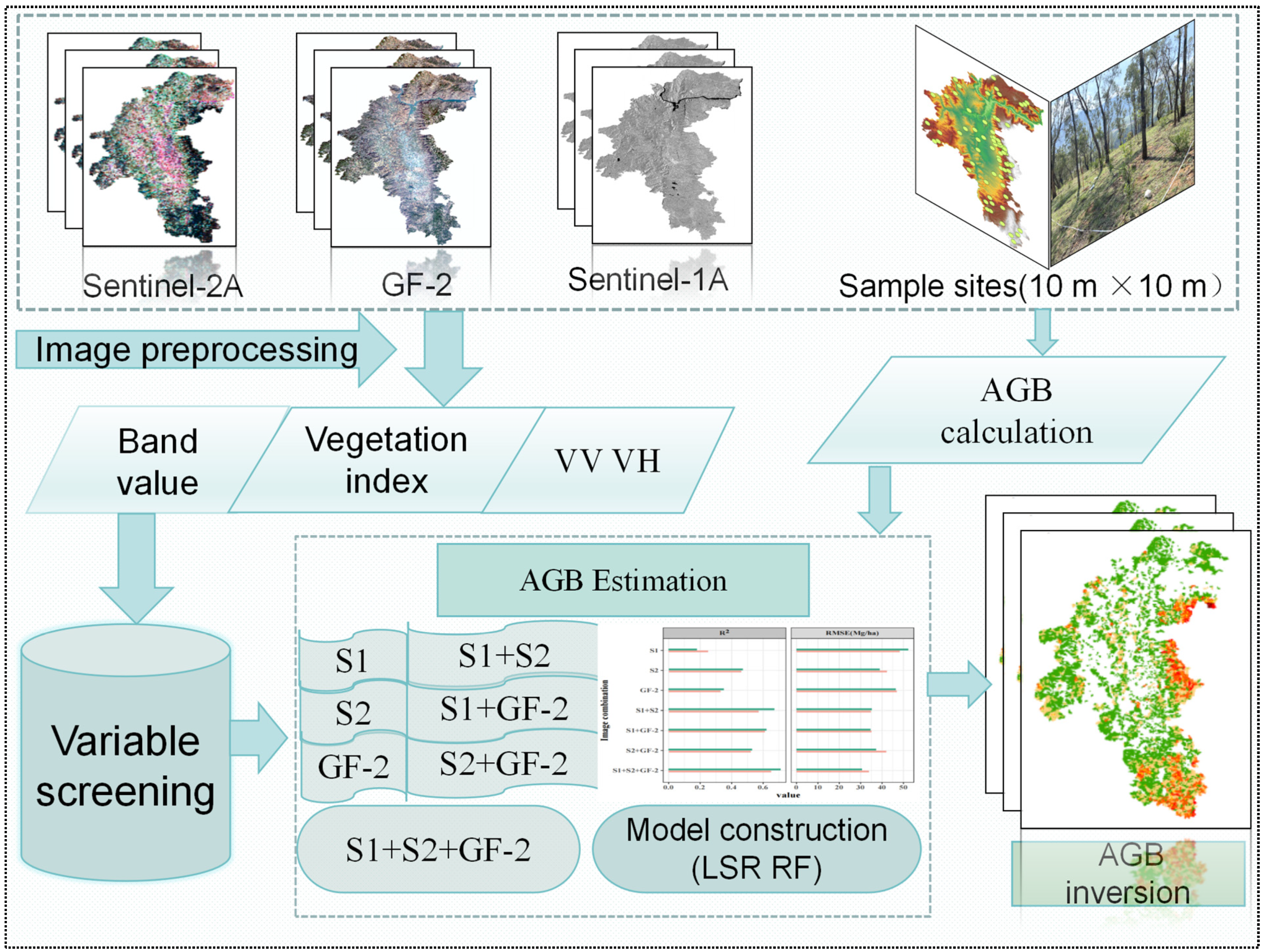
2. Material and Methods

The research process flowchart is illustrated in Figure 1. This study involved: (1) collecting GF-2, S1, and S2 remote-sensing images along with field sample plot data; (2) extracting remote-sensing data by pre-processing and correlation; (3) selecting the stepwise regression variable; (4) combining the datasets of the remote-sensing factors from the different data sources; (5) constructing models and performing evaluations; and (6) forecasting and cartographically representing the spatial distribution of within the research region.

2.1. Study Area

The study area spanned an administrative area of approximately 2020 km² in Yuanmou County in Yunnan Province, China. The study area stretches 50 km from east to west. Additionally, it extends 85 km from north to south. Its geographical location lies between 101°35′–102°6′ E and 25°23′–26°6′ N (Figure 2) [41]. Here, the Jinsha River runs through a typical dry-hot valley, the lowest elevation of which is 898 m and the highest is 2836 m. The area experiences clear distinctions between dry and wet seasons, with an average yearly temperature recorded at 21.9 °C and the highest temperature reaching above 40 °C. The region experiences a mean yearly evaporation of 3847.8 mm, significantly surpassing the mean yearly rainfall of just 634 mm. Thus, the average annual evaporation is much greater than the annual precipitation [42]. The zonal vegetation in the Jinsha River dry-hot valley includes subtropical semi-humid evergreen broad-leaved forests and coniferous forests. There are large areas covered with shrubs and grasslands, while smaller areas are planted with eucalyptus trees.

2.2. Materials

2.2.1. Field Data Collection and Biomass Calculation

Data were collected from the plots based on the distribution of tree species and geographical characteristics in August 2022, the data were gathered from trees with a diameter at breast height (DBH) exceeding 5 cm. There were 78 plots (10 m × 10 m) in total dedicated to the tree survey. Each plot’s centroid coordinates were documented using real-time kinematic positioning, following the World Geodetic System 84 standard [43]. The tree survey mainly included information on the tree species, tree height, DBH, and crown width. The arrangement of the sampling sites is depicted in Figure 2. The plots were selected to cover the primary distribution areas of tree species in Yuanmou County. The tree species recorded included Pinus yunnanensis Franch., Eucalyptus L’Hér, Quercus franchetii Skan., Pinus armandii Franch., Keteleeria fortunei (A. Murray bis) Carrière., Phyllanthus emblica L., Alnus nepalensis D. Don., Ternstroemia gymnanthera (Wight et Arn.) Beddome., and Dalbergia hupeana Hance., among others. The allometry equation of prevalent tree species in Yunnan Province was utilized to calculate the forest AGB based on Tang et al. [42], Luo et al. [44], and Xu et al. [45], with the forest AGB of the individual trees being calculated.

Table 1. Biomass calculation of tree species.

Species	Equation	Source
Pinus yunnanensis	$\mathrm{Total}\mathrm{stem}:\mathrm{W}=0.058\times {\mathrm{D}}^{2.433}$	Tang et al. [42]
	$\mathrm{Total}\mathrm{branch}:\mathrm{W}=0.003\times {\mathrm{D}}^{2.807}$
	$\mathrm{Total}\mathrm{leaf}:\mathrm{W}=0.0026\times {\mathrm{D}}^{1.986}$
Eucalyptus spp.	$\mathrm{l}\mathrm{g}\mathrm{W}=0.6614\times \mathrm{l}\mathrm{g}({\mathrm{D}}^2\times \mathrm{H})-1.445$	Xu et al. [45]
Quercus spp.	$\mathrm{W}=0.22999{\mathrm{D}}^{1.39183}\times {\mathrm{H}}^{0.57393}$
Huashan pine	$\mathrm{Total}\mathrm{stem}:\mathrm{W}=0.058\times {\mathrm{D}}^2\times \mathrm{b}$
	$\mathrm{Total}\mathrm{branch}:\mathrm{W}=0.058\times {\mathrm{D}}^2\times \mathrm{b}$
	$\mathrm{Total}\mathrm{leaf}:\mathrm{W}=0.058\times {\mathrm{D}}^{2.214}$
Oil cedar	$\mathrm{W}=0.4156\times {\mathrm{D}}^{2.0817}$	Luo et al. [44]
Acacia	$\mathrm{W}=0.324\times {\mathrm{D}}^{2.156}$
Evergreen deciduous forest	$\mathrm{Total}\mathrm{stem}:\mathrm{W}=0.551287+0.004034\times {\mathrm{D}}^3$
	$\mathrm{Total}\mathrm{branch}:\mathrm{W}=0.7361+0.04034\times {\mathrm{D}}^2$
	$\mathrm{Total}\mathrm{leaf}:\mathrm{W}=-1.3657+0.4336\times \mathrm{D}$
Deciduous broadleaf forest	Total stem:$\mathrm{W}=0.1793\times {(-0.619+\mathrm{D})}^2$
	Total branch:$\mathrm{W}=-0.8228+0.421\times \mathrm{D}$
	Total leaf:$\mathrm{W}=-0.01156+0.0070544\times {\mathrm{D}}^3$

Note: W denotes biomass (kg), D represents the diameter at breast height (cm), H represents tree height (m), and b is the parameter.

displays the formulas used to calculate the biomass of the trees. For those species with no specific growth allometric equations, similar species, or equations derived from evergreen deciduous forests and deciduous broad-leaved forests, were used. The minimum biomass value per unit area for our plots was 1.86 Mg/ha, the maximum being 184.11 Mg/ha, and the average 60.53 Mg/ha.

The formula for calculating the unit-area biomass in the plots is as follows:

$$\mathrm{B}\mathrm{i}\mathrm{o}\mathrm{m}\mathrm{a}\mathrm{s}\mathrm{s}={\sum }_{\mathrm{k}=0}^{\mathrm{n}}\left(\mathrm{W}\times 1000\right)/100$$

(1)

where biomass represents the biomass per unit area (in Mg/ha); n stands for the number of trees of a specific species in the plot; and W denotes the biomass of an individual tree (in Mg).

2.2.2. Obtaining and Pre-Processing the Imagery

Remote-sensing data were collected simultaneously with the ground surveys, with the Sentinel series data images (S1 and S2) acquired from the Google Earth Engine (GEE) platform. The S2 satellite data were derived from “COPERNICUS/S2_SR” in the GEE. The S1 data were derived from the “COPERNICUS/S1_GRD” dataset in the GEE. The preprocessing of remote sensing images holds significant importance for subsequent research endeavors. Therefore, we pre-processed the download at the same time. The S1 offered dual-polarization C-band data at a frequency of 5.405 GHz. We used 30-m digital elevation model (DEM) data and the Doppler terrain correction method in the SNAP toolbox for the terrain correction of S1. We processed the S1 data using the S1 toolbox to obtain the vertical–vertical (VV) and vertical–horizontal (VH) modes. Additionally, we resampled the spatial resolution of S1 and S2 to match the sample size of 10 m × 10 m.

The GF-2 images utilized in this study were obtained from the Patrol Satellite Technology Co., LTD., Kunming, Yunnan Province, China. These images constitute a remote-sensing dataset with a resolution of 4 m. They have found extensive application in land-use surveys for remote-sensing monitoring, as well as in monitoring the atmospheric environment, urban planning, and assessing disaster resources. The GF-2 images comprise a panchromatic band with a resolution of 1 m and four multispectral bands, each with a resolution of 4 m. Pre-processing of the images involved radiometric calibration, atmospheric correction, geometric correction, and cropping of the imagery using ENVI 5.3.1 software. The GF-2 images were standardized to match the ground survey size (i.e., 10 m × 10 m) through resampling.

2.2.3. Extraction of Remote-Sensing Variables

The majority of related research findings have indicated a notable correlation between AGB and vegetation indices and textural features based on remote sensing [7,46,47]. The vegetation index and texture characteristics have found extensive application in the assessment of forest AGB. In different texture metrics, the gray co-occurrence matrix proposed by Haralick [48] has been widely used. To include a variety of textural features, we selected the eight most commonly used remote-sensing images. The GF-2 and S2 remote-sensing images contained textural information for window dimensions of 3 × 3, 5 × 5, 7 × 7, and 9 × 9 pixels. Calculation of the vegetation index was performed in ENVI5.3, following relevant studies [42,44,45]. From this, we calculated the relevant vegetation index, texture characteristics, VV, and VH, as shown in

Table 2. Variable extraction calculation.

Image Source	Feature Variable	Description	Source
	Original bands	B1, B2, B3, B4, B5, B6, B7, B8, B8A, B9, B10, B11, B12	Hashemi et al. [49], Miura et al. [50], Schlerf et al. [51]
S2	RVI	B8/B4
	PSSRa	B7/B4
	DVI	B8 − B4
	WDVI	B8 − 0.5 × B4
	IPVI	B8/(B8 + B4)
	NDVI	(B8 − B4)/(B8 + B4)
	NDVI45	(B5 − B4)/(B5 + B4)
	MTCI	(B6 − B5)/(B5 − B4)
	GNDVI	(B7 − B3)/(B7 + B3)
	IRECI	(B7 − B4)/(B5/B6)
	PVI	sin(45°) × B8 − cos(45°) × B4
	SAVI	1.5 × (B8 − B4)/8 × (B8 + B4 + 0.5)
	ARVI	B8 − (2 × B4 − B2)/B8 + (2 × B4 − B2)
	MCARI	[(B5 − B4) − 0.2 × (B5 − B3)] × (B5 − B4)
	PEIP	700 + 40 × [(B4 + B7)2 − B5]/(B6 − B5)
	S2REP	705 + 35 × [(B4 + B7)/2 − B5] × (B6 − B5)
	TSAVI	0.5 × (B8 − 0.5 × B4 − 0.5)/(B4 − 0.15 + 0.5 × B8)
	MSAVI	(2 − NDVI × WDVI) × (B8 − B4)/8 × (B8 + B4 + 1 − NDVI × WDVI)
GF-2	ratio band	B342 = (B3 + B4)/B2, B243 = (B4 + B2)/B3, B234 = (B2 + B3)/B4, B23 = B2/B3, B13 = B1/B3, B341 = (B3 + B4)/B1, B1423 = (B1 + B4)/(B3 + B2)
	DVI	NIR − RED
	NDVI	(NIR − RED/NIR + RED)
	GNDVI	(NIR − GREEN)/(NIR + GREEN)
	EVI	2.5(NIR − RED)/(NIR + 6.0NIR − 7.5BLUE + 1.0)
	SAVI	1.5(NIR − RED)/(NIR + RED + 0.5)
S2/GF-2	Texture features (3 × 3, 5 × 5, 7 × 7, 9 × 9)	Mean (ME), Variance (VA), Homogeneity (HO), Contrast (CON), Dissimilarity (DI), Entropy (EN), Angular Second Moment (ASM), Correlation (COR)	Cutler et al. [52]
S2	VV, VH	Sentinel-1A polarization backscattering coefficient	Van Phamet et al. [26]

.

2.3. Methods

2.3.1. Modeling Algorithms

The stepwise regression model was used both for screening the important predictors and fitting the model. In addition, we conducted an RF importance selection. Ultimately, the RF model was also applied to compare the model-fitting performance of the stepwise regression.

2.3.2. Important Variables Selection

Stepwise regression is widely recognized as a commonly employed method in screening important variables from redundant variables [53,54]. The stepwise regression model incorporates feature variables sequentially, subjecting each to individual significance testing. At a significance level of 0.05, the variables chosen through stepwise regression comprised the ultimate combination of the model [55]. To ensure model accuracy, we assessed the collinearity among the features in each variable set, guaranteeing dependable outcomes. Multicollinearity suggests a significant correlation among the predictor variables. In this case, we used the variance inflation factor (VIF) to assess the level of collinearity between the feature variables. To reduce the estimation bias in the model, VIF less than or equal to 10 is usually used as the threshold for identifying and solving collinearity problems [56]. If any predictor variable exhibited a VIF value beyond a predetermined threshold, this would suggest considerable collinearity that may necessitate its removal from the model to alleviate potential biases [57].

2.3.3. Linear Stepwise Regression

Linear stepwise regression is a commonly employed algorithm for parameter estimation in AGB estimation [58]. Its advantage lies in its ability to select relevant variables for inclusion in the regression model, particularly when dealing with a large number of explanatory variables. At the heart of the algorithm lies the fundamental concept that, according to the contribution of explanatory variables to the dependent variables, the algorithm progressively incorporates significant variables into the regression equation, introducing them sequentially, and the insignificant variables are eliminated after the introduction of new variables [58]. The software IBM SPSS Statistics 25 was used to screen out the more significant factors. The remote-sensing factors served as independent variables, while the biomass acted as the dependent variable. An LSR model was established, and its formula is given in Equation (2) [59].

$$\mathrm{Y}={\mathsf{\beta }}_0+{\mathsf{\beta }}_1{\mathrm{X}}_1+{\mathsf{\beta }}_2{\mathrm{X}}_2+\dots +{\mathsf{\beta }}_{\mathrm{n}}{\mathrm{X}}_{\mathrm{n}}+\mathsf{\epsilon }$$

(2)

where Y = biomass; β₀ = constant term; X₁, X₂, …, X_n = predictor variables; β₁, β₂, …, β_n = regression coefficients associated with their respective variables; ε = random residuals satisfying the assumption of a random normal distribution; and n = number of predictor variables.

2.3.4. Random Forest

Random forest––a technique introduced by Breiman––employs an ensemble learning approach by combining predictions from numerous classification and regression trees, enhancing the overall model performance [60]. Multiple random samples are obtained through bootstrap sampling, and corresponding decision trees are established through these samples, respectively, thus forming an RF. These have good accuracy, robustness, and an easily interpretable feature-selection process. This approach has found extensive application across diverse fields, encompassing forest biomass remote sensing estimation among others, and has shown favorable learning performance [61,62,63]. The RF model was executed utilizing the RF package in the R-4.3.2 programming language. In the RF, we used “grid search” in R for parameter fine-tuning. This method involves searching through a specified combination of parameters to identify the optimal model parameters. We utilized cross-validation to evaluate the model’s performance, selecting the best-performing combination of parameters as the optimal parameters [64].

2.4. Model Evaluation

During the cross-validation phase using a constrained sample pool, the predictive accuracy of the models is gauged using two metrics: the coefficient of determination (R²) and the root-mean-squared error (RMSE). The respective formulae given below.

$${\mathrm{R}}^2=1-\frac{{\sum }_{\mathrm{i}=1}^{\mathrm{n}}{\left({\mathrm{y}}_{\mathrm{i}}-{\widehat{\mathrm{y}}}_{\mathrm{i}}\right)}^2}{{\sum }_{\mathrm{i}=1}^{\mathrm{n}}{\left({\mathrm{y}}_{\mathrm{i}}-\overline{{\mathrm{y}}_{\mathrm{i}}}\right)}^2}$$

(3)

$$\mathrm{R}\mathrm{M}\mathrm{S}\mathrm{E}=\sqrt{\frac{{\sum }_{\mathrm{i}=1}^{\mathrm{n}}{\left({\widehat{\mathrm{y}}}_{\mathrm{i}}-{\mathrm{y}}_{\mathrm{i}}\right)}^2}{\mathrm{n}}}$$

(4)

where $\mathrm{n}$ represents the number of sample observations; ${\mathrm{y}}_{\mathrm{i}}$ denotes the actual value; ${\widehat{\mathrm{y}}}_{\mathrm{i}}$ represents the estimated values; and ${\overline{\mathrm{y}}}_{\mathrm{i}}$ represents the mean of the observed sample.

3. Results

3.1. Variable Screening

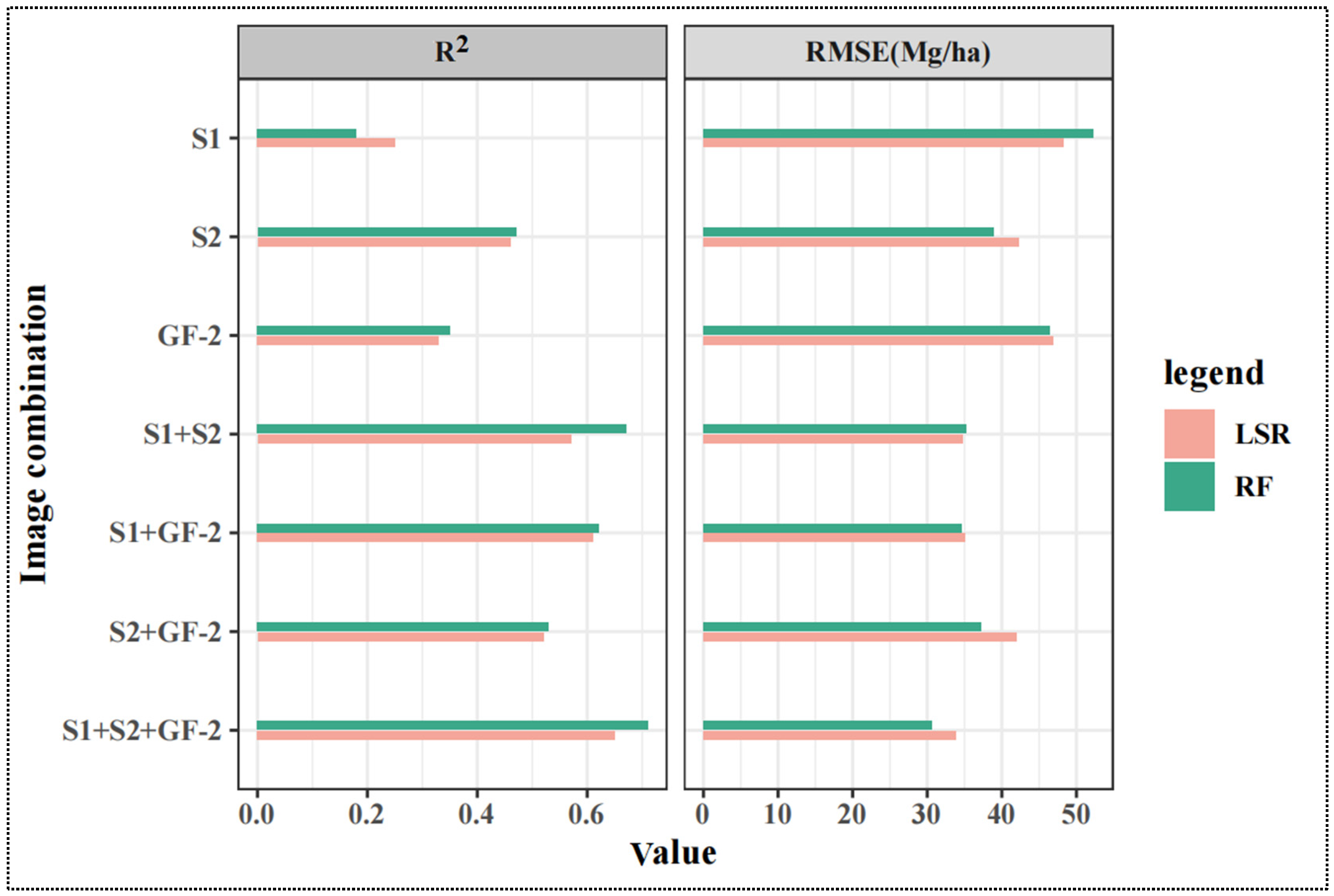
Following the stepwise regression variable screening, 19 variables were chosen for model construction. These variables encompassed 3 vegetation indices, 13 texture features, and 2 band combinations. Only images captured in the VH polarization mode were included in our modeling strategy. The predictors involved in the modeling are provided in

Table 3. Selected variables from various sensors.

Sensor	Variables
S1	S1_VH
S2	S2_CON_b12_3 × 3, S2_REP, S2_ASM_b8_3 × 3, S2_COR_b2_3 × 3, S2_ME_b2_9 × 9
GF-2	GF_CON_b4_7 × 7, GF_EN_b4_7 × 7, GF_DI_b4_7 × 7, GF-B23, GF_ASM_b1_5 × 5, GF_EN_b1_5 × 5, GF_DI_b1_5 × 5
S1 + S2	S2_REP, S2_ME_b5_9 × 9, S2_GNDVI, S2_ASM_b8_3 × 3, S2_RVI, S1_VH, S2_COR_b2_3 × 3
S1 + GF-2	GF_VA_b4_7 × 7, GF_CON_b4_7 × 7, S1_VH, GF_B13
S2 + GF-2	S2_REP, S2_COR_b2_3 × 3, GF_B13, S2_CON_b12_3 × 3, S2_ME_b2_9 × 9
S1 + S2 + GF-2	S2_REP, GF_VA_b2_5 × 5, S2_RVI, S2_NDVI, S2_ME_b5_9 × 9, S2_ASM_b8_3 × 3, S1_VH, S2_COR_b2_3 × 3, GF-B23

.

After selecting variables step by step, RF is used to sort different remote sensing variables, as shown in Figure 3. Only VH appeared in S1. Of the S2 variables, the S2_REP variable was the most important. Among the GF-2 variables, the most important were GF_CON_b4_7 × 7, GF_DI_b4_7 × 7, and GF_EN_b1_5 × 5. In the S1 + S2 variable combination, the S2_REP and S2_ME_b5_9×9 variables were the most important. In the S1 + GF-2 variable combination, the variable importance ranks as follows: GF_VA_b4_7 × 7, GF_CON_b4_7 × 7, S1_VH, and GF_B13. When the S2 + GF-2 variables were combined, S2_REP and S2_COR_b2_3 × 3 were more important. Among the three variable combinations, the top three variables ranked in order of importance were GF-B13, GF_VA_b2_5 × 5, and S2_REP.

3.2. Model Fitting

Drawing from the correlation analysis between forestAGB and the independent variables, the variables utilized in the stepwise regression process are detailed in Table 3. The stepwise regression model obtained after linear stepwise fitting is shown in

Table 4. Construction of LSR model.

Group	Expressions
S1	Y = 289.684 + 11.979 × S1_VH
S2	Y = − 2.437 × 105 + 3.457 × 102 × S2_REP − 22.55 × S2_COR_b2_3 × 3 + 42.12 × S2_CON_b12_3 × 3 + 8.705 × S2_ME_b2_9 × 9 − 23.96 × S2_ASM_b8_3 × 3
GF-2	Y = − 152.2074 + 45.2420 × GF-B23 + 78.4102 × GF_EN_b1_5 × 5 + 0.1851 × GF_DI_b1_5 × 5 + 10.5578 × GF_CON_b4_7 × 7 − 74.0780 × GF_DI_b4_7 × 7
S1 + S2	Y = − 3.778 × 105 + 8.578 × S1_VH + 5.362 × 102 × S2_REP − 54.14 × S2_RVI + 1.077 × 102 × S2_GNDVI − 17.30 × S2_COR_b2_3 × 3 − 23.86 × S2_ASM_b8_3 × 3 + 36.99 × S2_ME_b5_9 × 9
S1 + GF-2	Y = 205.099 + 10.880 × S1_VH + 7.770 × GF_CON_b4_7 × 7 + 21.239 × GF_B13 − 9.367 × GF_VA_b4_7 × 7
S2 + GF-2	Y = − 2.175 × 105 + 3.086 × 102 × S2_REP − 24.42 × S2_COR_b2_3 × 3 + 42.90 × S2_CON_b12_3 × 3 + 19.11 × GF_B13 + 8.594 × S2_ME_b2_9 × 9
S1 + S2 + GF-2	Y = − 3.469 × 105 + 8.099 × S1_VH + 4.924 × 102 × S2_REP − 69.48 × S2_RVI + 1.015 × 102 × S2_NDVI − 19.98 × S2_COR_b2_3×3 + 32.58 × GF-B23 + 3.659 × GF_VA_b2_5 × 5 − 23.15 × S2_ASM_b8_3 × 3 + 34.24 × S2_ME_b5_9 × 9

.

The outcomes of the 10-fold cross-validation process are presented in Figure 4. The modeling accuracy of the AGB using single remote-sensing data was compared. The ranges of R² were from 0.18 to 0.47, with the accuracy of the S1 LSR model being 0.25, with an RMSE of 48.33 Mg/ha. These values surpassed those derived from the RF model constructed with AGB using S1 (R² = 0.18, RMSE = 52.30 Mg/ha). For the S2 image, the LSR model had an R² of 0.46 with an RMSE of 42.29 Mg/ha, which is smaller than that of the RF model (R² = 0.47, RMSE = 38.98 Mg/ha). In the case of the GF-2 image, the RF model yielded an R² value of 0.35 and an RMSE of 46.45 Mg/ha, whereas the LSR model attained an R² of 0.33 and an RMSE of 46.81 Mg/ha. In terms of modeling accuracy, S2 was the best, having more spectral information and more vegetation indices, while GF-2 was the second best, having the highest possible resolution, which was better able to reflect the vegetation, while S1 was the worst due to the shorter C-band, which did not reflect the comprehensive spatial information of the forest well.

This demonstrates that combining S1, S2, and GF-2 yielded an R² of 0.71 and a RMSE of 30.67 Mg/ha using the RF model and a 0.65 R² with 33.79 Mg/ha RMSE for the LSR model (Figure 4). The S1 + S2 blend was the runner-up in forecasting the forest AGB, securing a 0.67 R² and a 35.26 Mg/ha RMSE in the RF model, and a 0.57 R² with a 34.70 Mg/ha RMSE in the LSR model. Under the S1 + GF-2 combination, the R² and RMSE of the RF model were 0.62 and 34.07 Mg/ha, and the R² and RMSE of the LSR model were 0.61 and 35.57 Mg/ha, respectively. Under the S2 + GF-2 condition, there was no notable distinction observed in the R² or RMSE values between the LSR and RF models. To sum up, the combined use of optical and SAR satellite data showcased the utmost precision, boasting an R² value of 0.71 and an RMSE of 30.67 Mg/ha. Thus, the model utilizing both optical and SAR data demonstrated superior accuracy. These findings indicate that integrating remote-sensing images, particularly combining optical and SAR data, is crucial for significantly enhancing AGB estimation accuracy.

3.3. Mapping

Figure 5 illustrates the mapping outcomes of forest biomass estimation derived from individual remote sensing sources (S1, S2, GF-2), as well as the amalgamation of multiple remote sensing sources (S1 + S2, S1 + GF-2, S2 + GF-2, and S1 + S2 + GF-2) within the Yuanmou dry-hot valley region obtained via remote sensing techniques. From Figure 5, it is evident that the inversion outcomes for the seven cases exhibited a similar distribution pattern for both high and low AGB values. The single remote-sensing estimations gave mainly low values, the heterogeneity was poor, and there may have been a serious underestimation of high values, with the S1 heterogeneity and sensitivity being the worst. For the combined images, the S1 + S2 + GF-2 combination had high heterogeneity and sensitivity, whereas S2 + GF-2 was the worst. Overall, the AGB estimation results indicate that the greatest amount of biomass was found in the south and east of Yuanmou, with the smallest amount mainly being concentrated in the foothills and alongside river valleys with lower elevations and slopes. Leveraging multiple remote sensing sources proved to be more effective than solely relying on individual remote sensing datasets. The results obtained from combining S1, S2, and GF-2 (S1 + S2 + GF-2) were particularly meaningful for understanding the biomass distribution in this region.

4. Discussion

4.1. Importance Analysis of the Variables

After sorting the RF variables based on their importance, it was found that VH had high importance in the backscattering coefficient of S1. Manh Van Pham’s [26] study also showed that the VH model had a good fitting effect with the multiple linear regression model [26]. Among the S2 variables, S2_NDVI, S2_REP, S2_RVI, and S2_GNDVI all contained red-edge bands in the planting coverage index, with the red-edge bands having a more significant effect on vegetation monitoring [16]. The GNDVI estimates that the AGB potential of dryland forests is greater than that of the NDVI. This finding aligns with the results reported in the study conducted by David et al. [65]. Among the GF-2 variables, GF-B23 and GF_B13 contributed significantly to the estimation of forest AGB. In addition, 12 variables were selected from the texture features, indicating that these were important contributors to the estimation of AGB. Earlier research has also indicated the significant contribution of texture features in forest AGB estimation [66,67].

4.2. Single Remote-Sensing Comparison

Our findings revealed that S2 gave the highest performance in estimating forest AGB when considering single remotely sensed data, with the RF model recording an R² of 0.47 and an RMSE of 38.93 Mg/ha, while the LSR model had an R² of 0.46 and RMSE of 42.29 Mg/ha. The forest AGB estimation accuracy derived from the S2 data exceeded that from the GF-2 and S1 (SAR) data [33,68]. The excellent performance of the S2 data can be attributed to its relatively high spatial resolution and rich band information. Texture details and vegetation indices from the S2 data have been shown to notably enhance its performance [69,70]. Another important factor was that the 10 m × 10 m resolution of the S2 images matched the 10 × 10-m ground sample plots we used, thus theoretically eliminating the presence of mixed pixels. Consequently, the high temporal and spatial resolution multi-spectral data of S2 gave a better estimation accuracy. The GF-2 data gave poor results in the forest AGB estimation, even though GF-2 theoretically had a higher resolution. However, we resampled the GF-2 data, which resulted in a loss of spectral information. Resampling inevitably changes the information content of the image and introduces pixel localization and geometric accuracy errors [70]. In addition, there may have been more single-attribute pixels in a single pixel of the GF-2 data. This scaling phenomenon may result in estimation inaccuracies across various spatial resolutions [70]. The S1 data gave the worst estimation performance. This may be because the C-band is affected by complex terrain in rugged mountainous areas, thus affecting its ability to improve AGB estimations [33,71]. However, this might be due to the fact that the acquisition of remote-sensing data coincided with the region’s rainy season, leading to increased environmental humidity. Studies have demonstrated that backscattering intensity is also influenced by ambient temperature and humidity [72,73,74]. Yu and Saatchi [75] used L-band backscattering characteristics to observe 11 different forest biomes worldwide. They noted that the relationship between L-band backscattering and AGB may be significantly influenced by forest type and environment. In addition, this study did not incorporate the texture features of S1 into the test. Recent comparative studies have found that the texture information of S1 makes a better contribution to forest AGB [76,77]. The effectiveness of texture information will be further explored in future studies.

4.3. Combination Comparison

In our study, the AGB model combining the S1, S2, and GF-2 imagery had higher estimation accuracy than using S1, S2, or GF-2 imagery alone. Integrating variable factors from diverse remote-sensing data sources can offer a more comprehensive description of the data. The integration of optical and SAR data showed the advantage of the acquisition of both vegetation spectral traits and canopy structure information [69,76,77]. As shown in Figure 4, the S1 SAR and optical data (S2, GF-2) gave the best performance in forest biomass estimation in the Yuanmou area, with the RF model obtaining the highest R² (0.71), which was better than for the combinations S1 + S2, S1 + GF-2 or S2 + GF-2, proving that integrating all the different types of sensors improved the estimation significantly. Backscattering can improve the retrieval of forest parameters [27]. Our findings align with those of Zhu et al. [34], who effectively estimated the forest AGB of China’s largest artificial mangrove forest by integrating GF-2, GF-3 SAR, and unmanned aerial vehicle DSM data, yielding optimal results.

Moreover, multi-source data can be used effectively on a global scale. Hu et al. [78] used multiple data to make a global forest AGB map with a spatial resolution of 1 km for the first time, which is in good agreement with other published AGB distributions. Prior research has indicated that integrating SAR data with other types of data enhances forest AGB estimation, particularly when combined with optical imagery [52,69]. This discrepancy can be ascribed to variations in imaging methodologies, data attributes, and informational richness across the systems (e.g., SAR provides structural information, whereas optical data provide canopy density and vegetation condition information) [33]. We found that in combination with the SAR polarization values, S1 + S2 and S1 + GF-2 produced better estimations than S2 + GF-2. Other studies using S1 and S2 data for AGB estimation have obtained similar results. Naidoo et al. [79] showed that integrating S1 and S2 data enhanced the precision of forest AGB estimation in contrast to relying on a single sensor. Ignoring S2 and integrating S1 and GF-2, the two models can estimate forest AGB well and the results are not dissimilar. The R² of the RF model was 0.01 higher than that of the LSR model, and the RMSE was 0.5 Mg/ha lower. These results show that the integration of optical data and SAR data can simultaneously obtain the advantages of vegetation spectral characteristics and canopy structure information. Our study shows that the integration of different remote-sensing datasets produces better results than using a single remote-sensing dataset. Fang et al. [80] had similar results to those from our study, with multi-sensor combinations outperforming single sensors and, in most cases, non-parametric models outperforming parametric models. Non-parametric models are more widely used. David et al. [65] used S1 and S2 to estimate the AGB of a national park in a tropical savannah forest and adopted the RF algorithm to obtain the best performance model, with the R² value reaching 0.95. This is better than the RF estimation effect of combining S1 and S2 found in our study, which may be affected by different regions and terrain. Li et al. [81] integrated the remote-sensing images from GF-2 and S2, effectively harnessing these data to enhance the precision of coniferous forest stock volume estimation. Using four different remote-sensing images, they demonstrated that fusion images based on GF-2 and S2 could improve forest stock volume estimation performance and provide new insights for optical image fusion and adaptive modeling [82]. In our next study, we will explore the estimation effect of image fusion in forest AGB. The combination of S1, S2, and GF-2 imagery used in our study provides new insights into the complementary nature of multi-source imagery for more accurate future forest AGB estimations in different woodland areas in dry-hot valley regions.

4.4. Limitations and Future Research

The dry-hot valley we studied is mainly situated in the Hengduan Mountain region of Southwestern China. The valley is deep, the topographic heterogeneity is high, the climate is hot and dry, and the vertical zonal differentiation of the natural environment is obvious [83]. Although the topography, vegetation, and climate of dry-hot river valleys are similar, the methodological system used in our study has not yet been used to estimate the forest biomass in other dry-hot river valleys. We intend to extend the method to other dry-hot river valley areas that may have different forest types or environmental conditions to further evaluate its effectiveness. This will help to verify the applicability and reliability of the method and provide a wider range of applications for future research.

Although combining multiple remote-sensing data sources gave a relatively higher forest AGB estimation accuracy, several limitations persisted when employing remote sensing for AGB estimation. Sensor errors, such as atmospheric correction and noise, and spatial resolution errors, including cloud cover and mountain shadow, will cause detail loss, while spectral resolution errors will affect optical data acquisition, complex terrain and ground object mixing errors will lead to ground object misjudgment, all of which will cause errors [6]. Although some errors cannot be avoided completely, we should minimize them to improve the accuracy and reliability of AGB estimation. In future studies, we will incorporate factors, such as spatial information, a DEM, temperature, precipitation, and other SAR data with longer bands, into the model. We will study higher-resolution DEM data for SAR terrain correction. The rise of various models and different algorithms, such as machine learning, deep learning, U2net, Yolo, etc., are widely used in forest firefighting, the medical Internet of Things, target detection, and other fields [84,85,86,87]. We will explore their applications in forestry while investigating trends in forest AGB over time to assess forest health and the value of deforestation. In addition, we will explore alternative data sources, like lidar and UAVs, to enhance forest AGB estimation accuracy.

5. Conclusions

It is crucial to investigate how accurately forest AGB estimation fits when employing a combination of diverse remote-sensing data in dry-hot valley regions. Here, 78 plots, located in Yuanmou County, Yunnan Province, China, were sampled for ground data that were then compared to remote-sensing data from one active and two passive sources. To compare the fitting effects of the parametric and non-parametric models, LSR and RF models were constructed. These led to the following findings:

• The combination of the GF-2, S1, and S2 remote-sensing datasets improved the estimation performance of forest AGB, the estimation effect being in the order S1 + S2 + GF-2 > SI + S2>S1 + GF-2 > S2 + GF-2, with S1 + S2 + GF-2 having the best prediction effect, containing tectonic information from the horizontal and vertical lines. With both their high resolution and multiple bands, the three different sensors provided richer information. These findings demonstrate that combining optical and SAR images can enhance estimation accuracy.
• The RF gave the best fitting performance compared to the LSR for all four combinations (S1 + S2 + GF-2, S1 + S2, S1 + GF-2, S2 + GF-2), with the R² and RMSE values for both evaluation models being 0.71 and 0.65, and 30.67 and 33.79 Mg/ha, respectively.

In conclusion, the precision of forest biomass retrieval by combining optical remote-sensing images and SAR data is better than that of a single dataset. The estimation methods presented here can help forest resource managers better understand structure and biomass, and thus develop more effective conservation and management strategies. Accurate estimates of forest biomass can provide important data for the calculation of carbon emissions and absorption, help assess the impact of forests on climate change, and offer a scientific foundation for the development of pertinent policies.

References

1. Achard, F.; Eva, H.D.; Stibig, H.-J.; Mayaux, P.; Gallego, J.; Richards, T.; Malingreau, J.-P. Determination of deforestation rates of the world’s humid tropical forests. Science 2002, 297, 999–1002. [Google Scholar] [CrossRef] [PubMed]
2. Dong, J.; Kaufmann, R.K.; Myneni, R.B.; Tucker, C.J.; Kauppi, P.E.; Liski, J.; Buermann, W.; Alexeyev, V.; Hughes, M.K. Remote sensing estimates of boreal and temperate forest woody biomass: Carbon pools, sources, and sinks. Remote Sens. Environ. 2003, 84, 393–410. [Google Scholar] [CrossRef]
3. Huang, H.; Liu, C.; Wang, X.; Zhou, X.; Gong, P. Integration of multi-resource remotely sensed data and allometric models for forest aboveground biomass estimation in China. Remote Sens. Environ. 2019, 221, 225–234. [Google Scholar] [CrossRef]
4. Gibbs, H.K.; Brown, S.; Niles, J.O.; Foley, J.A. Monitoring and estimating tropical forest carbon stocks: Making REDD a reality. Environ. Res. Lett. 2007, 2, 045023. [Google Scholar] [CrossRef]
5. Goetz, S.J.; Baccini, A.; Laporte, N.T.; Johns, T.; Walker, W.; Kellndorfer, J.; Houghton, R.A.; Sun, M. Mapping and monitoring carbon stocks with satellite observations: A comparison of methods. Carbon Balance Manag. 2009, 4, 2. [Google Scholar] [CrossRef] [PubMed]
6. Lu, D. The potential and challenge of remote sensing-based biomass estimation. Int. J. Remote Sens. 2006, 27, 1297–1328. [Google Scholar] [CrossRef]
7. Lu, D.; Chen, Q.; Wang, G.; Liu, L.; Li, G.; Moran, E. A survey of remote sensing-based aboveground biomass estimation methods in forest ecosystems. Int. J. Digit. Earth 2016, 9, 63–105. [Google Scholar] [CrossRef]
8. Ou, G.; Lv, Y.; Xu, H.; Wang, G. Improving forest aboveground biomass estimation of Pinus densata forest in Yunnan of Southwest China by spatial regression using Landsat 8 images. Remote Sens. 2019, 11, 2750. [Google Scholar] [CrossRef]
9. Yadav, S.A.; Prasad, R.; Srivastava, P.K.; Singh, S.K.; Sharma, J.; Khamrai, S. Time-series polarimetric bistatic scattering decomposition using comprehensive modified first-order radiative transfer model at C-band for vegetative terrain and validation. Int. J. Remote Sens. 2022, 43, 7161–7180. [Google Scholar] [CrossRef]
10. Luo, J.; Dong, C.; Lin, K.; Chen, X.; Zhao, L.; Menzel, L. Mapping snow cover in forests using optical remote sensing, machine learning and time-lapse photography. Remote Sens. Environ. 2022, 275, 113017. [Google Scholar] [CrossRef]
11. Huang, J.-C.; Ko, K.-M.; Shu, M.-H.; Hsu, B.-M. Application and comparison of several machine learning algorithms and their integration models in regression problems. Neural Comput. Appl. 2020, 32, 5461–5469. [Google Scholar] [CrossRef]
12. Santoro, M.; Cartus, O.; Carvalhais, N. The global forest above-ground biomass pool for 2010 estimated from high-resolution satellite observations. Earth Syst. Sci. Data Discuss. 2020, 2020, 1–38. [Google Scholar] [CrossRef]
13. Yun, J.; Qian, S.S. A hierarchical model for estimating long-term trend of atrazine concentration in the surface water of the contiguous US. JAWRA J. Am. Water Resour. Assoc. 2015, 51, 1128–1137. [Google Scholar] [CrossRef]
14. Papathanassiou, K.; Cloude, S.; Pardini, M.; Quiñones, M.; Hoekman, D.; Ferro-Famil, L.; Goodenough, D.; Chen, H.; Tebaldini, S.; Neumann, M. Forest applications. In Polarimetric Synthetic Aperture Radar: Principles and Application; Springer: Cham, Switzerland, 2021; pp. 59–117. [Google Scholar]
15. Ashourloo, D.; Shahrabi, H.S.; Azadbakht, M.; Rad, A.M.; Aghighi, H.; Radiom, S. A novel method for automatic potato mapping using time series of Sentinel-2 images. Comput. Electron. Agric. 2020, 175, 105583. [Google Scholar] [CrossRef]
16. Karlson, M.; Ostwald, M.; Bayala, J.; Bazié, H.R.; Ouedraogo, A.S.; Soro, B.; Sanou, J.; Reese, H. The potential of Sentinel-2 for crop production estimation in a smallholder agroforestry landscape, Burkina Faso. Front. Environ. Sci. 2020, 8, 85. [Google Scholar] [CrossRef]
17. Gou, R.-K.; Chen, J.-Q.; Duan, G.-H.; Yang, R.; Bu, Y.-K.; Zhao, J.; Zhao, P.-X. Inversion of aboveground biomass of Pinus tabuliformis plantations based on GF-2 data. Ying Yong Sheng Tai Xue Bao/J. Appl. Ecol. 2019, 30, 4031–4040. [Google Scholar]
18. Li, X.; Liu, Z.; Lin, H.; Wang, G.; Sun, H.; Long, J.; Zhang, M. Estimating the growing stem volume of Chinese pine and larch plantations based on fused optical data using an improved variable screening method and stacking algorithm. Remote Sens. 2020, 12, 871. [Google Scholar] [CrossRef]
19. Wang, Z.; Yi, L.; Xu, W.; Zheng, X.; Xiong, S.; Bao, A. Integration of UAV and GF-2 Optical Data for Estimating Aboveground Biomass in Spruce Plantations in Qinghai, China. Sustainability 2023, 15, 9700. [Google Scholar] [CrossRef]
20. Amuyou, U.A.; Wang, Y.; Ebuta, B.F.; Iheaturu, C.J.; Antonarakis, A.S. Quantification of Above-Ground Biomass over the Cross-River State, Nigeria, Using Sentinel-2 Data. Remote Sens. 2022, 14, 5741. [Google Scholar] [CrossRef]
21. Moradi, F.; Sadeghi, S.M.M.; Heidarlou, H.B.; Deljouei, A.; Boshkar, E.; Borz, S.A. Above-ground biomass estimation in a Mediterranean sparse coppice oak forest using Sentinel-2 data. Ann. For. Res. 2022, 65, 165–182. [Google Scholar] [CrossRef]
22. Frampton, W.J.; Dash, J.; Watmough, G.; Milton, E.J. Evaluating the capabilities of Sentinel-2 for quantitative estimation of biophysical variables in vegetation. ISPRS J. Photogramm. Remote Sens. 2013, 82, 83–92. [Google Scholar] [CrossRef]
23. Attarchi, S.; Gloaguen, R. Improving the estimation of above ground biomass using dual polarimetric PALSAR and ETM+ data in the Hyrcanian mountain forest (Iran). Remote Sens. 2014, 6, 3693–3715. [Google Scholar] [CrossRef]
24. Santoro, M.; Beer, C.; Cartus, O.; Schmullius, C.; Shvidenko, A.; McCallum, I.; Wegmüller, U.; Wiesmann, A. Retrieval of growing stock volume in boreal forest using hyper-temporal series of Envisat ASAR ScanSAR backscatter measurements. Remote Sens. Environ. 2011, 115, 490–507. [Google Scholar] [CrossRef]
25. Cartus, O.; Santoro, M.; Wegmüller, U.; Labrière, N.; Chave, J. Sentinel-1 coherence for mapping above-ground biomass in semiarid forest areas. IEEE Geosci. Remote Sens. Lett. 2021, 19, 1–5. [Google Scholar] [CrossRef]
26. Van Pham, M.; Pham, T.M.; Du, Q.V.V.; Bui, Q.-T.; Van Tran, A.; Pham, H.M.; Nguyen, T.N. Integrating Sentinel-1A SAR data and GIS to estimate aboveground biomass and carbon accumulation for tropical forest types in Thuan Chau district, Vietnam. Remote Sens. Appl. Soc. Environ. 2019, 14, 148–157. [Google Scholar] [CrossRef]
27. Liang, P.; Pierce, L.E.; Moghaddam, M. Radiative transfer model for microwave bistatic scattering from forest canopies. IEEE Trans. Geosci. Remote Sens. 2005, 43, 2470–2483. [Google Scholar] [CrossRef]
28. Coops, N.C.; Tompalski, P.; Goodbody, T.R.; Achim, A.; Mulverhill, C. Framework for near real-time forest inventory using multi source remote sensing data. Forestry 2023, 96, 1–19. [Google Scholar] [CrossRef]
29. Zhang, R.; Zhou, X.; Ouyang, Z.; Avitabile, V.; Qi, J.; Chen, J.; Giannico, V. Estimating aboveground biomass in subtropical forests of China by integrating multisource remote sensing and ground data. Remote Sens. Environ. 2019, 232, 111341. [Google Scholar] [CrossRef]
30. Wang, J.; Xiao, X.; Bajgain, R.; Starks, P.; Steiner, J.; Doughty, R.B.; Chang, Q. Estimating leaf area index and aboveground biomass of grazing pastures using Sentinel-1, Sentinel-2 and Landsat images. ISPRS J. Photogramm. Remote Sens. 2019, 154, 189–201. [Google Scholar] [CrossRef]
31. Hudak, A.T.; Lefsky, M.A.; Cohen, W.B.; Berterretche, M. Integration of lidar and Landsat ETM+ data for estimating and mapping forest canopy height. Remote Sens. Environ. 2002, 82, 397–416. [Google Scholar] [CrossRef]
32. Zhang, C.; Denka, S.; Cooper, H.; Mishra, D.R. Quantification of sawgrass marsh aboveground biomass in the coastal Everglades using object-based ensemble analysis and Landsat data. Remote Sens. Environ. 2018, 204, 366–379. [Google Scholar] [CrossRef]
33. Forkuor, G.; Zoungrana, J.-B.B.; Dimobe, K.; Ouattara, B.; Vadrevu, K.P.; Tondoh, J.E. Above-ground biomass mapping in West African dryland forest using Sentinel-1 and 2 datasets-A case study. Remote Sens. Environ. 2020, 236, 111496. [Google Scholar] [CrossRef]
34. Zhu, Y.; Liu, K.; Myint, S.; Du, Z.; Li, Y.; Cao, J.; Liu, L.; Wu, Z. Integration of GF2 optical, GF3 SAR, and UAV data for estimating aboveground biomass of China’s largest artificially planted mangroves. Remote Sens. 2020, 12, 2039. [Google Scholar] [CrossRef]
35. Shettles, M.; Temesgen, H.; Gray, A.N.; Hilker, T. Comparison of uncertainty in per unit area estimates of aboveground biomass for two selected model sets. For. Ecol. Manag. 2015, 354, 18–25. [Google Scholar] [CrossRef]
36. Wang, G.; Zhang, M.; Gertner, G.Z.; Oyana, T.; McRoberts, R.E.; Ge, H. Uncertainties of mapping aboveground forest carbon due to plot locations using national forest inventory plot and remotely sensed data. Scand. J. For. Res. 2011, 26, 360–373. [Google Scholar] [CrossRef]
37. Karlson, M.; Ostwald, M.; Reese, H.; Sanou, J.; Tankoano, B.; Mattsson, E. Mapping tree canopy cover and aboveground biomass in Sudano-Sahelian woodlands using Landsat 8 and random forest. Remote Sens. 2015, 7, 10017–10041. [Google Scholar] [CrossRef]
38. Huang, T.; Ou, G.; Wu, Y.; Zhang, X.; Liu, Z.; Xu, H.; Xu, X.; Wang, Z.; Xu, C. Estimating the Aboveground Biomass of Various Forest Types with High Heterogeneity at the Provincial Scale Based on Multi-Source Data. Remote Sens. 2023, 15, 3550. [Google Scholar] [CrossRef]
39. Zald, H.S.; Wulder, M.A.; White, J.C.; Hilker, T.; Hermosilla, T.; Hobart, G.W.; Coops, N.C. Integrating Landsat pixel composites and change metrics with lidar plots to predictively map forest structure and aboveground biomass in Saskatchewan, Canada. Remote Sens. Environ. 2016, 176, 188–201. [Google Scholar] [CrossRef]
40. Peng, S.; Chen, A.; Fang, H.; Wu, J.; Liu, G. Effects of vegetation restoration types on soil quality in Yuanmou dry-hot valley, China. Soil Sci. Plant Nutr. 2013, 59, 347–360. [Google Scholar] [CrossRef]
41. Zhenzhou, J. A phytosociological study on the semi-savanna vegetation in the dry-hot valleys of Yuanjiang River, Yunnan. Guangxi Zhiwu 1999, 19, 289–302. [Google Scholar]
42. Tang, X.; Zhao, X.; Bai, Y.; Tang, Z.; Wang, W.; Zhao, Y.; Wan, H.; Xie, Z.; Shi, X.; Wu, B. Carbon pools in China’s terrestrial ecosystems: New estimates based on an intensive field survey. Proc. Natl. Acad. Sci. USA 2018, 115, 4021–4026. [Google Scholar] [CrossRef] [PubMed]
43. Decker, B.L. World Geodetic System 1984; Defense Mapping Agency Aerospace Center: St Louis, MO, USA, 1986. [Google Scholar]
44. Luo, Y.; Wang, X.; Ouyang, Z.; Lu, F.; Feng, L.; Tao, J. A review of biomass equations for China’s tree species. Earth Syst. Sci. Data 2020, 12, 21–40. [Google Scholar] [CrossRef]
45. Xu, H.Z.; Ou, G.; Shi, H. A study on Estimation and Distribution for Forest Biomass and Carbon Storage in Yun-Nan Province. Chin. Agric. Sci. Bull. 2019, 12, 21–40. [Google Scholar]
46. Qin, Q.; Xu, D.; Hou, L.; Shen, B.; Xin, X. Comparing vegetation indices from Sentinel-2 and Landsat 8 under different vegetation gradients based on a controlled grazing experiment. Ecol. Indic. 2021, 133, 108363. [Google Scholar] [CrossRef]
47. Zheng, G.; Chen, J.; Tian, Q.; Ju, W.; Xia, X. Combining remote sensing imagery and forest age inventory for biomass mapping. J. Environ. Manag. 2007, 85, 616–623. [Google Scholar] [CrossRef] [PubMed]
48. Haralick, R.M. Statistical and structural approaches to texture. Proc. IEEE 1979, 67, 786–804. [Google Scholar] [CrossRef]
49. Hashemi, S.A.; Fallah Chai, M.M.; Bayat, S. An analysis of vegetation indices in relation to tree species diversity using by satellite data in the northern forests of Iran. Arab. J. Geosci. 2013, 6, 3363–3369. [Google Scholar] [CrossRef]
50. Miura, T.; Huete, A.; Yoshioka, H. An empirical investigation of cross-sensor relationships of NDVI and red/near-infrared reflectance using EO-1 Hyperion data. Remote Sens. Environ. 2006, 100, 223–236. [Google Scholar] [CrossRef]
51. Schlerf, M.; Atzberger, C.; Hill, J. Remote sensing of forest biophysical variables using HyMap imaging spectrometer data. Remote Sens. Environ. 2005, 95, 177–194. [Google Scholar] [CrossRef]
52. Cutler, M.; Boyd, D.S.; Foody, G.M.; Vetrivel, A. Estimating tropical forest biomass with a combination of SAR image texture and Landsat TM data: An assessment of predictions between regions. ISPRS J. Photogramm. Remote Sens. 2012, 70, 66–77. [Google Scholar] [CrossRef]
53. Jiang, F.; Kutia, M.; Ma, K.; Chen, S.; Long, J.; Sun, H. Estimating the aboveground biomass of coniferous forest in Northeast China using spectral variables, land surface temperature and soil moisture. Sci. Total Environ. 2021, 785, 147335. [Google Scholar] [CrossRef]
54. Jiang, F.; Kutia, M.; Sarkissian, A.J.; Lin, H.; Long, J.; Sun, H.; Wang, G. Estimating the growing stem volume of coniferous plantations based on random forest using an optimized variable selection method. Sensors 2020, 20, 7248. [Google Scholar] [CrossRef] [PubMed]
55. Zheng, S.; Cao, C.; Dang, Y.; Xiang, H.; Zhao, J.; Zhang, Y.; Wang, X.; Guo, H. Retrieval of forest growing stock volume by two different methods using Landsat TM images. Int. J. Remote Sens. 2014, 35, 29–43. [Google Scholar] [CrossRef]
56. O’brien, R.M. A caution regarding rules of thumb for variance inflation factors. Qual. Quant. 2007, 41, 673–690. [Google Scholar] [CrossRef]
57. Eguiguren, P.; Ojeda Luna, T.; Torres, B.; Lippe, M.; Günter, S. Ecosystem service multifunctionality: Decline and recovery pathways in the amazon and chocó lowland rainforests. Sustainability 2020, 12, 7786. [Google Scholar] [CrossRef]
58. Fassnacht, F.; Hartig, F.; Latifi, H.; Berger, C.; Hernández, J.; Corvalán, P.; Koch, B. Importance of sample size, data type and prediction method for remote sensing-based estimations of aboveground forest biomass. Remote Sens. Environ. 2014, 154, 102–114. [Google Scholar] [CrossRef]
59. Li, Y.; Li, C.; Li, M.; Liu, Z. Influence of variable selection and forest type on forest aboveground biomass estimation using machine learning algorithms. Forests 2019, 10, 1073. [Google Scholar] [CrossRef]
60. Breiman, L. Random forests. Mach. Learn. 2001, 45, 5–32. [Google Scholar] [CrossRef]
61. Cutler, D.R.; Edwards Jr, T.C.; Beard, K.H.; Cutler, A.; Hess, K.T.; Gibson, J.; Lawler, J.J. Random forests for classification in ecology. Ecology 2007, 88, 2783–2792. [Google Scholar] [CrossRef]
62. Belgiu, M.; Drăguţ, L. Random forest in remote sensing: A review of applications and future directions. ISPRS J. Photogramm. Remote Sens. 2016, 114, 24–31. [Google Scholar] [CrossRef]
63. Pelletier, C.; Valero, S.; Inglada, J.; Champion, N.; Dedieu, G. Assessing the robustness of Random Forests to map land cover with high resolution satellite image time series over large areas. Remote Sens. Environ. 2016, 187, 156–168. [Google Scholar] [CrossRef]
64. Shekar, B.; Dagnew, G. Grid search-based hyperparameter tuning and classification of microarray cancer data. In Proceedings of the 2019 Second International Conference on Advanced Computational and Communication Paradigms (ICACCP), Gangtok, India, 25–28 February 2019; pp. 1–8. [Google Scholar]
65. David, R.M.; Rosser, N.J.; Donoghue, D.N. Improving above ground biomass estimates of Southern Africa dryland forests by combining Sentinel-1 SAR and Sentinel-2 multispectral imagery. Remote Sens. Environ. 2022, 282, 113232. [Google Scholar] [CrossRef]
66. Lu, D.; Batistella, M. Explorando texturas de imagens TM e suas relações com estimativas de biomassa em Rondônia. Acta Amaz. 2005, 35, 249–257. [Google Scholar] [CrossRef]
67. Pandit, S.; Tsuyuki, S.; Dube, T. Exploring the inclusion of Sentinel-2 MSI texture metrics in above-ground biomass estimation in the community forest of Nepal. Geocarto Int. 2020, 35, 1832–1849. [Google Scholar] [CrossRef]
68. Castillo, J.A.A.; Apan, A.A.; Maraseni, T.N.; Salmo, S.G., III. Estimation and mapping of above-ground biomass of mangrove forests and their replacement land uses in the Philippines using Sentinel imagery. ISPRS J. Photogramm. Remote Sens. 2017, 134, 70–85. [Google Scholar] [CrossRef]
69. Vafaei, S.; Soosani, J.; Adeli, K.; Fadaei, H.; Naghavi, H.; Pham, T.D.; Tien Bui, D. Improving accuracy estimation of Forest Aboveground Biomass based on incorporation of ALOS-2 PALSAR-2 and Sentinel-2A imagery and machine learning: A case study of the Hyrcanian forest area (Iran). Remote Sens. 2018, 10, 172. [Google Scholar] [CrossRef]
70. Adan, M.S. Integrating Sentinel-2 Derived Vegetation Indices and Terrestrial Laser Scanner to Estimate Above-Ground Biomass/Carbon in Ayer Hitam Tropical Forest Malaysia. Master’s Thesis, University of Twente, Enschede, The Netherlands, 2017. [Google Scholar]
71. Laurin, G.V.; Liesenberg, V.; Chen, Q.; Guerriero, L.; Del Frate, F.; Bartolini, A.; Coomes, D.; Wilebore, B.; Lindsell, J.; Valentini, R. Optical and SAR sensor synergies for forest and land cover mapping in a tropical site in West Africa. Int. J. Appl. Earth Obs. Geoinf. 2013, 21, 7–16. [Google Scholar]
72. Nguyen, L.V.; Tateishi, R.; Nguyen, H.T.; Sharma, R.C.; To, T.T.; Le, S.M. Estimation of tropical forest structural characteristics using ALOS-2 SAR data. Adv. Remote Sens. 2016, 5, 131–144. [Google Scholar] [CrossRef]
73. Touzi, R.; Deschamps, A.; Rother, G. Wetland characterization using polarimetric RADARSAT-2 capability. Can. J. Remote Sens. 2007, 33, S56–S67. [Google Scholar] [CrossRef]
74. Kasischke, E.S.; Bourgeau-Chavez, L.L.; Rober, A.R.; Wyatt, K.H.; Waddington, J.M.; Turetsky, M.R. Effects of soil moisture and water depth on ERS SAR backscatter measurements from an Alaskan wetland complex. Remote Sens. Environ. 2009, 113, 1868–1873. [Google Scholar] [CrossRef]
75. Yu, Y.; Saatchi, S. Sensitivity of L-band SAR backscatter to aboveground biomass of global forests. Remote Sens. 2016, 8, 522. [Google Scholar] [CrossRef]
76. Chen, L.; Ren, C.; Zhang, B.; Wang, Z.; Xi, Y. Estimation of forest above-ground biomass by geographically weighted regression and machine learning with sentinel imagery. Forests 2018, 9, 582. [Google Scholar] [CrossRef]
77. Navarro, J.A.; Algeet, N.; Fernández-Landa, A.; Esteban, J.; Rodríguez-Noriega, P.; Guillén-Climent, M.L. Integration of UAV, Sentinel-1, and Sentinel-2 data for mangrove plantation aboveground biomass monitoring in Senegal. Remote Sens. 2019, 11, 77. [Google Scholar] [CrossRef]
78. Hu, T.; Su, Y.; Xue, B.; Liu, J.; Zhao, X.; Fang, J.; Guo, Q. Mapping global forest aboveground biomass with spaceborne LiDAR, optical imagery, and forest inventory data. Remote Sens. 2016, 8, 565. [Google Scholar] [CrossRef]
79. Naidoo, L.; Van Deventer, H.; Ramoelo, A.; Mathieu, R.; Nondlazi, B.; Gangat, R. Estimating above ground biomass as an indicator of carbon storage in vegetated wetlands of the grassland biome of South Africa. Int. J. Appl. Earth Obs. Geoinf. 2019, 78, 118–129. [Google Scholar] [CrossRef]
80. Fang, G.; Xu, H.; Yang, S.-I.; Lou, X.; Fang, L. Synergistic use of Sentinel-1, Sentinel-2, and Landsat 8 in predicting forest variables. Ecol. Indic. 2023, 151, 110296. [Google Scholar] [CrossRef]
81. Li, X.; Lin, H.; Long, J.; Xu, X. Mapping the growing stem volume of the coniferous plantations in North China using multispectral data from integrated GF-2 and Sentinel-2 images and an optimized Feature variable selection method. Remote Sens. 2021, 13, 2740. [Google Scholar] [CrossRef]
82. Li, X.; Long, J.; Zhang, M.; Liu, Z.; Lin, H. Coniferous plantations growing stock volume estimation using advanced remote sensing algorithms and various fused data. Remote Sens. 2021, 13, 3468. [Google Scholar] [CrossRef]
83. Zhang, W.; Liu, L.; Song, K.; Li, X.; Wang, Y.; Tang, Y.; Jiang, H. Remote sensing the orographic effects of dry-hot valley on vegetation distribution in the southeast Tibetan Plateau. Int. J. Remote Sens. 2019, 40, 8589–8607. [Google Scholar] [CrossRef]
84. Zhang, Y.; Ma, J.; Liang, S.; Li, X.; Li, M. An evaluation of eight machine learning regression algorithms for forest aboveground biomass estimation from multiple satellite data products. Remote Sens. 2020, 12, 4015. [Google Scholar] [CrossRef]
85. Phan, D.T.; Yap, K.-H.; Garg, K.; Han, B.S. Vision-Based Early Fire and Smoke Detection for Smart Factory Applications Using FFS-YOLO. In Proceedings of the 2023 IEEE 25th International Workshop on Multimedia Signal Processing (MMSP), Kuala Lumpur, Malaysia, 27–29 September 2023; pp. 1–6. [Google Scholar]
86. Phan, D.T.; Nguyen, C.H.; Nguyen, T.D.P.; Tran, L.H.; Park, S.; Choi, J.; Lee, B.-I.; Oh, J. A flexible, wearable, and wireless biosensor patch with internet of medical things applications. Biosensors 2022, 12, 139. [Google Scholar] [CrossRef] [PubMed]
87. Phan, D.T.; Ta, Q.B.; Ly, C.D.; Nguyen, C.H.; Park, S.; Choi, J.; Se, H.O.; Oh, J. Smart low level laser therapy system for automatic facial dermatological disorder diagnosis. IEEE J. Biomed. Health Inform. 2023, 27, 1546–1557. [Google Scholar] [CrossRef] [PubMed]
Figure 1. Flowchart describing the research procedure.
Forests 15 00731 g001
Figure 2. Study area overview maps showing: (a) the geographic position of Yunnan Province within China; (b) the location of Yuanmou County, Yunnan Province; and (c) the sample sites in Yuanmou County.
Forests 15 00731 g002
Figure 3. Ranking of RF variable importance.
Forests 15 00731 g003
Figure 4. Modeling results for the image combinations.
Forests 15 00731 g004
Figure 5. Forest AGB estimations for Yuanmou County using various remote-sensing sensors: (a) inverted map from S1; (b) inverted map from S2; (c) inverted map from GF-2; (d) inverted map from S1 + S2; (e) inverted map from S1 + GF-2; (f) inverted map from S2 + GF-2; and (g) inverted map from S1 + S2 + GF-2.
Forests 15 00731 g005