
Revealing the Effect of Typhoons on the Stability of Residual Soil Slope by Wind Tunnel Test
by
Zizheng Guo
1, 
Yuanbo Liu
1,
Taili Zhang
2,*,
Juehao Zhang
1,
Haojie Wang
1,
Jun He
1,3,
Guangming Li
4 and
Bixia Tian
1 1
School of Civil and Transportation Engineering, Hebei University of Technology, Tianjin 300401, China
2
Nanjing Center of the China Geological Survey, Nanjing 210016, China
3
Faculty of Geo-Information Science and Earth Observation (ITC), University of Twente, 7522 NH Enschede, The Netherlands
4
Tianjin Municipal Engineering Design & Research Institute (TMEDI), Tianjin 300392, China
*
Author to whom correspondence should be addressed.
Forests 2024, 15(5), 791; https://doi.org/10.3390/f15050791
Submission received: 24 March 2024
/
Revised: 20 April 2024
/
Accepted: 25 April 2024
/
Published: 30 April 2024
(This article belongs to the Special Issue Impacts of Extreme Climate Events on Forests)
Abstract
:Typhoon-induced slope failure is one of the most important geological hazards in coastal areas. However, the specific influence of typhoons on the stability of residual soil slopes still remains an open issue. In this study, the Feiyunjiang catchment in Zhejiang Province of SE China was chosen as the study area, and a downscaling physical model of residual soil slopes in the region was used to carry out the wind tunnel test. Our aim was to answer the question, How does the vegetation on the slope and slope stability respond during a typhoon event? For this purpose, multiple aspects were monitored and observed under four different wind speeds (8.3 m/s, 10.3 m/s, 13.3 m/s, and 17 m/s), including vegetation damage on the slope, macrocracks on the slope surface, wind pressure, wind load, permeability coefficient of the soil layer, and slope stability. The results showed that the plants on the slope could restore to their original states when the wind speeds ranged from 8.3 m/s to 13.3 m/s, but were damaged to the point of toppling when the wind speed increased to 17 m/s. Meanwhile, evident cracks were observed on the ground under this condition, which caused a sharp increase in the soil permeability coefficient, from 1.06 × 10⁻⁵ m/s to 6.06 × 10⁻⁴ m/s. The monitored wind pressures were larger at the canopy than that at the trunk for most of the trees, and generally larger at the crown of the slope compared with the toe of the slope. Regarding the wind load to the slope ground, the total value increased significantly, from 35.4 N under a wind speed of 8.3 m/s to 166.5 N under a wind speed of 17 m/s. However, the wind load presented different vector directions at different sections of the slope. The quantitative assessment of slope stability considering the wind load effect revealed that the safety factor decreased by 0.123 and 0.1 under the natural state and saturated state, respectively, from no wind to a 17 m/s strong wind. Overall, the present results explained the mechanism of slope failure during typhoon events, which provided theoretical reference for revealing the characteristics of residual soil slope stability under typhoon conditions.
1. Introduction
Coastal regions often suffer from typhoons in rainy seasons [1,2]. During a typhoon, strong winds and heavy rainfall commonly trigger slope failures, which can cause considerable damage to society and the environment [3,4]. East Asia is a rainstorm-triggered landslide-prone area all over the world, with more than 10% of the fatal landslides occurring in China, according to statistical results [5,6]. For example, the catastrophic Su village landslide triggered by a typhoon rainstorm caused 27 deaths, and more than 20 houses were destroyed in September 2016 in Zhejiang Province, China, although the volume was only 0.4 million m3 [7]. Hence, it is very important to investigate the impact of typhoons on slope stability, especially for soil slopes.
SE China faces the Pacific Ocean; therefore, it is often affected by monsoon and tropical cyclones in summer on a yearly basis [8]. Some literature has revealed the considerable disadvantages of the typhoon-induced landslides in the region, which are mainly relevant to the aspects of water and wind erosion for soils [9,10], the fatal damages of landslides to residents [11], and the destructive significance of typhoons for the economy and society [12]. Current studies regarding typhoon-triggered landslides mainly focus on the occurrence mechanism [13], rainfall infiltration process and threshold [14], event-based inventory construction [15], and regional spatial modeling and analysis [16,17,18]. The applied methods are generally associated with field work and monitoring [19,20], numerical simulation [21], remote sensing, and GIS techniques [22,23]. However, these studies mainly emphasize the effect of heavy rainfall during typhoons and commonly ignore the role of wind [24]. The wind is a common driver of forest disturbance [25,26], and its controlling effect on geomorphology can be basically summarized as follows: First, trees can transfer dynamic-wind force as a turning moment to the soil layer, which can result in tree toppling or throwing [27]. Second, wind can also concentrate the precipitation amount, which is originally modulated by elevation and aspect [28]. Meanwhile, wind can destroy trees to produce advantageous seepage channels [29]. However, the specific role of wind in inducing landslides has remained an open issue until now, and the cause-and-effect relationship is unclear. Particularly, how to quantitatively assess the impacts of wind on slope failure is an operational challenge for scientists.
Given that the direct measurement of the effect of wind on slope is commonly complex, researchers often explore the joint effect of typhoons, rainfall, and trees on landslide initiation in coastal regions [30]. For example, Parra et al. [31] applied a hierarchical Bayesian logistic regression to investigate the role of forest cover and wind speed in landslide prediction in Patagonian. Zhuang et al. [32] proposed a numerical model that involves typhoon wind load, preferential infiltration, and root reinforcement, which calculated wind load through a combination of the autoregressive method and a multi-degree-of-freedom tree swaying mode. Moreover, researchers have widely explored methods to quantitatively assess the stabilizing effect of vegetation on slopes. The methods include, but not limited to, the physical model [33,34], the rainfall infiltration model [18,35], and laboratory tests [36]. However, as Rulli et al. [27] concluded, studies on the internal mechanism between slope hydrology and wind-driven forest disturbance are rather rare, especially when it comes to the landslide prediction model. Additionally, in the present literature regarding landslide susceptibility assessment on the regional scale, few studies employed land cover as an analysis factor in the model [30,37].
In this context, we aim to reveal the effect of typhoons on the stability of residual soil slope in this study. Specifically, our objectives include: (i) monitoring and calculating the wind pressure and wind load during strong winds with different velocities to slope surface and vegetation by designing a laboratory physical model test, and observing the condition of the damaged plants on the slope; (ii) checking macrocracks on the ground after wind with different velocities and measuring permeability coefficient of the soil layer; (iii) calculating the residual thrust and safety factor by considering wind load effect to quantitatively assess the slope stability under strong winds.
2. Description of the Study Area
In this study, the Feiyun River catchment in Zhejiang Province of SE China was selected as the study area (Figure 1). The total length of the river is 203 km, with a total area of 3252 km2. The landform of the whole area is mainly low mountains and hills, with higher elevation in the southwest and lower elevation in the northeast on the overall topography. The mountainous area in the southwest has a greatly undulating terrain, the eastern area is mostly plain, and the river network is dense. Geologically, the tectonic system mainly includes NNE and NW fault zones, and the lithology is mainly mudstone and sandstone of the Moshishan Group of Upper Jurassic and the Yongkang Group of Lower Cretaceous. Moreover, metamorphic rock from Upper Paleozoic exists locally. Regarding the climate regime, the Feiyun River catchment has a central subtropical maritime monsoon climate with an average annual rainfall of around 1870 mm, and a maximum to minimum rainfall ratio of about 2.1.
Because the study area is located on the coast of the Pacific Ocean, it is often hit by typhoons in the summer [38]. As shown in Figure 2, at least 15 typhoons landed in the region during 2002 and 2016, and the maximum wind speeds of these events ranged from 25 m/s to 65 m/s, with four greater than 60 m/s and only one below 30 m/s. The durations of the typhoons were mostly in the range of 10 to 60 h. These typhoon and rainstorm events often induce landslide episodes, resulting in a large number of casualties and property losses. The typhoon-triggered landslides mainly occurred in residual soil or strongly weathered soil layers, on a small scale in many cases, most of which were shallow earth slides or earth flows with volume less than 104 m3. The slope failure can be characterized as tensile cracks on the crown, water seepage at the toe of the slope, and vegetation toppling.
3. Implementation of the Wind Tunnel Model Test
3.1. Principle of the Test and Parameter Determination
In order to simulate the effects of typhoon conditions on slope vegetation and its stability, a typical residual soil landslide in the study area was reduced on an equal scale and then subjected to wind tunnel simulation tests. The experiment was essentially a physical model test and therefore followed the principle of quantitative analysis, i.e., only physical quantities of the same type were subjected to mathematical operations [39,40]. When performing a similar ratio analysis, the variables consisted of two main categories, namely internal and external factors. Physical-mechanical parameters were the main internal factors affecting slope deformation, and a total of 10 internal factors were considered in this study, including slope dimension l, inclination angle θ, density ρ, cohesion c, friction angle φ, deformation modulus E, Poisson’s ratio μ, gravitational acceleration g, stress σ, and strain ε. The external factors mainly involved parameters related to typhoons and vegetation, including wind speed ν, duration t, vegetation height, and cover. According to the similarity ratio principle, if C was defined as the ratio of the prototype’s actual parameters to the model parameters, the similarity ratios of the above parameters were Cl = n, Cθ = 1, Cρ = 1, Cc = n, CΦ = 1, CE = n, Cμ = n, Cg = 1, Cσ = n, Cε = n, Cν = , and Ct = . It should be noted that there is no agreement regarding the similarity ratio (scale) for wind speed between the real condition and experiment conditions in the science community [41]. However, according to the literature review [41,42], the settings in this study were considered suitable.
According to the results of the field investigation and indoor test, the values of the parameters of the prototype slope are shown in Table 1. Four grades of typhoon speeds were set in this test according to the standard of China National Meteorological Administration; that is, v was 33 m/s, 41 m/s, 53 m/s, and 65 m/s, respectively. By referring to the previous literature, the similarity ratio n was determined to be 16, and thus, the final slope model parameter values were obtained (Table 1). The corresponding wind speeds under different situations were 8.3 m/s, 10.3 m/s, 13.3 m/s, and 17 m/s, respectively, and the wind and slope direction were set at 90°. Considering the time similarity coefficient Ct = 4 and the general conditions of the experimental equipment, the experimental time for each group was set to 1 h.
3.2. Physical Model Design
A triangular model box of 1.38 × 1.0 × 0.8 m (length, width, and height) was made with a steel frame, with Plexiglas panels for the side walls and construction wood panels for the bottom serving as the interface between bedrock and sliding body [43]. It should be noted that slope failure is normally a shallow landslide caused by a typhoon, so the slope model can be simplified as an infinite slope [44]. This means that there was empty space between the support construction and the box bottom. The slope material was a mixture of river sand, expansive soil, clay, and barite powder. Through experimental adjustment, it was determined that the physical and mechanical parameters of the slope material fitted well with Table 1 when the ratio of the four materials was 39:10:39:12. The above materials were compacted and shaped in the model box. There are two main plants in the study area, namely bamboos and shrubs. However, the former normally have shallow roots, which have limited effects on slope stability under typhoon conditions. Hence, in order to observe the behavior of slope failure under typhoons more closely, only shrubs were used as plants in this study. Fake plants were made using plastic, with a height of 0.15 m and root depth of 0.6 m. In total, 12 model trees were arranged on the surface of the model, with four rows and three columns (Figure 3a,b). The distance between adjacent trees was 0.4 m from left to right and 0.3 m from front to back, with a crown diameter of about 0.3 m. The total shadow area of these trees covered approximately 80% of the slope surface, which fit well with the coverage degree of the area. Next, plastic film was used to cover the model surface to prevent the generation of suspended particles due to excessive wind speed and vegetation destruction. A schematic diagram of the final slope model is shown in Figure 3c.
3.3. Test Instruments and Setting
In this study, the instruments were developed in the wind tunnel laboratory of Central South University, China, including a high-frequency electronic pressure scanning valve, a micropressure sensor, and a dynamic data acquisition system. Three wind pressure monitoring points (①, ②, ③) were arranged on the ground of the toe, middle part, and the top of the slope, respectively. For each monitoring point, two wind pressure monitoring pipes were placed in parallel at an interval of 1 cm. Moreover, for the 12 trees on the slope, three wind pressure monitoring pipes were also set up with a height of 0.1, 0.2, and 0.35 m to the ground, respectively (Figure 4a). A total of 42 monitoring pipes were connected to the pressure scanning valve on the back side of the model to collect wind pressure data every 5 min. The collected data were subsequently imported into a notebook computer through the wind pressure monitoring system for analysis (Figure 4b).
3.4. Data Collection and Processing
This study carried out four wind tunnel experiments by setting different wind speeds, and the following data were monitored and analyzed:
- (i)
- Vegetation: Taking photos of the vegetation on the slope after each group of experiments, and recording their details, including the dumping number, inclination direction, and angle.
- (ii)
- Crack development: Recording the details of the cracks on the slope surface after each group of experiments, including number, length, and width.
- (iii)
- Wind pressure and wind load: Monitoring and recording wind pressure values on the ground and on the trees. As shown in Figure 5a, the model slope was divided into three profiles for comparison and analysis. After obtaining the wind pressure data of the trees, the MATLAB R2020b software was used to desiccate and thin the data to produce the curves of wind pressure with time for each model tree at different heights. The positive values represented the pressure effect, while the negative values represented the suction effect. To facilitate the calculation of wind load, each tree was divided into three wind pressure zones, namely A, B, and C (Figure 5b). The wind pressure values in these zones were represented by the monitoring data from points a, b, and c (Figure 4a). Moreover, the wind pressure values on the slope surface were represented by the data from the monitoring point on the ground. The wind load value of each area was calculated by multiplying the wind pressure with the force area.
- (iv)
- Permeability coefficient: At the end of each set of experiments, in situ soil samples were taken at the top of the slope location using an iron cylinder, followed by an indoor infiltration test. The cylinders had a diameter of 15 cm and a height of 20 cm, and each sample was taken at a depth of 15 cm. Darcy’s law was used to design the infiltration test [45,46]. An in situ soil sample was placed on a sump with a 2 cm high sidewall, and the sump was filled with water both at the top and at the bottom of the sample. When the sump began to overflow, the sample was left in the sump for an hour. Meanwhile, the upper boundary was filled with water every five minutes, and the amount of water added was calculated. When the amount of water was stabilized, the permeability coefficient of the soil sample was obtained using Darcy’s law.
- (v)
- Slope stability: In order to analyze and compare the effect of wind on the sliding force and slope stability under different situations, the residual thrust [47] and safety factor were calculated.
The traditional residual thrust method only considers the sliding force and friction force due to the self-weight of the slide body, and the effect of cohesion on the slide surface [48], which is as follows:
where WH and WZ are the gravitational forces of the slide and vegetation, respectively; L is the length of the slide, c is the cohesion of soil, φ is the friction angle of soil, and a is the slope angle of the slide surface. Under the effect of a strong wind, the residual thrust of the slope (Figure 6) can be expressed as follows:
where FP is the wind load on the slope surface, and FZ and FZ1 are the wind loads applied to the vegetation and its reaction force on the slide, respectively. When the reserve of slope stability is considered, the residual sliding force of the slope can be obtained by dividing the slip resistance value by the safety factor Fs:
E = WHsinα − WHcosα-cL
E = (WH + WZ)sinα + FZ1cosα − [(WH + WZ)cosαtanφ + cL + Fptanφ − FZ1sinαtanφ]
E = (WH + WZ)sinα + FZ1cosα−[(WH + WZ)cosαtanφ + cL + Fptanφ − FZ1sinαtanφ]/Fs
The initial Fs is entered into the above equation and then calibrated continuously according to the value of the residual sliding force. When the residual sliding force is 0, the FS at this time can be determined as the final slope stability.
4. Results and Discussion
4.1. Vegetation Damage
The damage to vegetation under typhoon action in each situation is shown in Figure 7. It can be found that the vegetation finally returned to an upright position at wind speeds of 8.3 m/s, 10.3 m/s, and 13.4 m/s (Figure 7a–c), and obvious deformation was not observed on the rest of the model. However, at a wind speed of 17 m/s, the vegetation on the slope was significantly tilted and several cracks were observed on the ground (Figure 7d). This indicated that a wind speed greater than 17 m/s could cause evident slope failure in residual soil and thus damage vegetation.
4.2. Analysis of Wind Pressure
Figure 8, Figure 9 and Figure 10 show the wind pressure variation of different profiles under wind with a speed of 8.3 m/s. It was found that wind pressures were generally larger at the tree canopy, and the largest values were observed for trees #12 and #6. All the trees had wind pressure values around 35 Pa at the canopy, except trees #3 (−2.5 Pa) and #9 (0 Pa). Regarding the position of the tree trunk, wind pressure on profiles 1 and 3 gradually decreased from the foot to the crown of the slope. All of them had positive wind pressures at the foot of the slope and negative wind pressures at the crown of the slope, and their values were between −15 and 25 Pa. The wind pressure of tree trunk #11 was the largest, at about 50 Pa, and the smallest, at about 0 Pa, for trees #2 and #8. The wind pressure values at the bottom of the trunk varied similarly to those at the middle of the trunk.
When the wind speed increased to 10.3 m/s (Supplementary Figures S1–S3), the wind pressure at the tree canopy was still the highest. In particular, trees #2, #6, and #12 had the largest values, ranging from about 70 to 90 Pa, and tree #3 had a negative value of −5 Pa, which was the smallest. At the tree trunk, the maximum wind pressure on profiles 1 and 3 occurred at tree #7 (22.5 Pa) and tree #9 (50 Pa), respectively, and the minimum wind pressure occurred at the top of the slope at tree #1 (−20 Pa) and tree #3 (−5 Pa), respectively. For profile 2, the maximum wind pressure was 80 Pa at tree #11 at the foot of the slope, and the minimum value was 2 Pa for tree #8. The variation of wind pressure at the bottom of the trunk was similar to that under a wind speed of 8.3 m/s. The maximum wind pressure of tree #11 was −5 Pa, which was basically similar to the wind speed of 8.3 m/s. The minimum value was −5 Pa for tree #11. The wind pressure at the bottom of the trunk varied similarly to that of the wind speed of 8.3 m/s, with the largest wind pressure value at tree #11 (75 Pa), the smallest value at tree #8 (−100 Pa), and the rest of the values distributed between −15 and 15 Pa.
Under the wind with a speed of 13.4 m/s (Supplementary Figures S4–S6), trees #2 and #6 had the largest wind pressure values of about 135 Pa, and the values for the rest were around 100 Pa except trees #3 (5 Pa) and #9 (20 Pa). At the trunk, the wind pressure showed the maximum values at the foot of the slope and the minimum values at the top of the slope, except tree #10 (−60 Pa) and tree #6 (−20 Pa). The bottom of the trunk was similar to the middle of the trunk, with wind pressure values being maximum at the foot of the slope and minimum at the top of the slope, with a maximum of 130 Pa for tree #11 and a minimum of −70 Pa for tree #9.
Under the wind with a speed of 17 m/s (Supplementary Figures S7–S9), the wind pressure variation was generally similar to the wind speed of 8.3 m/s. At the canopy, trees #2, #3, and #12 had the largest wind pressure, between 160 and 180 Pa, except tree #5 (30 Pa) and tree #6 (5 Pa). At the trunk, the largest value of wind pressure was for tree #11 (170 Pa), while tree #10 in the same row had the smallest value of wind pressure (−75 Pa). Trees #1, #3, #6, and #10 showed negative wind pressures for suction, with an average of around −25 Pa. The bottom of the trunk for profiles 1 and 3 were the largest at the foot of the slope and the smallest in the row above it, while profile 2 showed the largest in the second row at the foot of the slope and the smallest at the top of the slope, where the largest wind pressure was for tree #8 (200 Pa) and the smallest for tree #6 (−90 Pa).
However, one single tree may not play a big role during natural conditions. Therefore, to better reveal the characteristics of wind pressure and different sections, the statistical results for the selected profiles and sections were also analyzed. When the wind speed was 8.3 m/s, for the different parts of the slope model, the average wind pressure was 8.2 kPa (top part, #1, #2, and #3), 39.5 kPa (middle part, #4~#9), and 101.6 kPa (toe part, #10, #11, and #12), respectively. When the wind speed was the largest (17m/s), the average wind pressure increased to 175.2 kPa (top part, #1, #2, and #3), 330.6 kPa (middle part, #4~#9), and 332.3 kPa (toe part, #10, #11, and #12), respectively. For the different profiles, profile 1 (#1, #4, #7, and #10) had an average wind pressure of 36.8 kPa when the wind was 8.3 m/s, whereas the values for profile 2 (#2, #5, #8, and #11) and profile 3 (#3, #6, #9, and #12) were 46.6 kPa and 56.3 kPa, respectively. When the wind speed increased to 17 m/s, the average wind pressure reached 165.8 kPa (profile 1), 259.5 kPa (profile 2), and 202.4 kPa (profile 3), respectively. These results can lead us to conclude that the wind pressure at the slope bottom was the largest, and that for the middle and right parts was larger than that for the left profile.
4.3. Analysis of Wind Load
The calculated wind load values imposed on the 12 trees at different wind speeds are shown in Figure 11. We can see that the total wind load on the slope was 35.4 N at a wind speed of 8.3 m/s, with a wind load value of each single tree being less than 5 N (Figure 11a). For the trees of each profile, the wind loads decreased from bottom to top. However, this was not the case for the trees in the tope row (trees #1, #2, and #3). This is because they were subjected to the direct action of the wind due to higher elevation, with less blocking effect from the other trees. As shown in Figure 11b, the wind load with a wind speed of 10.3 m/s was greater than that of the first group, but the load on each tree was less than 10 N. The two rows of trees at the top part of the slope were subjected to a slightly greater wind load overall than that at the bottom part of the slope, while the second row of trees in the windward direction was subjected to the smallest wind load. The total value of the wind load on the vegetation of the slope was 58.3 N. Regarding the results with a wind speed of 13.4 m/s (Figure 11c), the highest wind load was observed at the top of the slope, followed by the trees at the bottom of the slope. The two rows of trees in the middle of the slope had smaller wind load values. The total wind load on the slope increased to 112.73 N. When the wind speed was set at 17 m/s (Figure 11d), the trees on the top part of the slope still had the highest wind load values, and the first and second rows of trees received slightly smaller wind loads. The third row of trees was observed to have the smallest value of wind load, which was close to 0. The total value of wind load on the slope was the highest among all the situations, reaching 166.5 N.
Second, to compare the wind load at different locations of the slope, the curves showing the wind loads at different zones are presented in Figure 12. Zones ①, ②, and ③ have been defined in Figure 5. When the wind speed was 8.3 m/s (Figure 12a), the value of wind load on zone ② was smaller than that on zone ①, and the wind load on zone ③ was negative. This indicates that the toe and the middle of the slope were subjected to the pressure of the wind load towards the slope interior, while the top area of the slope was subjected to the suction of the wind load towards the outside of the slope. The calculation of curve integration reveals that the total wind load on the modeled slope was −0.9 N. Similar to the last situation, the toe of the slope still received the largest wind load (33 N/m) when the wind speed was 10.3 m/s (Figure 12b), followed by the middle region of the slope with a smaller wind load (15 N/m), and the top region of the slope had a negative value of wind load (−22 N/m). The total wind load on the slope increased to 3.5 N. When the wind speed was 13.4 m/s (Figure 12c), the maximum value of wind load was 60 N/m in zone ①, the value of wind load in zone ② was about 24 N/m, and the wind load in zone ③ was −38 N/m. The total wind load on the slope was 5.2 N. The wind load on the modeled slope was 5.2 N. The results at a wind speed of 17 m/s are shown in Figure 12d. It can be found that the wind loads were evidently higher in this situation, namely 80 N/m (zone ①), 38 N/m (zone ②), and −57 N/m (zone ③), respectively. The total wind load on the slope was also the highest, at 8 N.
4.4. Permeability Coefficient and Stability
According to the experiment workflow introduced in Section 3.4, the permeability coefficients of the slope for the initial situation (no wind) and after the four experimental conditions (strong wind) were measured. The results showed that the permeability coefficient without wind was 1.06 × 10⁻⁵ m/s. When the wind speed increased from 8.3 m/s to 13.4 m/s, no obvious deformation or damage occurred to the slope, and the permeability coefficients remained nearly constant. However, under a strong wind with a speed of 17 m/s, the permeability coefficient changed evidently, increasing to 6.06 × 10⁻⁴ m/s. This fit well with the macro deformation of the slope, which was mainly characterized by the toppling of the trees at the top of the slope, and the deformation of the root resulted in the creation of soil fissures. This behavior caused a significant increase in the soil permeability.
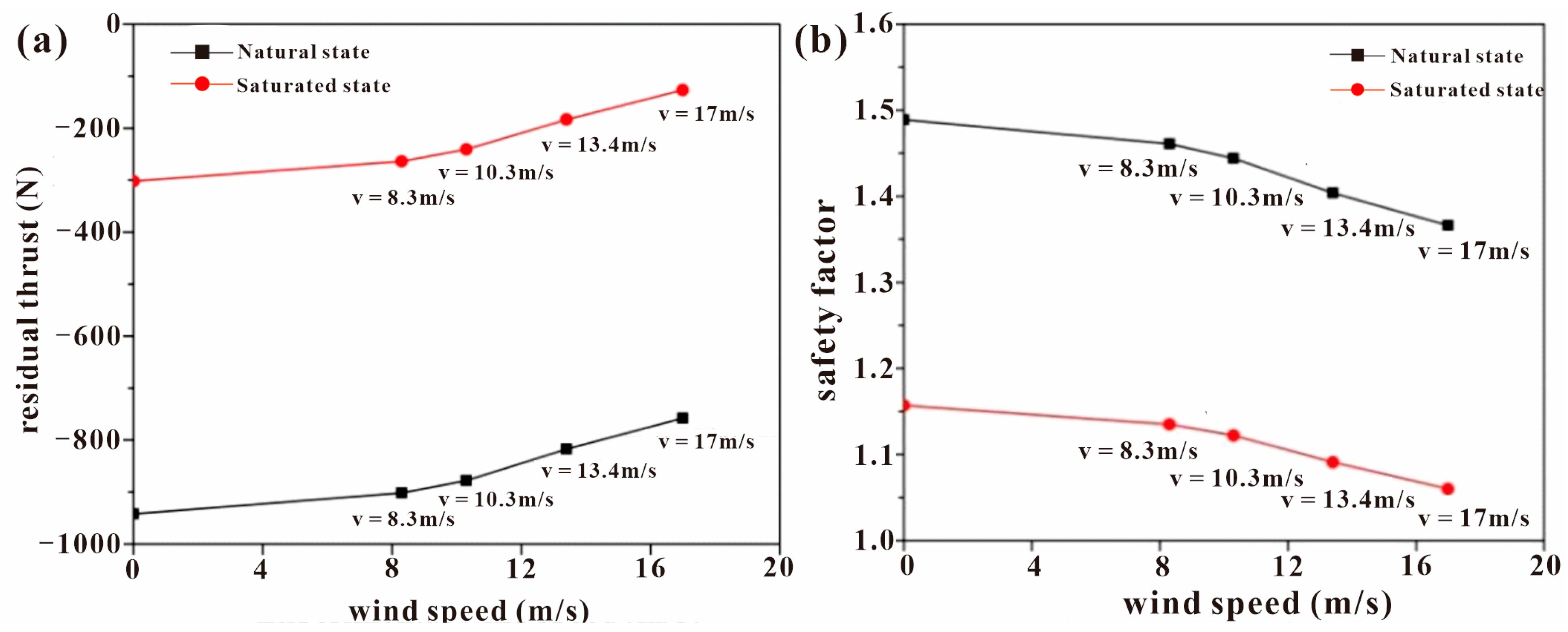
Given that residual soil slopes are generally in a saturated state during typhoon rainstorms [49,50], their stability under two conditions was calculated in this study, namely natural state and saturated state. The physical-mechanical parameters of soil and the wind loads on the vegetation and the slope body were introduced into Equations (2) and (3), respectively, to obtain the residual thrust and safety factor of the slope under the action of different wind speeds. As seen in Figure 13a, the residual thrust of the model in the natural state without wind was −942.1 N, and the safety factor was 1.49 (Figure 13b). As the wind speed increased in the experiment, the sliding force of the slope gradually increased and the safety factor decreased. When the wind speed reached 17 m/s, the safety factor of the slope decreased by 0.123 compared with the initial condition. However, the typhoon load was not enough to cause instability due to the good initial stability of the model in the natural state. When it came to the saturated state, the residual thrust force without wind was −302.0 N, and the safety factor was 1.16. This result indicated that the slope stability at this time was poor and only remained stable basically. When the wind speed was 13.4 m/s, the slope stability had already decreased below 1.1, and reached 1.06 after the wind speed increased to 17 m/s, which revealed that the model was close to the critical value of instability.
4.5. Limitations and Future Works
The size of the model box was determined based on the scale between the box and the real slope, which took the law of similarity as the theoretical foundation. The scale was set as 16 because the model size (0.15–1.56 m in Table 1) under this condition is suitable for a laboratory test. For example, if the scale is 8, the geometric size of the model will be 0.3–3.12 m, which is a little large for a manmade model. On the other hand, it should be noted that the scale effect from the model box may affect the observed results, but it is complex to quantify its effects [40,51]. Sensitivity analysis of size is a potential resolution but is not possible in the current study, given its economic costs.
Another limitation of the experiment is its validation. The results from the laboratory physical model were directly considered as the real results without verification by field observations. This may result in uncertainties. However, the in-site experiment may be rather complicated, including drilling and monitoring, etc., and the wind conditions should also fit well with the test settings. Some previous studies [40,52] also lacked this procedure, which makes us believe that the field survey and observations can inherit the results from the model test.
5. Conclusions
In this study, we investigated the quantitative effect of strong wind on the behavior of vegetated residual soil slope by applying a downscaling physical model. The observed results showed that vegetation, ground crack, wind pressure on vegetation, wind load on the ground, the permeability coefficient of soil, and stability of the slope varied with wind speed. When the wind speed was less than 13.4 m/s, the plants on the slope could restore to their original states after the wind, and the permeability coefficient of soil nearly did not change compared with the initial condition. However, evident failure was monitored on plants on the slope when the wind speed was 17 m/s. Meanwhile, the permeability coefficient of soil increased largely, which led to rainfall infiltration more quickly. The quantitative calculation considering the wind load effect indicated that the safety factor of the slope decreased by 0.123 and 0.1 under natural state and saturated state, respectively, from no wind to a 17 m/s strong wind. This resulted in the slope being close to instability under a saturated state with a safety factor of 1.06, because the initial stability was lower under this condition.
Overall, the present results provided evidence of the joint role of strong wind and precipitation in landslide initiation, and the response of slope stability behavior may have a close relationship with wind speed. Hence, it seems important to find a speed threshold to determine the probability of typhoon-triggered landslide occurrence.
Supplementary Materials
The following supporting information can be downloaded at: https://www.mdpi.com/article/10.3390/f15050791/s1, Figure S1: Wind pressure variation curves for each tree on profile 1 at a wind speed of 10.3 m/s; Figure S2: Wind pressure variation curves for each tree on profile 2 at wind speed 10.3 m/s; Figure S3: Wind pressure variation curves for each tree on profile 3 at wind speed 10.3 m/s; Figure S4: Wind pressure variation curves for each tree on profile 1 at a wind speed of 13.4 m/s; Figure S5: Wind pressure variation curves for each tree on profile 2 at a wind speed of 13.4 m/s; Figure S6: Wind pressure variation curves for each tree on profile 3 at a wind speed of 13.4 m/s; Figure S7: Wind pressure variation curves for each tree on profile 1 at a wind speed of 17 m/s; Figure S8: Wind pressure variation curves for each tree on profile 2 at a wind speed of 17 m/s; Figure S9: Wind pressure variation curves for each tree on profile 3 at a wind speed of 17 m/s.
Author Contributions
Conceptualization, Z.G., T.Z., H.W. and J.H.; methodology, Z.G., Y.L., T.Z., J.Z. and J.H; software, Y.L., J.Z. and H.W.; validation, T.Z., J.Z. and J.H.; formal analysis, Z.G., Y.L., H.W. and J.H.; investigation, Y.L., T.Z., J.Z. and J.H.; resources, Z.G. and T.Z; data curation, Y.L., T.Z., H.W. and J.H; writing—original draft preparation, Z.G. and Y.L.; writing—review and editing, T.Z., G.L. and B.T.; visualization, H.W.; supervision, Z.G. and J.Z.; project administration, H.W.; funding acquisition, Z.G., T.Z. and G.L. All authors have read and agreed to the published version of the manuscript.
Funding
This research is funded by the Natural Key R&D Program of China (2022YFC3003200), geological survey projects of the Feiyun River catchment of Zhejiang (DD20160282), and the Planning and Natural Resources Research Project of Tianjin City (2022-40, KJ [2024]25). Bixia Tian wants to thank the support from the Graduated Student Innovation Funding Project of Hebei Province (CXZZSS2024007).
Data Availability Statement
The data presented in this study are available on request from the corresponding author.
Conflicts of Interest
The authors declare no conflicts of interest. The funders had no role in the design of the study; in the collection, analyses, or interpretation of data; in the writing of the manuscript; or in the decision to publish the results.
References
- Abancó, C.; Bennett, G.L.; Matthews, A.J.; Matera, M.A.M.; Tan, F.J. The role of geomorphology, rainfall and soil moisture in the occurrence of landslides triggered by 2018 Typhoon Mangkhut in the Philippines. Nat. Hazards Earth Syst. Sci. 2021, 21, 1531–1550. [Google Scholar]
- Chang, K.T.; Chiang, S.H.; Hsu, M.L. Modeling typhoon- and earthquake-induced landslides in a mountainous watershed using logistic regression. Geomorphology 2007, 89, 335–347. [Google Scholar] [CrossRef]
- Guo, Z.; Tian, B.; He, J.; Xu, C.; Zeng, T.; Zhu, Y. Hazard assessment for regional typhoon-triggered landslides by using physically-based model—A case study from southeastern China. Georisk Assess. Manag. Risk Eng. Syst. Geohazards 2023, 17, 740–754. [Google Scholar] [CrossRef]
- Qin, H.; He, J.; Guo, J.; Cai, L. Developmental characteristics of rainfall-induced landslides from 1999 to 2016 in Wenzhou City of China. Front. Earth Sci. 2022, 10, 1005199. [Google Scholar] [CrossRef]
- Froude, M.J.; Petley, D.N. Global fatal landslide occurrence from 2004 to 2016. Nat. Hazards Earth Syst. Sci. 2018, 18, 2161–2181. [Google Scholar] [CrossRef]
- Guo, Z.; Chen, L.; Yin, K.; Shrestha, D.P.; Zhang, L. Quantitative risk assessment of slow-moving landslides from the viewpoint of decision-making: A case study of the Three Gorges Reservoir in China. Eng. Geol. 2020, 273, 105667. [Google Scholar] [CrossRef]
- Ouyang, C.; Zhao, W.; Xu, Q.; Peng, D.; Li, W.; Wang, D.; Zhou, S.; Hou, S. Failure mechanisms and characteristics of the 2016 catastrophic rockslide at Su village, Lishui, China. Landslides 2018, 15, 1391–1400. [Google Scholar] [CrossRef]
- Zeng, T.; Guo, Z.; Wang, L.; Jin, B.; Wu, F.; Guo, R. Tempo-Spatial Landslide Susceptibility Assessment from the Perspective of Human Engineering Activity. Remote Sens. 2023, 15, 4111. [Google Scholar] [CrossRef]
- Song, Y.; Liu, L.; Yan, P.; Cao, T. A review of soil erodibility in water and wind erosion research. Ecol. Environ. 2005, 15, 167–176. [Google Scholar]
- Dialynas, Y.G.; Bastola, S.; Bras, R.L.; Marin-Spiotta, E.; Silver, W.L.; Arnone, E.; Noto, L.V. Impact of hydrologically driven hillslope erosion and landslide occurrence on soil organic carbon dynamics in tropical watersheds. Water Resour. Res. 2016, 52, 8895–8919. [Google Scholar] [CrossRef]
- Zhang, S.; Li, C.; Peng, J.; Zhou, Y.; Wang, S.; Chen, Y.; Tang, Y. Fatal landslides in China from 1940 to 2020: Occurrences and vulnerabilities. Landslides 2023, 20, 1243–1264. [Google Scholar] [CrossRef]
- Elliott, R.J.; Strobl, E.; Sun, P. The local impact of typhoons on economic activity in China: A view from outer space. J. Urban Econ. 2015, 88, 50–66. [Google Scholar] [CrossRef]
- Ren, R.; Yu, D.; Wang, L.; Wang, K.; Wang, H.; He, S. Typhoon triggered operation tunnel debris flow disaster in coastal areas of SE China. Geomat. Nat. Hazards Risk 2019, 10, 562–575. [Google Scholar] [CrossRef]
- Tsai, T.T.; Tsai, Y.J.; Shieh, C.L.; Wang, J.H.C. Triggering Rainfall of Large-Scale Landslides in Taiwan: Statistical Analysis of Satellite Imagery for Early Warning Systems. Water 2022, 14, 3358. [Google Scholar] [CrossRef]
- Jones, J.N.; Bennett, G.L.; Abancó, C.; Matera, M.A.M.; Tan, F.J. Multi-event assessment of typhoon-triggered landslide susceptibility in the Philippines. Nat. Hazards Earth Syst. Sci. 2023, 23, 1095–1115. [Google Scholar] [CrossRef]
- Cui, Y.; Jin, J.; Huang, Q.; Yuan, K.; Xu, C. A data-driven model for spatial shallow landslide probability of occurrence due to a typhoon in Ningguo City, Anhui Province, China. Forests 2022, 13, 732. [Google Scholar] [CrossRef]
- Shou, K.J.; Yang, C.M. Predictive analysis of landslide susceptibility under climate change conditions—A study on the Chingshui River Watershed of Taiwan. Eng. Geol. 2015, 192, 46–62. [Google Scholar] [CrossRef]
- Medina, V.; Hürlimann, M.; Guo, Z.; Lloret, A.; Vaunat, J. Fast physically-based model for rainfall-induced landslide susceptibility assessment at regional scale. Catena 2021, 201, 105213. [Google Scholar] [CrossRef]
- Trandafir, A.C.; Sidle, R.C.; Gomi, T.; Kamai, T. Monitored and simulated variations in matric suction during rainfall in a residual soil slope. Environ. Geol. 2008, 55, 951–961. [Google Scholar] [CrossRef]
- Kamran, M.; Hu, X.; Hussain, M.A.; Sanaullah, M.; Ali, R.; He, K. Dynamic Response and Deformation Behavior of Kadui-2 Landslide Influenced by Reservoir Impoundment and Rainfall, Baoxing, China. J. Earth Sci. 2023, 34, 911–923. [Google Scholar] [CrossRef]
- Lin, C.H.; Lin, M.L. Evolution of the large landslide induced by Typhoon Morakot: A case study in the Butangbunasi River, southern Taiwan using the discrete element method. Eng. Geol. 2015, 197, 172–187. [Google Scholar] [CrossRef]
- Guo, Z.; Torra, O.; Hürlimann, M.; Medina, V.; Puig-Polo, C. FSLAM: A QGIS plugin for fast regional susceptibility assessment of rainfall-induced landslides. Environ. Model. Softw. 2022, 150, 105354. [Google Scholar] [CrossRef]
- Guo, Z.; Tian, B.; Zhu, Y.; He, J.; Zhang, T. How do the landslide and non-landslide sampling strategies impact landslide susceptibility assessment?—A case study at catchment scale from China. J. Rock Mech. Geotech. Eng. 2024, 16, 877–894. [Google Scholar] [CrossRef]
- Guo, Z.; Ferrer, J.V.; Hürlimann, M.; Medina, V.; Puig-Polo, C.; Yin, K.; Huang, D. Shallow landslide susceptibility assessment under future climate and land cover changes: A case study from southwest China. Geosci. Front. 2023, 14, 101542. [Google Scholar] [CrossRef]
- Baumann, M.; Ozdogan, M.; Wolter, P.T.; Krylov, A.; Vladimirova, N.; Radeloff, V.C. Landsat remote sensing of forest windfall disturbance. Remote Sens. Environ. 2014, 143, 171–179. [Google Scholar] [CrossRef]
- Peterson, C.J.; De Mello Ribeiro, G.H.P.; Negrón-Juárez, R.; Marra, D.M.; Chambers, J.Q.; Higuchi, N.; Lima, A.; Cannon, J.B. Critical wind speeds suggest wind could be an important disturbance agent in Amazonian forests. Forestry 2019, 92, 444–459. [Google Scholar] [CrossRef]
- Gonzalez-Ollauri, A.; Mickovski, S.B. Hydrological effect of vegetation against rainfall-induced landslides. J. Hydrol. 2017, 549, 374–387. [Google Scholar] [CrossRef]
- Rulli, M.C.; Meneguzzo, F.; Rosso, R. Wind control of storm-triggered shallow landslides. Geophys. Res. Lett. 2007, 34, L03402. [Google Scholar]
- Whelan, A.W.; Bigelow, S.W.; Staudhammer, C.L.; Starr, G.; Cannon, J.B. Damage prediction for planted longleaf pine in extreme winds. For. Ecol. Manag. 2024, 560, 121828. [Google Scholar] [CrossRef]
- Zhuang, Y.; Xing, A.; Jiang, Y.; Sun, Q.; Yan, J.; Zhang, Y. Typhoon, rainfall and trees jointly cause landslides in coastal regions. Eng. Geol. 2022, 298, 106561. [Google Scholar] [CrossRef]
- Parra, E.; Mohr, C.H.; Korup, O. Predicting Patagonian Landslides: Roles of Forest Cover and Wind Speed. Geophys. Res. Lett. 2021, 48, e2021GL095224. [Google Scholar] [CrossRef]
- Zhuang, Y.; Xing, A.; Petley, D.; Jiang, Y.; Sun, Q.; Bilal, M.; Yan, J. Elucidating the impacts of trees on landslide initiation throughout a typhoon: Preferential infiltration, wind load and root reinforcement. Earth Surf. Process. Landf. 2023, 48, 3128–3141. [Google Scholar] [CrossRef]
- Hürlimann, M.; Guo, Z.; Puig-Polo, C.; Medina, V. Impacts of future climate and land cover changes on landslide susceptibility: Regional scale modelling in the Val d’ Aran region (Pyrenees, Spain). Landslides 2022, 19, 99–118. [Google Scholar] [CrossRef]
- Schwarz, M.; Preti, F.; Giadrossich, F.; Lehmann, P.; Or, D. Quantifying the role of vegetation in slope stability: A case study in Tuscany (Italy). Ecol. Eng. 2010, 36, 285–291. [Google Scholar] [CrossRef]
- Li, S.; Cui, P.; Cheng, P.; Wu, L. Modified Green–Ampt model considering vegetation root effect and redistribution characteristics for slope stability analysis. Water Resour. Manag. 2022, 36, 2395–2410. [Google Scholar] [CrossRef]
- Leung, A.K.; Garg, A.; Ng, C.W.W. Effects of plant roots on soil-water retention and induced suction in vegetated soil. Eng. Geol. 2015, 193, 183–197. [Google Scholar] [CrossRef]
- Reichenbach, P.; Rossi, M.; Malamud, B.D.; Mihir, M.; Guzzetti, F. A review of statistically-based landslide susceptibility models. Earth-Sci. Rev. 2018, 180, 60–91. [Google Scholar] [CrossRef]
- Zhang, M.; Yong, L.; Ren, X.; Zhang, C.; Zhang, T.; Zhang, J.; Shi, X. Field model experiments to determine mechanisms of rainstorm-induced shallow landslides in the Feiyunjiang River basin, China. Eng. Geol. 2019, 262, 105348. [Google Scholar] [CrossRef]
- Kim, M.S.; Onda, Y.; Uchida, T.; Kim, J.K.; Song, Y.S. Effect of seepage on shallow landslides in consideration of changes in topography: Case study including an experimental sandy slope with artificial rainfall. Catena 2018, 161, 50–62. [Google Scholar] [CrossRef]
- Wang, H.; Jiang, J.; Xu, W.; Wang, R.; Xie, W. Physical model test on deformation and failure mechanism of deposit landslide under gradient rainfall. Bull. Eng. Geol. Environ. 2022, 81, 66. [Google Scholar] [CrossRef]
- Wang, Q.; Yi, X. A computational strategy for determining the optimal scaled wind speed in icing wind tunnel experiments. Comput. Fluids 2023, 250, 105734. [Google Scholar] [CrossRef]
- Gao, R.; Yang, J.; Yang, H.; Wang, X. Wind-tunnel experimental study on aeroelastic response of flexible wind turbine blades under different wind conditions. Renew. Energy 2023, 219, 119539. [Google Scholar] [CrossRef]
- Jia, G.W.; Tony, L.T.; Zhan, Y.M. Performance of a large-scale slope model subjected to rising and lowering water levels. Eng. Geol. 2009, 106, 92–103. [Google Scholar] [CrossRef]
- Iverson, R.M. Landslide triggering by rain infiltration. Water Resour. Res. 2000, 36, 1897–1910. [Google Scholar] [CrossRef]
- Lai, J.; Ren, L. Assessing the Size Dependency of Measured Hydraulic Conductivity Using Double-Ring Infiltrometers and Numerical Simulation. Soil Sci. Soc. Am. J. 2007, 71, 1667–1675. [Google Scholar] [CrossRef]
- Noghondar, S.M.; Golkarian, A.; Azari, M.; Lajayer, B.A. Study on soil water retention and infiltration rate: A case study in eastern Iran. Environ. Earth Sci. 2021, 80, 474. [Google Scholar] [CrossRef]
- Su, A.; Feng, M.; Dong, S.; Zou, Z.; Wang, J. Improved Statically Solvable Slice Method for Slope Stability Analysis. J. Earth Sci. 2022, 33, 1190–1203. [Google Scholar] [CrossRef]
- Su, A.; Zou, Z.; Lu, Z.; Wang, J. The inclination of the interslice resultant force in the limit equilibrium slope stability analysis. Eng. Geol. 2018, 240, 140–148. [Google Scholar] [CrossRef]
- Chen, J.; Lei, X.; Zhang, H.; Wang, H.; Hu, W. Laboratory model test study of the hydrological effect on granite residual soil slopes considering different vegetation types. Sci. Rep. 2021, 11, 14668. [Google Scholar] [CrossRef]
- Wu, L.; Cheng, P.; Zhou, J.; Li, S. Analytical solution of rainfall infiltration for vegetated slope in unsaturated soils considering hydro-mechanical effects. Catena 2022, 217, 106472. [Google Scholar] [CrossRef]
- Denchik, N.; Gautier, S.; Dupuy, M.; Batiot-Guilhe, C.; Lopez, M.; Léonardi, V.; Geeraert, M.; Henry, G.; Neyens, D.; Coudray, P.; et al. In-situ geophysical and hydro-geochemical monitoring to infer landslide dynamics (Pégairolles-de-l’Escalette landslide, France). Eng. Geol. 2019, 254, 102–112. [Google Scholar] [CrossRef]
- Lora, M.; Camporese, M.; Troch, P.A.; Salandin, P. Rainfall-triggered shallow landslides: Infiltration dynamics in a physical hillslope model. Hydrol. Process. 2016, 30, 3239–3251. [Google Scholar] [CrossRef]
Figure 1.
Location of the study area.
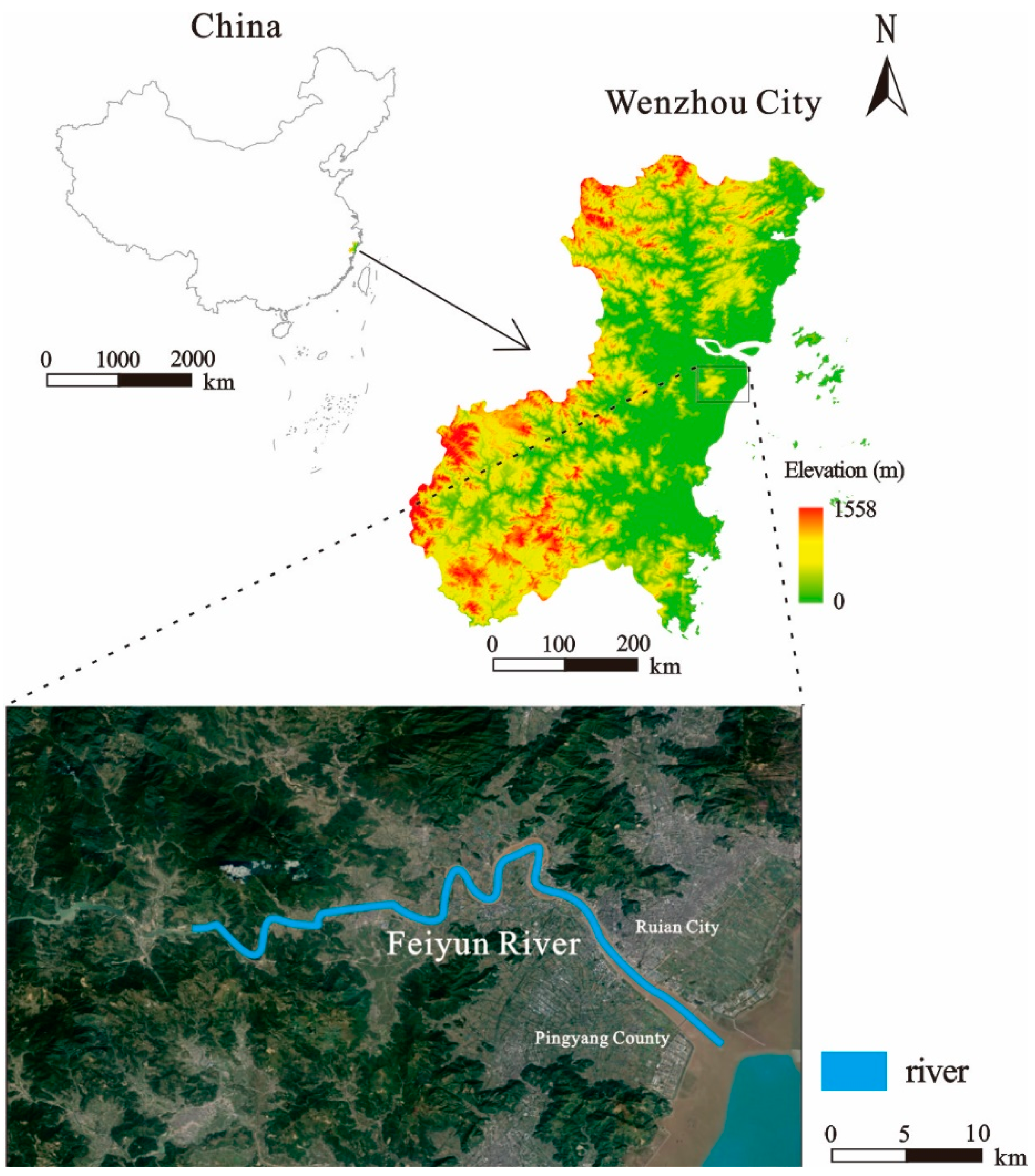

Figure 3.
The slope model used in this study: (a) the vegetation setting viewed from the front, (b) the vegetation setting viewed from the side, and (c) the schematic diagram showing the geometry characteristics of the slope model.
Figure 3.
The slope model used in this study: (a) the vegetation setting viewed from the front, (b) the vegetation setting viewed from the side, and (c) the schematic diagram showing the geometry characteristics of the slope model.
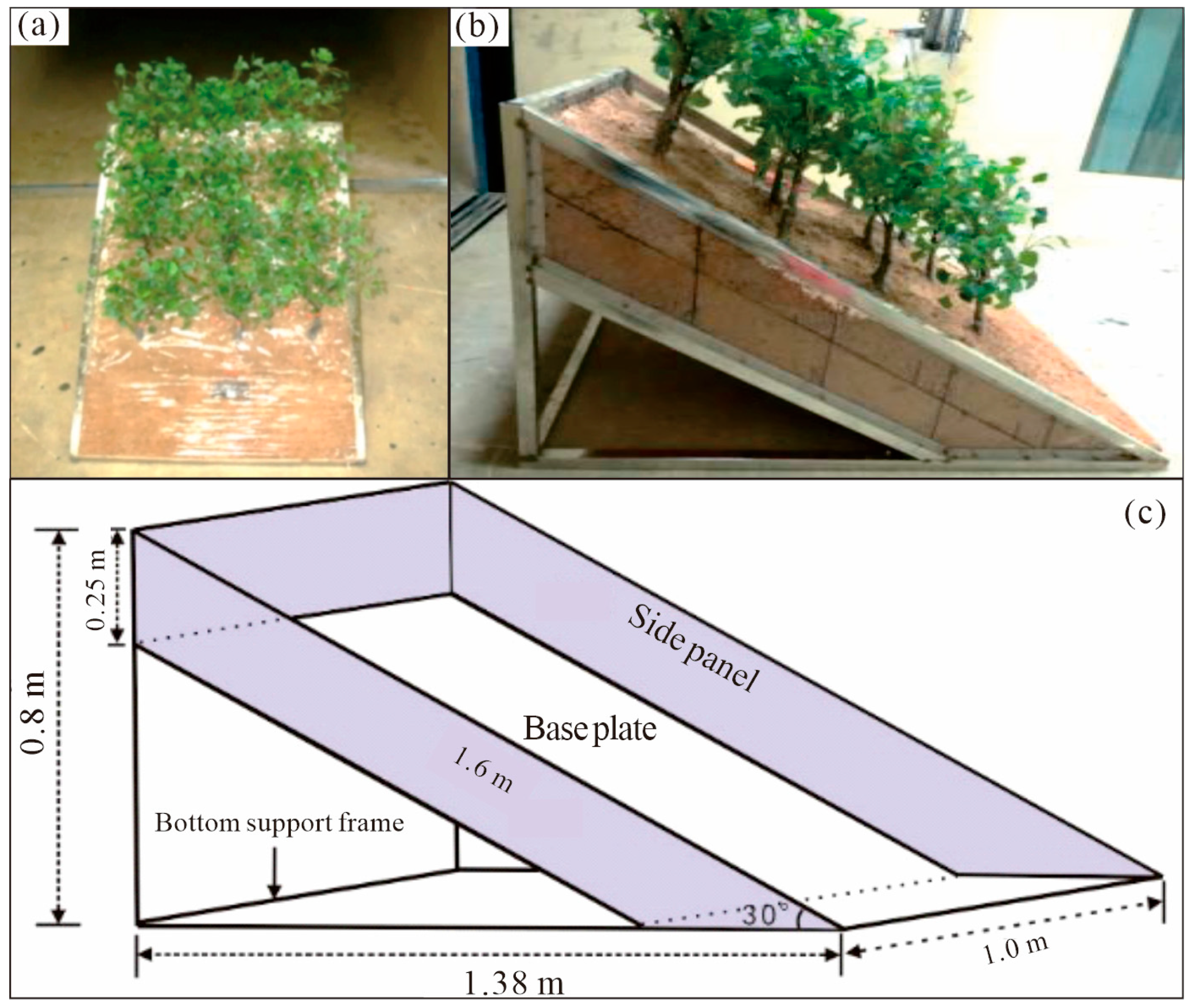
Figure 4.
(a) Setup of wind pressure monitoring point for the tree; (b) DTC initium pressure scanning data acquisition system.
Figure 4.
(a) Setup of wind pressure monitoring point for the tree; (b) DTC initium pressure scanning data acquisition system.
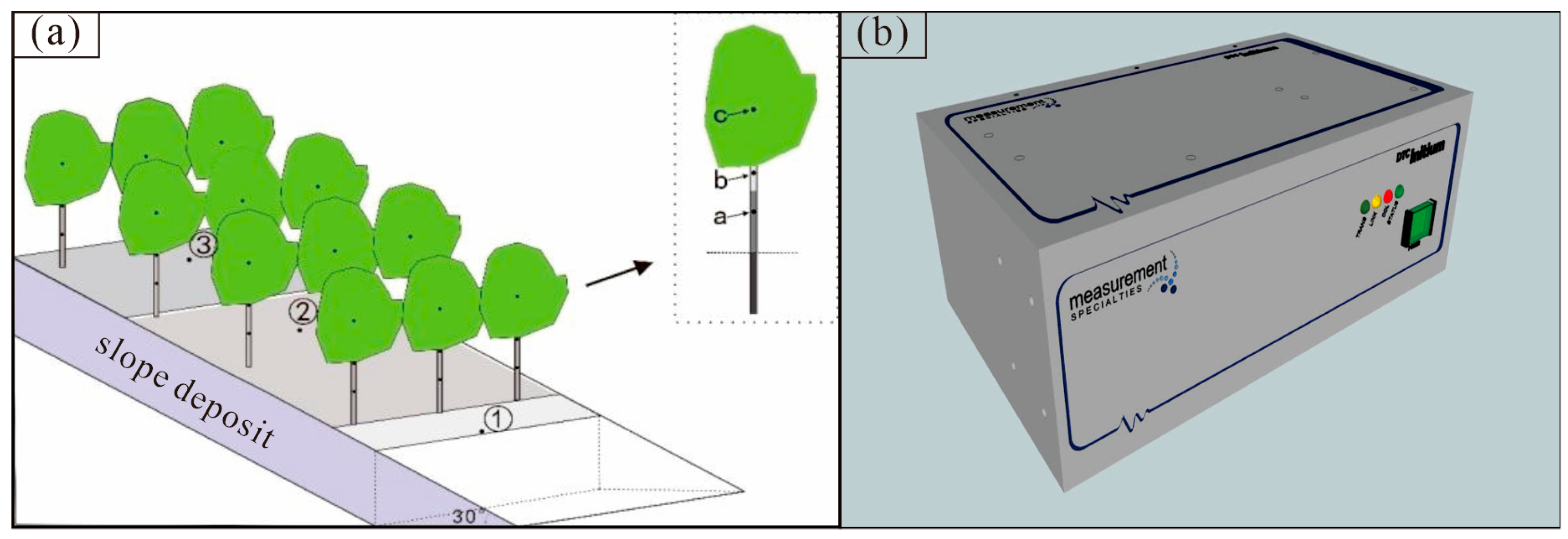
Figure 5.
(a) Schematic representation of the analytical profile, and (b) schematic diagram of slope wind load calculation partition simplification.
Figure 5.
(a) Schematic representation of the analytical profile, and (b) schematic diagram of slope wind load calculation partition simplification.
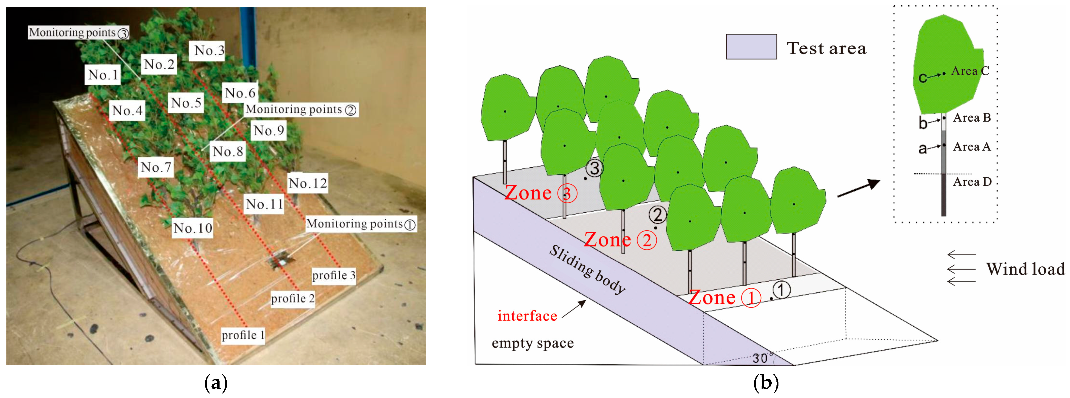
Figure 6.
Schematic diagram of the forces on the slope under wind load.
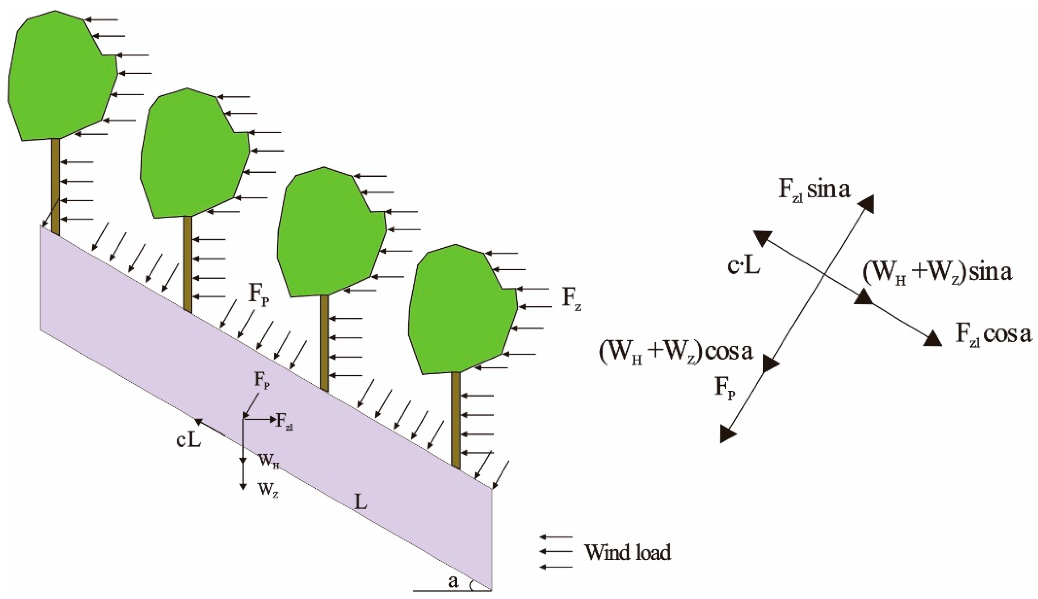
Figure 7.
Vegetation damage under different wind speeds: (a) 8.3 m/s; (b) 10.3 m/s; (c) 13.4 m/s; (d) 17 m/s.
Figure 7.
Vegetation damage under different wind speeds: (a) 8.3 m/s; (b) 10.3 m/s; (c) 13.4 m/s; (d) 17 m/s.

Figure 8.
Wind pressure variation for each tree on profile 1 at a wind speed of 8.3 m/s: (a) Tree #10; (b) Tree #7; (c) Tree #4; (d) Tree #1.
Figure 8.
Wind pressure variation for each tree on profile 1 at a wind speed of 8.3 m/s: (a) Tree #10; (b) Tree #7; (c) Tree #4; (d) Tree #1.
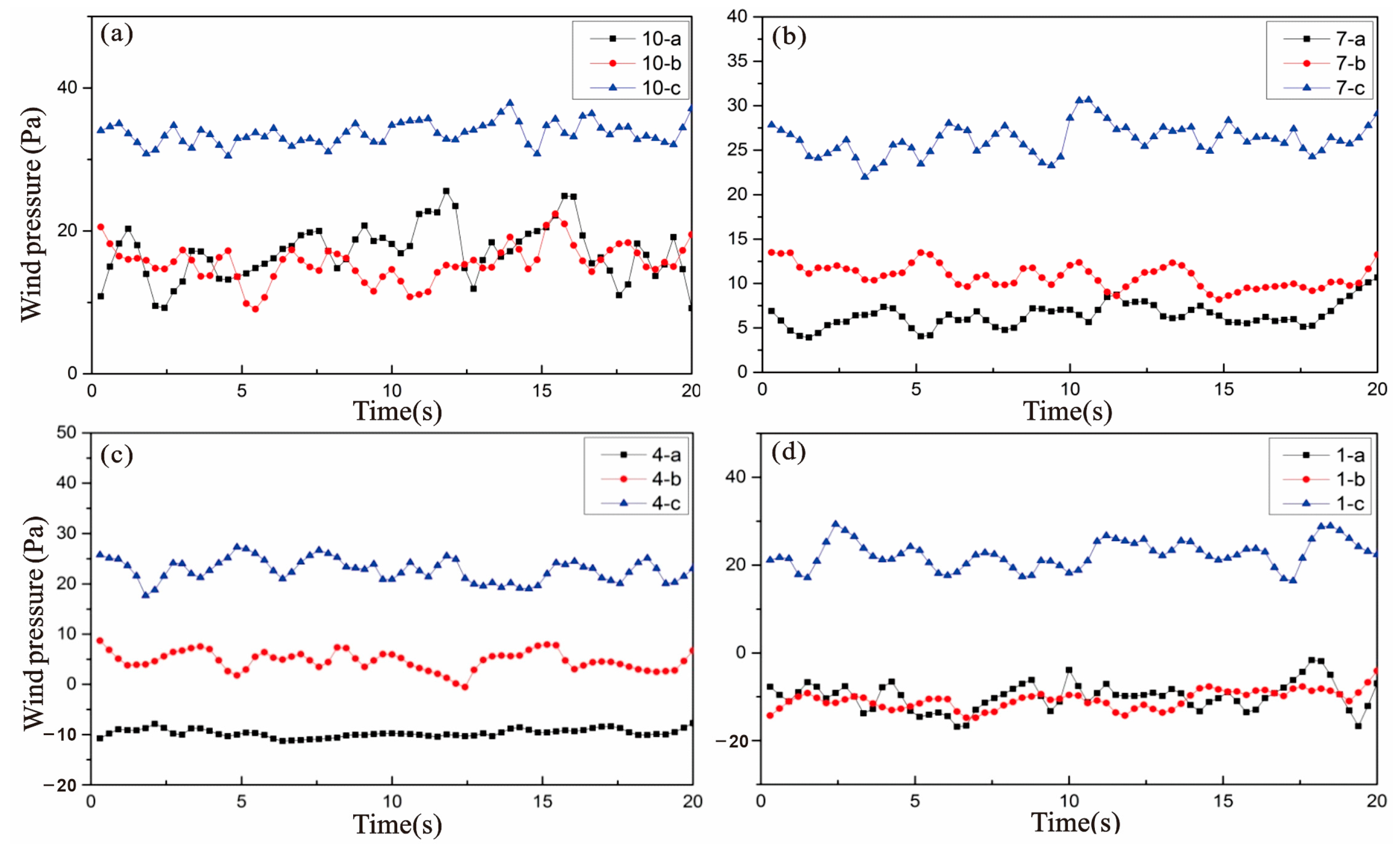
Figure 9.
Wind pressure variation for each tree on profile 2 at a wind speed of 8.3 m/s: (a) Tree #11; (b) Tree #8; (c) Tree #5; (d) Tree #2.
Figure 9.
Wind pressure variation for each tree on profile 2 at a wind speed of 8.3 m/s: (a) Tree #11; (b) Tree #8; (c) Tree #5; (d) Tree #2.
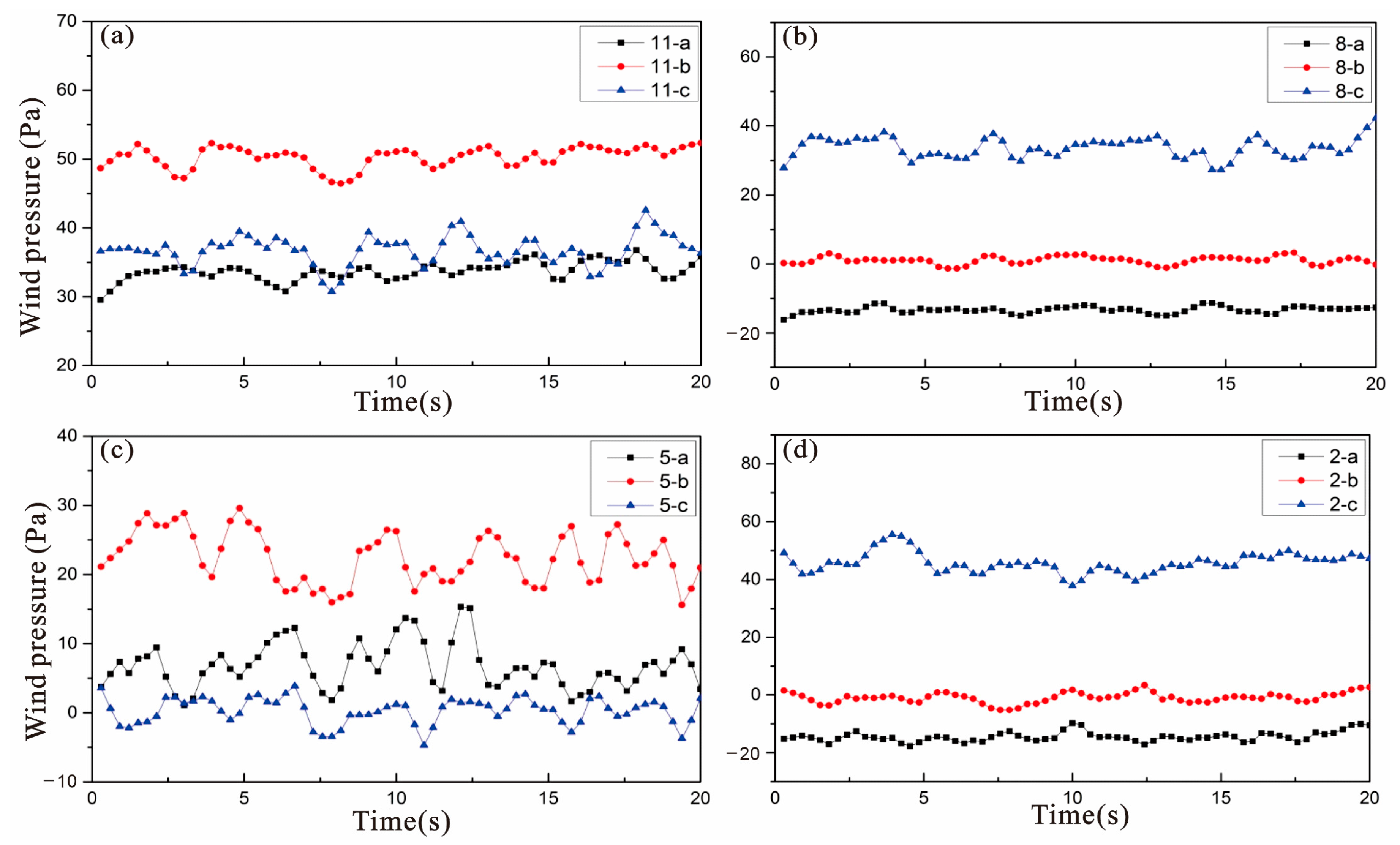
Figure 10.
Wind pressure variation for each tree on profile 3 at a wind speed of 8.3 m/s: (a) Tree #12; (b) Tree #9; (c) Tree #6; (d) Tree #3.
Figure 10.
Wind pressure variation for each tree on profile 3 at a wind speed of 8.3 m/s: (a) Tree #12; (b) Tree #9; (c) Tree #6; (d) Tree #3.
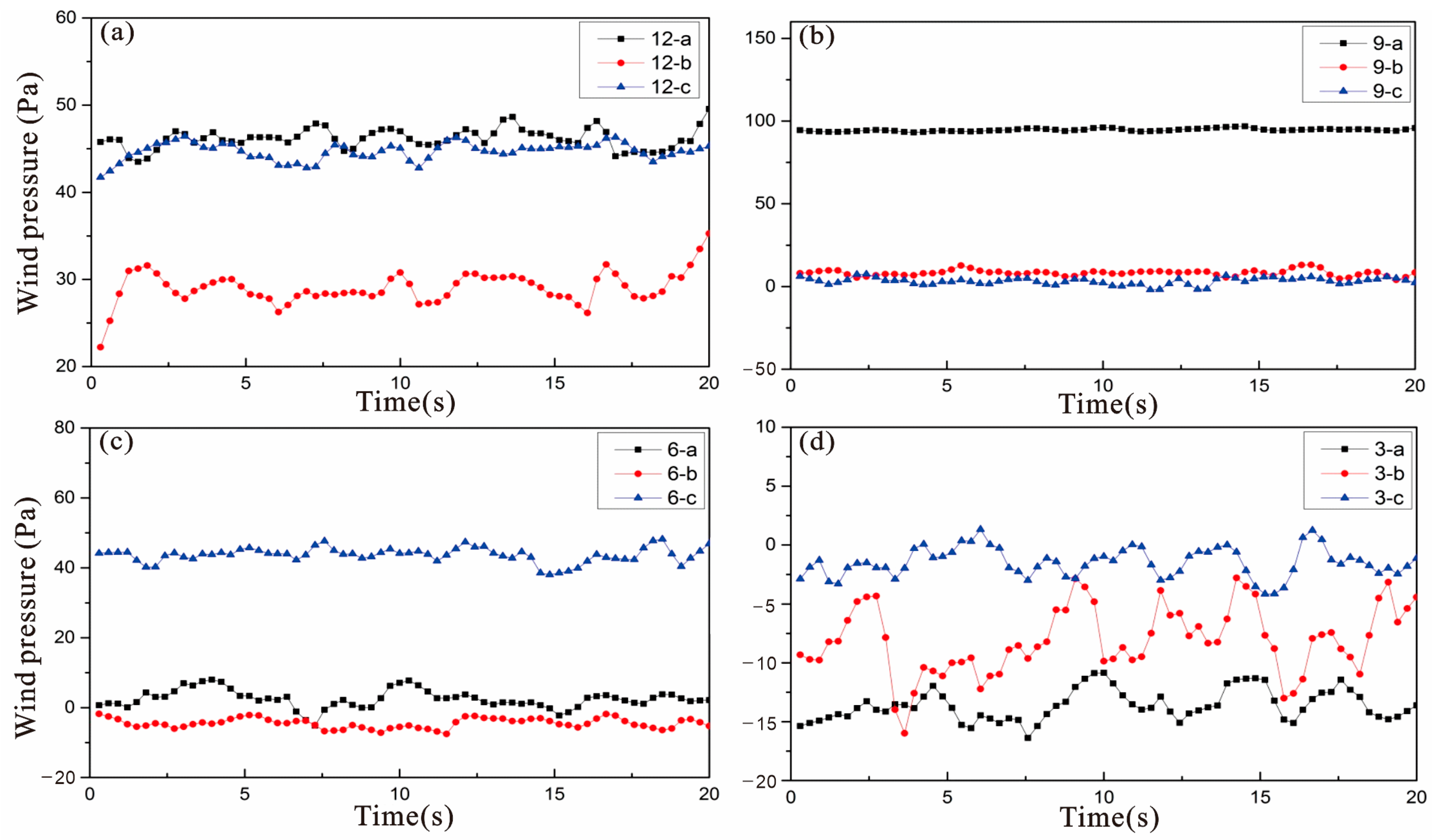
Figure 11.
Wind load values of each tree at different wind speeds: (a) wind speed of 8.3 m/s; (b) wind speed of 10.3 m/s; (c) wind speed of 13.4 m/s; and (d) wind speed of 17 m/s.
Figure 11.
Wind load values of each tree at different wind speeds: (a) wind speed of 8.3 m/s; (b) wind speed of 10.3 m/s; (c) wind speed of 13.4 m/s; and (d) wind speed of 17 m/s.

Figure 12.
Wind load curves for different areas on the slope at different wind speeds: (a) wind speed of 8.3 m/s; (b) wind speed of 10.3 m/s; (c) wind speed of 13.4 m/s; and (d) wind speed of 17 m/s.
Figure 12.
Wind load curves for different areas on the slope at different wind speeds: (a) wind speed of 8.3 m/s; (b) wind speed of 10.3 m/s; (c) wind speed of 13.4 m/s; and (d) wind speed of 17 m/s.

Figure 13.
(a) The residual sliding force of the slope under different states and (b) the calculated safety factor of the slope under different states.
Figure 13.
(a) The residual sliding force of the slope under different states and (b) the calculated safety factor of the slope under different states.

Table 1.
Geometric parameters of the slope prototype and the interior model.
| Type | Geometric Parameter | Vegetation Parameter | Physical and Mechanical Parameters | ||||||
|---|---|---|---|---|---|---|---|---|---|
| Parameter | Landslide Length | Landslide Width | Sliding Depth | Vegetation Height | Vegetation Root Depth | Density | Cohesion | Friction Angle | Moisture Content |
| prototype | 25 m | 16 m | 4 m | 9.5 m | 2.5 m | 1.8 g/cm3 | 30 kPa | 28° | 15% |
| model | 1.56 m | 1 m | 0.25 m | 0.6 m | 0.15 m | 1.8 g/cm3 | 2 kPa | 28° | 15% |
Disclaimer/Publisher’s Note: The statements, opinions and data contained in all publications are solely those of the individual author(s) and contributor(s) and not of MDPI and/or the editor(s). MDPI and/or the editor(s) disclaim responsibility for any injury to people or property resulting from any ideas, methods, instructions or products referred to in the content. |
© 2024 by the authors. Licensee MDPI, Basel, Switzerland. This article is an open access article distributed under the terms and conditions of the Creative Commons Attribution (CC BY) license (https://creativecommons.org/licenses/by/4.0/).
Share and Cite
MDPI and ACS Style
Guo, Z.; Liu, Y.; Zhang, T.; Zhang, J.; Wang, H.; He, J.; Li, G.; Tian, B. Revealing the Effect of Typhoons on the Stability of Residual Soil Slope by Wind Tunnel Test. Forests 2024, 15, 791. https://doi.org/10.3390/f15050791
AMA Style
Guo Z, Liu Y, Zhang T, Zhang J, Wang H, He J, Li G, Tian B. Revealing the Effect of Typhoons on the Stability of Residual Soil Slope by Wind Tunnel Test. Forests. 2024; 15(5):791. https://doi.org/10.3390/f15050791
Chicago/Turabian StyleGuo, Zizheng, Yuanbo Liu, Taili Zhang, Juehao Zhang, Haojie Wang, Jun He, Guangming Li, and Bixia Tian. 2024. "Revealing the Effect of Typhoons on the Stability of Residual Soil Slope by Wind Tunnel Test" Forests 15, no. 5: 791. https://doi.org/10.3390/f15050791
Note that from the first issue of 2016, this journal uses article numbers instead of page numbers. See further details here.