Article

The Effect of Urban Green Spaces on the Urban Thermal Environment and Its Seasonal Variations

1
Northeast Institute of Geography and Agroecology, Chinese Academy of Sciences, Changchun 130102, China
2
University of Chinese Academy of Sciences, No. 19A Yuquan Road, Beijing 100049, China
3
College of Earth Science, Jilin University, Changchun 130061, China
*
Author to whom correspondence should be addressed.
Forests 2017, 8(5), 153; https://doi.org/10.3390/f8050153
Submission received: 26 January 2017 / Revised: 19 April 2017 / Accepted: 28 April 2017 / Published: 2 May 2017

Abstract

:
Urban green spaces have been shown to decrease land surface temperature (LST) significantly. However, few studies have explored the relationships between urban green spaces and LST across different seasons at different spatial scales. In this study, using Changchun, China as a case study, landscape ecology and comparative approaches were employed quantitatively to investigate the effects of the composition and configuration of urban green spaces on the urban thermal environments. LST maps were retrieved from Landsat 8 Thermal Infrared Sensor (TIRS) data acquired on four dates that represented four different seasons, and detailed information of urban green spaces was extracted from high resolution imagery GF-1. Normalized differential vegetation index (NDVI) and six landscape metrics at patch, class, and landscape level were used to characterize the spatial patterns of urban green spaces. The results showed that urban green spaces did have significant cooling effects in all seasons, except for winter, but the effects varied considerably across the different seasons and green types, and seemed to depend on the NDVI and size of urban green spaces. Compared to shape metrics, the negative relationships between the LST and the area and the NDVI of urban green spaces were more significant. Both the composition and configuration of urban green spaces can affect the distribution of LST. Based on findings with one city, given a fixed area of urban green spaces, the number of green patches can positively or negatively affect the LST, depending on if the number is larger than a threshold or not, and the threshold varies according to the given area. These findings provide new perspectives, and further research is also suggested, to generate a better understanding of how urban green spaces affect the urban thermal environment.

1. Introduction

According to the United Nations, over half of the world’s population (54%) lived in urban areas in 2014, and this number is projected to increase to 66% by 2050 as a result of rapid urbanization [1]. Therefore, more people will suffer from urban heat island (UHI) effects, which are caused by dramatic changes in land use and land cover, energy use, and air-pollutant emissions [2,3,4]. Intensive heat can cause many negative effects, including significant health and well-being problems for urban inhabitants over the long term, and especially for the elderly [5,6,7]. There is no doubt that understanding how to mitigate its negative impacts is one of the most important research issues for urban ecology and urban climatology.
Urban green spaces, such as open parks, forests, and grasslands, have been increasingly recognized as key components of urban planning [8,9,10,11]. Urban green spaces have been shown to form cool islands and improve outdoor thermal comfort throughout warm seasons, as well as significantly reduce environmental stress produced by heat island [12,13]. They can also provide critical ecosystem services that could improve residents’ health and wellbeing [13,14,15]. Urban green spaces can cool climates through two major processes: shading and by providing higher evapotranspiration [8,16,17]. As a result, over the past two decades, many studies have focused on understanding the effects of urban green spaces on the urban thermal environment [11,12,17,18,19,20,21].
With the development of remote sensing technology, thermal infrared remote sensing and high resolution remote sensing images have been extensively utilized in urban climate and environment studies [22,23,24]. Land surface temperature (LST) is a universal and important parameter for characterizing the urban thermal environment [25,26]. LST modulates the underlying urban air temperature and is a primary factor for determining surface radiation and human comfort [27,28]. At present, among the numerous data sources that are available, the Landsat series is most popular for retrieving LST for urban studies, as it has the advantage of higher spatial resolution (TM 120 m/ETM+ 60 m/Thermal Infrared Sensor (TIRS) resampled to 30 m) than Moderate Resolution Imaging Spectroradiometer (MODIS) and Advanced Very High Resolution Radiometer (AVHRR) [29,30,31]. Advances in the datasets used to characterize land use allow researchers to better understand urban spatial patterns. Very high spatial resolution images, such as IKONOS and Quickbird, combined with thermal infrared images are widely used in urban ecology studies, making it possible to establish more accurate relationships between one single object and LST in finer scales [32,33,34].
Moreover, the landscape ecology approach has been used to explore the relationships between urban green space patterns and the urban thermal environment [32,35,36]. Many studies have determined that the size, shape, composition, spatial characteristics, and configuration of urban green patches have significant effects on the distribution of LST [37,38]. To characterize urban green space landscape patterns, two kinds of landscape metrics have been popularly used by scientists: landscape composition and landscape configuration [39,40]. Landscape composition metrics usually indicate the amount of area and type of land use, but do not provide any spatial information. In contrast, landscape configuration considers the geographic features of each land use type. Though increasing urban green spaces is an important strategy to mitigate UHI effects, metropolitan areas usually lack sufficient public spaces to create all of the urban green spaces that they need. Therefore, efficiently arranging urban green spaces within a fixed amount of available space has become increasingly more important because landscape configuration also affects radiative fluxes and energy flows [41]. Many metrics have been developed to measure the effects of landscape patterns, such as area metrics, perimeter-area ratio, landscape shape index, and aggregation metrics [29,35,42]. FRAGSTATS software (University of Massachusetts, Amherst, MA, USA) is widely used to calculate these metrics [43].
Urban green spaces are diverse, with varying species compositions, functions, management policies, and many other aspects. Existing studies are essential for urban planning and sustainable development of urban environment, but more studies are needed within cold regions in particular to enrich the theory and the number of case studies available. Most studies explore the effect of urban green spaces on the urban environment in summer, while neglecting to study its effects during other seasons. The growth conditions of green spaces differ significantly in different seasons. As such, year-round study may provide a more comprehensive understanding of the mechanisms that affect how urban green spaces mitigate UHI effects. In addition, when using landscape approaches, often only one metric level is considered, especially at patch level or landscape level. The class level, however, is also important for understanding the effect of urban green spaces because different types have different contributions. Comparative approaches are needed to investigate the effect of urban green spaces at multiple different spatial scales rather than just one single scale which is the spatial resolution of the imagery data.
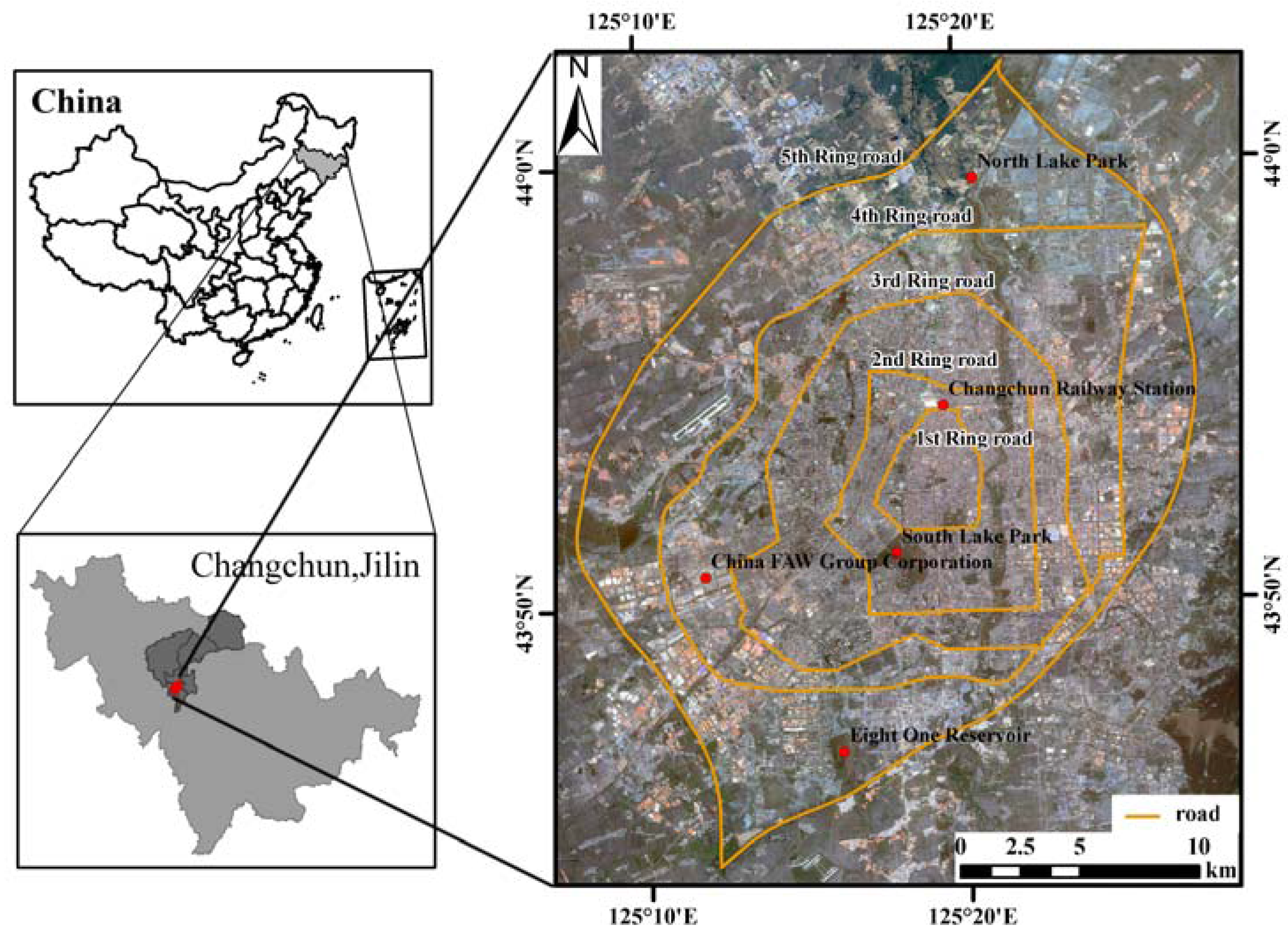
This paper aims to identify appropriate metrics that effectively describe the features of urban green spaces in order to investigate how different green spaces and their spatial configurations affect the urban thermal environments at different spatial scales across different seasons and to establish quantitative relationships between these aspects. To achieve our goals, very high spatial resolution imagery GF-1 (2-m spatial resolution) was utilized to obtain detailed information of urban green spaces, and Landsat 8 TIRS (30-m spatial resolution) was chosen to provide data on the urban thermal environment in spring, summer, autumn, and winter in Changchun, China.

2. Materials and Methods

2.1. Study Area

Changchun city (125°06′–125°36′ E, 43°43′–44°04′ N) (Figure 1), which is the capital of Jilin province, China, is located in the northern hemisphere mid-latitude regions, with an urban population of 3.65 million (2014). The city serves as the financial center and cultural heart of the province. In the past 30 years, Changchun has been undergoing an accelerated process of urbanization, with the urban built-up area having increased from 138.4 km2 in 1984 to 557.9 km2 in 2014 [44]. According to the National Economy and Society statistical bulletin of Changchun in 2014, the proportion of urban green area in the Changchun built-up area is approximately 36.5%, and the per capita green area is about 11.6 m2.
The region is characterized by a sub-humid continental climate, four seasons with a long, cold winter and a short, hot summer. According to meteorological records of 1951–2014, the annual precipitation of Changchun is 561.6 mm and the annual average temperature is 5.5 °C, with a hot July (23.1 °C) and a cold December (−12.3 °C). The annual average air temperature has increased by 1.86 °C during last 60 years from 1951 to 2011 [38]. As a result of urbanization, the average urban air temperature is about 0.1–0.5 °C higher than that of surrounding rural areas based on the local meteorological data.
There are few studies using Landsat 8 data and very high resolution images to estimate the relationships between urban green spaces and thermal environments in the cold temperate zone. This study may help to provide new insights for UHI mitigation and urban planning.

2.2. Urban Green Spaces Extraction

Detailed information of urban green spaces was derived from a GF-1 image acquired on 22 June 2015 that was provided by the China Center for Resources Satellite Data and Application (CRESDA). GF-1 is equipped with two multispectral scanners with 2 m resolution panchromatic and 8 m resolution multispectral, and 4 multispectral scanners with 16 m resolution. Satellite engineering made a breakthrough in optical remote sensing technology by integrating high space resolution, multispectrum, and high time resolution. The multispectural and panchromatic images were first fused to produce a four-band pan multispectral image with a resolution of 2 m. The images fusion was performed in ENVI 5.3. First, RPC Orthorectification Workflow was applied to the multispectral (4 m) and panchromatic (2 m) images, then Image Registration Workflow was used to perform image registration. Finally, the NNDiffuse Pan Sharpening method was used to fuse images. The urban green spaces were manually classified into six types based on their locations and services, as defined in Table 1. Visual interpretation was used to extract information about the green spaces, including the boundary and type of each patch, according to location, size, shape, and spatial relationships with neighbors. In addition, Google Earth maps with higher spatial resolution were combined to identify the type of patch. In our case, the minimum patch size is 200 m2. Fieldwork conducted during August 2015 resulted in the acquisition of 96 ground references for accuracy assessment. Overall, the total accuracy of the derived urban green map achieved 92.1%.

2.3. Land Surface Temperature

The successful launch of Landsat 8 on 11 February 2013 with the most advanced Thermal Infrared Sensor (TIRS) is anticipated to extend the 40-year Landsat record for at least another 5 years [31]. A series of Landsat 8 TIRS images with 100 m resolution (resampled to 30 m) acquired on 10 April, 22 July, 3 October, and 22 December 2014 from the USGS (United States Geological Survey) website, which represented spring, summer, autumn, and winter, respectively, were utilized to derive LST to characterize the urban thermal environment. There was almost no cloud cover in the study area on the dates of acquisition. A mono-window algorithm (MWA) presented by Qin et al. [45] was used to map LST, with only three parameters required: emissivity, transmittance, and effective mean atmospheric temperature without the use of atmospheric profiles. The basic form can be written as:
Ts = [a(1 − CD) + (b(1 − CD) + C + D)TiDTa]/C
where T s is LST, T i is brightness temperature of TIRS bands i, and T a is the effective mean atmospheric temperature. The value of constants a and b are −67.366351 and 0.458606, respectively, and C and D are defined as follows:
C = ετD = (1 − τ)[1 + (1 − ε)τ]
where ε and τ are land surface emissivity (LSE) of band i and atmospheric transmittance of band i, respectively. In this study, Landsat 8 TIRS band 10 takes the place of TM band 6 in MWA. The calculations for T i , ε , τ , and T a are detailed in previous studies [46,47,48,49,50].
Air temperature collected from 19 local meteorological stations located in the study area were used to validate the precision of the retrieved LST from Landsat images. The acquisition time of the two remote sensing images on 31 July 2014 was 10:21 a.m. However, measurements of the ground-truth LST were limited by the difficulty of finding a homogeneous region as large as the satellite pixel size. As a result, the average retrieved LST of the 9 × 9 pixels near the meteorological station was compared to the mean air temperature acquired on 10:00 a.m. and 11:00 a.m.

2.4. Characterizing the Urban Green Spaces

Landscape ecology, if not ecology in general, is largely founded on the notion that environmental patterns strongly influence ecological processes [51]. Landscape metrics are versatile and widely used to measure landscape patterns [40,43]. Six landscape metrics were chosen to quantitatively characterize the urban green spaces based on the following principles: (1) easily calculated; (2) scientific and practical importance [52,53]. The patch level metrics were patch area (PA), patch perimeter (PERIM), perimeter-area ratio (PARA), shape index (SHAPE), and class level metrics, including total area (TA). The landscape level metrics were: total area (TA) and number of patches (NP). All of these metrics and their descriptions are listed in Table 2.
As composition metrics, PA and TA are perhaps the most important and useful pieces of information regarding the landscape because they are used as the basis for many of the patch, class, and landscape indices [43]. PARA and SHAPE are shape metrics that quantify landscape configuration in terms of the complexity of patch shape at different levels. For example, a square patch is SHAPE = 1, and a higher SHAPE value indicates higher shape complexity. NP is an aggregation metric that refers to the tendency of patch types to be spatially aggregated. This property is also often referred to as landscape texture. These metrics characterize the composition and configuration information of urban green spaces. In this study, all the metrics were calculated by FRAGSTATS, which is a spatial pattern analysis program for quantifying the structure of landscapes.
For landscape level metrics, in order to build quantitative relationships between urban green spaces and LST at multiple resolutions, two spatial scales were selected: 1 km × 1 km and 0.5 km × 0.5 km. Fishnet in ArcGIS 10.2 (ESRI, Redlands, CA, USA) was used to create these grids, and there were 577 and 2206 sections for the scales of 1 km × 1 km and 0.5 km × 0.5 km, respectively. Each section is treated as a single landscape, and landscape metrics and LST were calculated for every grid. As a result, the spatial pattern of the landscape level metrics could be shown as theme maps to provide more distinct information compared to conventional tables.
In addition, at the patch and class level, NDVI (normalized difference vegetation index) was used to describe the amount of urban green spaces and growth status. High values of NDVI tend to correlate with more vegetation and good “condition” of vegetation. NDVI is defined as follows:
NDVI = N I R R N I R + R
where NIR is band 5 and R is band 4 for Landsat 8.

2.5. Statistical and Comparative Analysis

Existing research studies on relationships between urban green spaces and LST have used both qualitative and quantitative models [9,50]. In this study, all statistical analyses were conducted with SPSS 19.0. First, one-way analysis of variance (ANOVA) was conducted to examine whether the landscape metrics calculated from the three levels, the LST and NDVI of each patch, class, and landscape were significantly different and redundant. Then, bivariate correlations were performed to analyze the relationships between these metrics and corresponding LST. At the patch level, as the distribution of the area of the urban green space patches is not normal, Spearman’s rho correlation coefficients were chosen to explore the relationships between the mean LST for each patch, landscape metrics, and NDVI on 31 July 2014. The area of a single TIRS image pixel was 900 m2 (0.09 ha). In cases where the PA is not as large as the area depicted in the pixel, it is difficult to obtain accurate LST for each patch. For this reason, in our case, only the green space patches with areas larger than 0.36 ha (≥4 TIRS pixels) were selected to perform bivariate correlations, and these were classified into six classes depending on the patch size. At the landscape level, eight regression models were performed using the metrics and mean LST of each grid across the four seasons at different scales to identify the metrics most relevant to the LST.

3. Results

3.1. Spatial Pattern of Urban Green Spaces

The spatial distribution of urban green spaces in Changchun is shown in Figure 2. The total area of green space is distributed across 115.84 km2 with 8287 patches, and all are located within the 5th Ring Road. As shown in Table 3, Attached Green Spaces (AGS) patches were observed to have the smallest mean area, while Park Green Spaces (PGS) patches had the largest. However, AGS was observed to have the largest total area followed by Ecological Green Spaces (EGS), Road Green Spaces (RGS), PGS, Other Green Spaces (OGS), and Productive Plantation Green Spaces (PPGS). Table 3 provides detailed statistical information about the urban green spaces.

3.2. Spatial Pattern of LST

The LST distribution in Figure 3 shows the contrasts between surface temperature for different dates. The results showed that the average satellite-based LST was approximately 4.6 °C higher than the average air temperature, which was reasonable for the hot summer. Hence, the retrieved LST by the same algorithm in other seasons can also reflect the urban thermal environment. There were remarkable seasonal variations in LST. The average LST of the study area was 20.97 °C, 35.57 °C, 16.35 °C, and −14.56 °C in spring, summer, autumn, and winter, respectively. In spring, summer, and autumn, lower surface temperatures were found in urban green spaces. In contrast, in the winter, this phenomenon was not as apparent. The largest range of LST was found in the summer, representing the largest temperature contrast of all of the seasons. Detailed information of the LST in the study area for the four seasons is shown in Table 4.

3.3. The Effect of Urban Green Spaces on Thermal Environment

3.3.1. Patch Level

As an indicator of the status of vegetation, Table 5 shows that the mean NDVI of each patch was significantly negatively correlated to LST among all the classes, indicating that higher NDVI values can lead to lower LST. When the area of green space patch is between 1.44 and 5.76 ha, the negative relationship between LST and PA is significant and much stronger than for the other classes, indicating that in this area range increasing the PA can lower LST. While in other area ranges, it appears that the PA has little influence on its own LST. For other landscape metrics, the relationships between LST and PERIM, PARA, and SHAPE were very weak. There are two exceptions. When the PA is larger than 15.2 ha, the negative relationships between LST and PERIM, and SHAPE were significant and stronger. It appears that the SHAPE metric begins to have influence on the mean LST of green space patches in this area range. These relationships suggest that compared to NDVI, landscape metrics including PERIM, PARA, and SHAPE have little influence on the mean LST of green space patches. When the PA of one patch is less than 1.44 ha or larger than 5.76 ha, it has little effect on its own mean LST.
A summary of the stepwise regression model is shown in Table 6. The results showed that the standardized coefficients of variables differed greatly and all variables except for PA were included in the best fit model, indicating that the PA of each patch had little influence on its own mean LST. Compared to other patch-level metrics, NDVI is the most important variable in determining the LST. Different from other variables, a positive relationship was detected between PARA and LST.

3.3.2. Class Level

The average LST and standard deviation of each green type were lower than the mean LST of the city as a whole in all dates except for 22 December, as shown in Table 4 and Table 7. The NDVI for each green type was greater than the average values of the overall area with 0.12, 0.42, 0.25, and 0.05 for 10 April, 31 July, 3 October, and 22 December, respectively. For seasonal variations, the correlation coefficients between the mean LST and NDVI of the six green spaces classes were −0.42, −0.94 (0.01 level, one-tailed), −0.93 (0.01 level, one-tailed), and −0.74 (0.05 level, one-tailed) for dates 10 April, 31 July, 3 October, and 22 December, respectively. PGS had the lowest mean LST and highest NDVI across all seasons except winter, while AGS and RGS had a high mean LST and a low NDVI relative to that of PGS.

3.3.3. Landscape Level

The temperature difference (TD) and NDVI difference between the whole study area and urban green spaces across the four dates are shown in Figure 4. In the winter, there was almost no TD between urban green spaces and the entire study area. The NDVI values of green spaces were lower than those of the study area across all seasons with the greatest difference in summer and the least in winter.
The spatial distributions of landscape-level metrics TA and NP are shown in Figure 5. Higher vegetation cover is located in the northeast and southeast part of study area where there are several big parks or lots of AGS patches in high density. The number of patches (NP) is high within the 4th Ring Road because there are many small AGS patches located in the oldest parts of the city. The spatial distributions of the two metrics suggests there is no obvious relationship between them.
Further quantitative regression models were established to explore the relationships between the landscape-level metrics and LST at 0.5 km × 0.5 km and 1 km × 1 km scales. Two-dimensional scatter plots are shown in Figure 6 and Figure 7. Negative linear relationships between LST and TA were found on all dates except for 22 December at the two different spatial scales. For season variations, negative relationships were strongest in summer followed by autumn and spring, and the relationships in winter were not significant. For spatial scale differences, compared to 0.5 km × 0.5 km, the negative relationships were stronger for the 1 km × 1 km scales across all the seasons. On 31 July at the 0.5 km × 0.5 km scale, a 1 ha increase in TA can result in approximately a 0.34 °C decrease in temperature. In other words, a 10% increase in TA can lead to a 0.85 °C decrease in temperature on this spatial scale. While on the same date at a 1 km × 1 km scale, a 10% increase in TA can lead to a 1.2 °C decrease in temperature, according to the statistical analysis. In other words, with an increase in TA, urban green spaces can result in a temperature decrease, but the cooling effect varies greatly at different seasons and spatial scales.
Three-dimensional images of TA (ha), NP, and LST across different seasons at different spatial scales were generated to explore the effect of configuration of urban green spaces on their cooling intensity. For the same area of urban green spaces, it appears that their spatial configurations can change significantly. For example, the number of patches and their locations play an important role in decreasing LST. For urban green space planning, the configuration cannot be ignored. In this study, the NP in particular spatial scales was chosen as the indicator to characterize the information for the configuration.
Figure 8 shows the 3-D images at the 0.5 km × 0.5 km scale. On 10 April, when the TA is the same, with the increase of NP, the LST has a negative trend. On 31 July, when the TA is less than 5 ha, the NP has little influence on LST. When TA is between 5 and 15 ha, an increase of NP can lead to lower LST. When TA is larger than 15 ha at this scale, NP is no longer the key factor in determining LST. On 3 October, when TA is less than 10 ha, NP has a negative relationship with LST. However, when TA is larger than 10 ha, the effect of NP on LST is not significant. On 22 December, because the urban green spaces have little influence on LST, their configurations also have little impact on LST.
Figure 9 shows the 3-D images at the 1 km × 1 km scale. On 10 April, with an increase of NP, the LST tends to have lower values. On 31 July, when the proportion of TA is less than 20%, regardless of NP, the LST is relatively high. When the proportion of TA is between 20% and 40%, at the beginning, with an increase of NP, the LST increases simultaneously. However, when NP is larger than 40, the LST decreases. When TA is larger than 40%, less NP can have a better cooling effect. On 3 October, when the percentage of TA is less than 20%, if NP is smaller than 50, the NP has little influence on LST. However, NP can result in a lower LST when it is larger than 50. A very interesting phenomenon is that with the increase of TA, the threshold value of NP can lead to lower LST decreases. For example, when the TA is between 30 and 40 ha, the threshold of NP is approximately 30. In contrast, when the TA is between 50 and 60 ha, the threshold of NP is approximately 10. However, when the NP is larger than the threshold value, the increase of NP has little effect on LST. These results indicate that when the TA is larger in this spatial scale, less NP may generate a better cooling effect. Compared to the 0.5 km × 0.5 km scale, on 22 December, with the increase of NP, the LST had an increasing trend at 1 km × 1 km scale.

4. Discussion

Representative landscape metrics at patch, class, and landscape level and quantitative statistical analysis were utilized to explore the effect of urban green spaces on the urban thermal environment. The results demonstrated that not only the composition of urban green spaces but also their configuration can significantly affect the distribution of the LST. The effect, however, varies greatly across different seasons depending considerably on the size and shape of urban green spaces, the status of vegetation, the analysis spatial scales, and seasonal radiation conditions. The results were consistent with many other previous studies, which demonstrated negative correlations between LST and urban green spaces [3,19,54].

4.1. Implications for Methodology

First, comparative approaches with an additional cold zone case study were utilized in this study to investigate the relationship between urban green spaces and the urban thermal environment. Comparative approaches included a selection of landscape metrics at three levels, patch, class, and landscape level. The four dates representing spring, summer, autumn, and winter were chosen to explore seasonal variations; two spatial scales, 0.5 km × 0.5 km and 1 km × 1 km, were selected to study the relationship changes across scales. These helped generalize a more thorough scientific understanding of the effects of urban green spaces on LST.
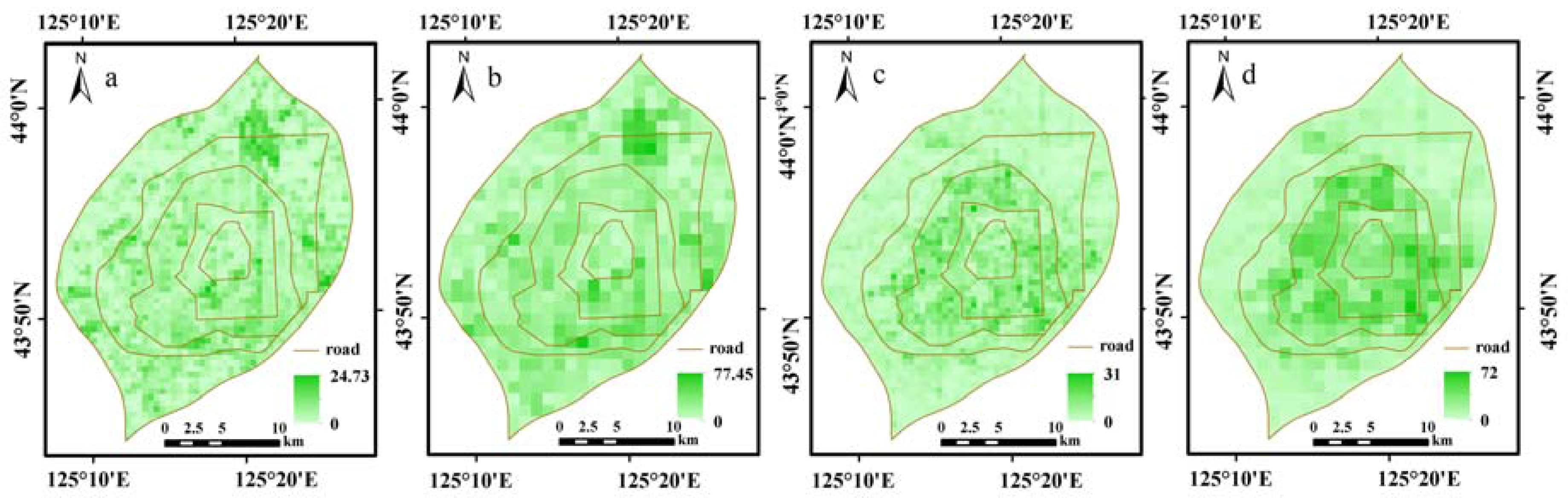
Second, we propose that spatialization is an important part of landscape metrics. Traditionally, the result of landscape metrics calculated by metrics software, such as FRAGSTATS, is often shown in tables. In this study, with the help of ArcGIS 10.2, 2206 and 577 grids were created in the study area at the scale of 0.5 km × 0.5 km and 1 km × 1 km, respectively. Each grid was considered as a whole landscape, and landscape-level metrics were calculated for each grid. As a result, the spatial information of the metrics were presented as maps in order to show the distribution of metrics in a more explicit way.

4.2. Theoretical Implications

In this study, landscape metrics and NDVI were used to characterize the composition features of urban green spaces.
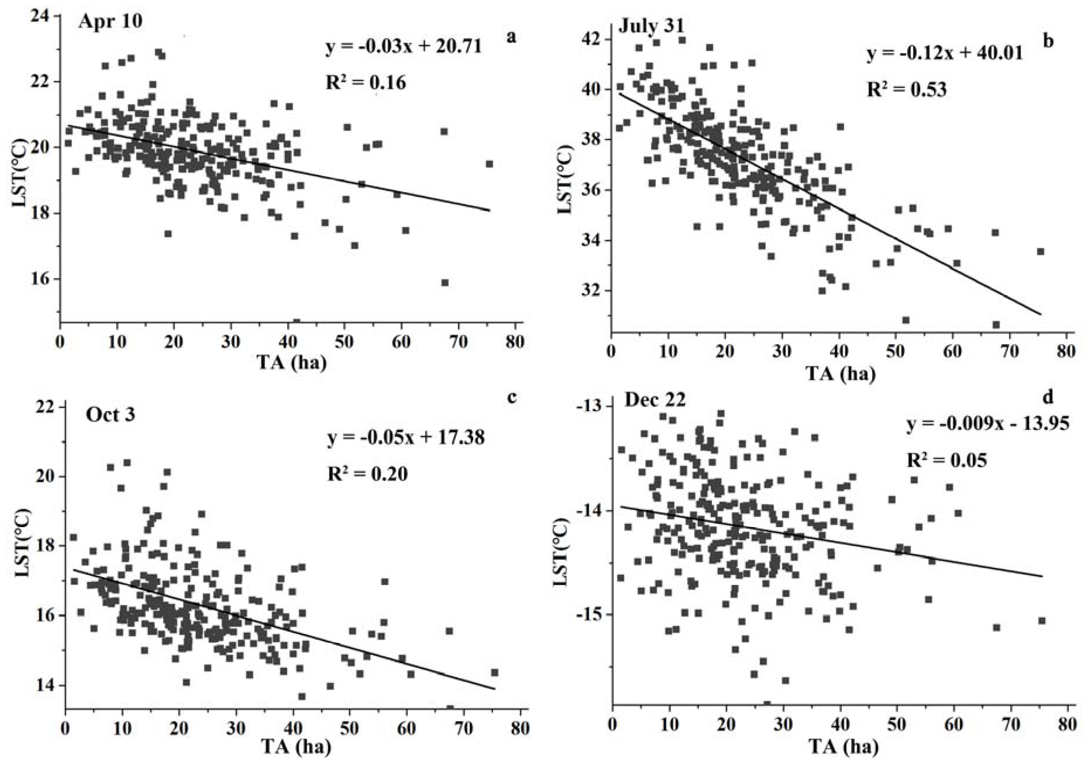
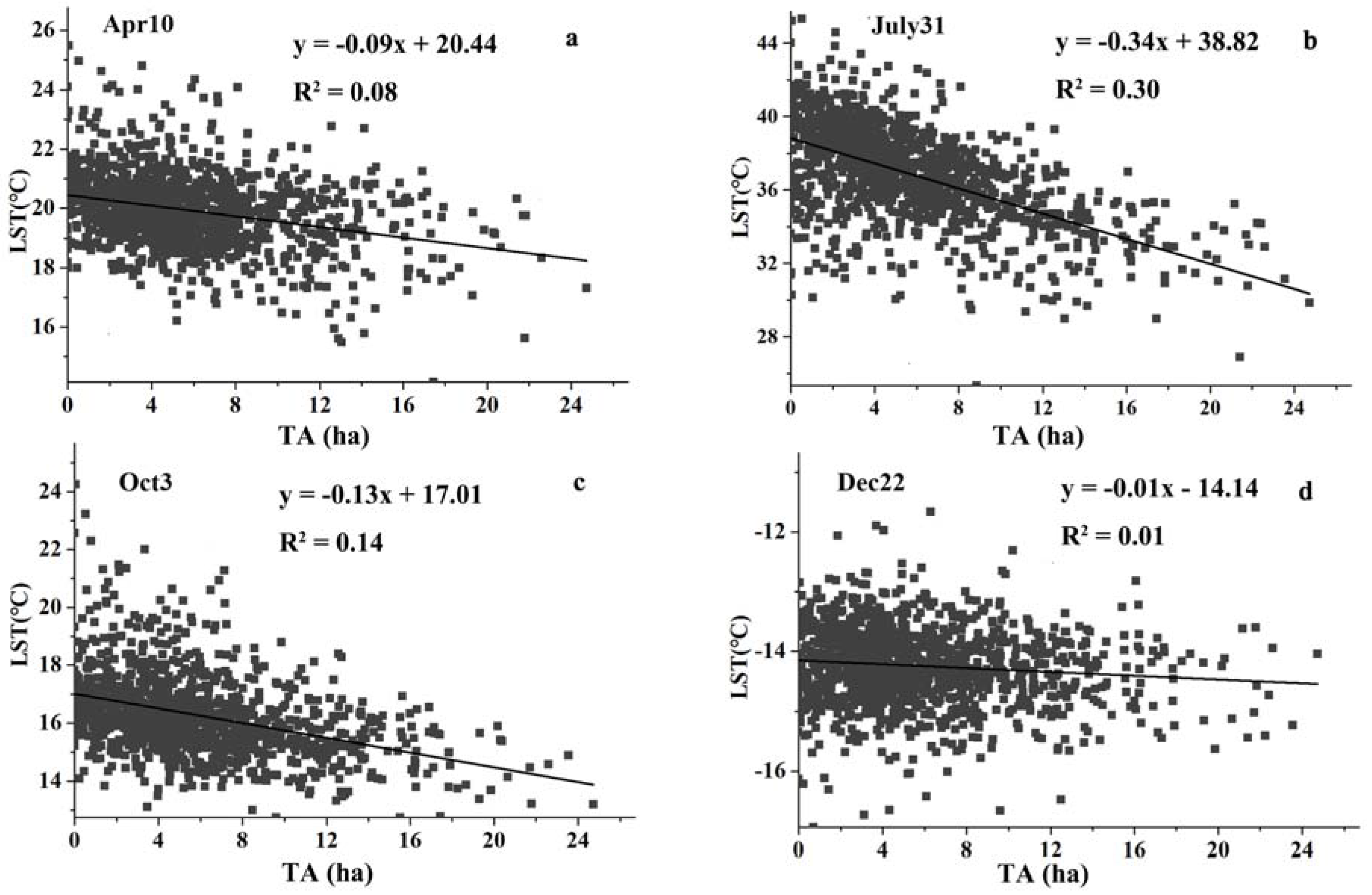
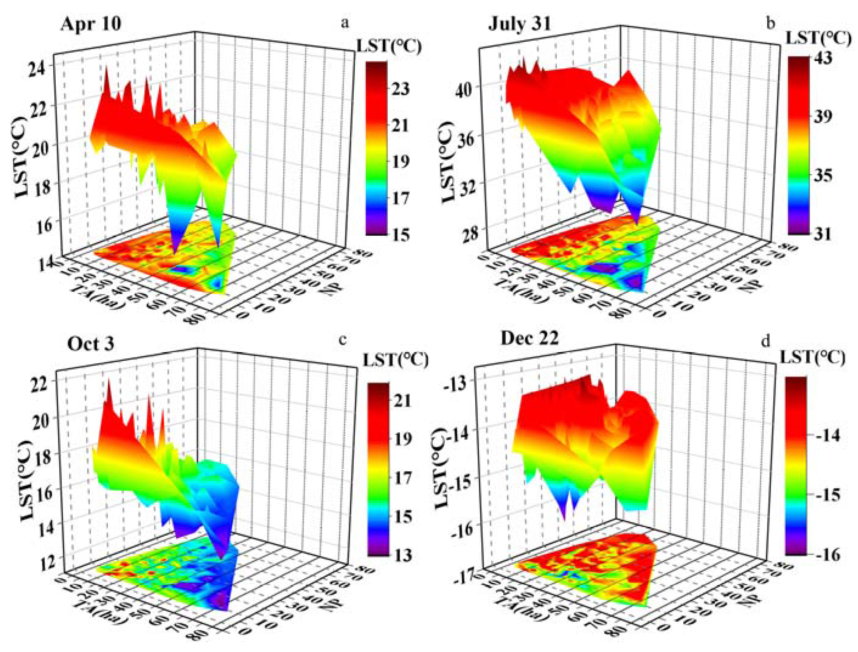
The negative relationship between urban green space areas (patch area, PA) and LST observed in this study is in agreement with previous studies [55,56,57]. A higher percentage of cover of green spaces leads to lower LST, and its negative effects on LST is more significant in summer than for the other three seasons. This may be due to summer having the most heterogeneous thermal environment and higher evapotranspiration of vegetation. Compared to the area of urban green patches, the negative effect of PERIM on LST is much weaker, indicating that it may not be an ideal metric to present information of green spaces for this study. We found that shape metrics PARA and SHAPE, compared to area metrics (PA, TA), were not very valuable in all seasons for assessing their relationship with LST. Moreover, the results suggested that a significant cooling effect occurrs when the TA is beyond a certain threshold. For example, in summer at the 0.5 km × 0.5 km scale, the value is approximately 5 ha. Therefore, based on the results, increasing the area of urban green spaces can effectively mitigate the UHI, and this was consistent with previous studies [38,58].
NDVI is typically used as the indicator of vegetation abundance to estimate the LST-vegetation relationship [21,59]. The results indicated that high values of NDVI for urban green spaces led to significantly lower temperatures for all seasons except winter at class level. The negative relationship between LST and NDVI was much stronger than that of LST and the area of urban green spaces. High values of NDVI were usually related to a good grow status of vegetation or more green space density. This is a clear indication that the status of vegetation (e.g., tree species, vegetation cover percentage) plays a vital role in cooling the urban thermal environment. In winter, the urban green spaces have little effect on the urban thermal environment, confirming that the status of vegetation does matter for cooling intensity. Therefore, in an urban environment without enough public space for green vegetation, increasing the NDVI (for example, vegetation canopy cover) is still an effective way to decrease LST.
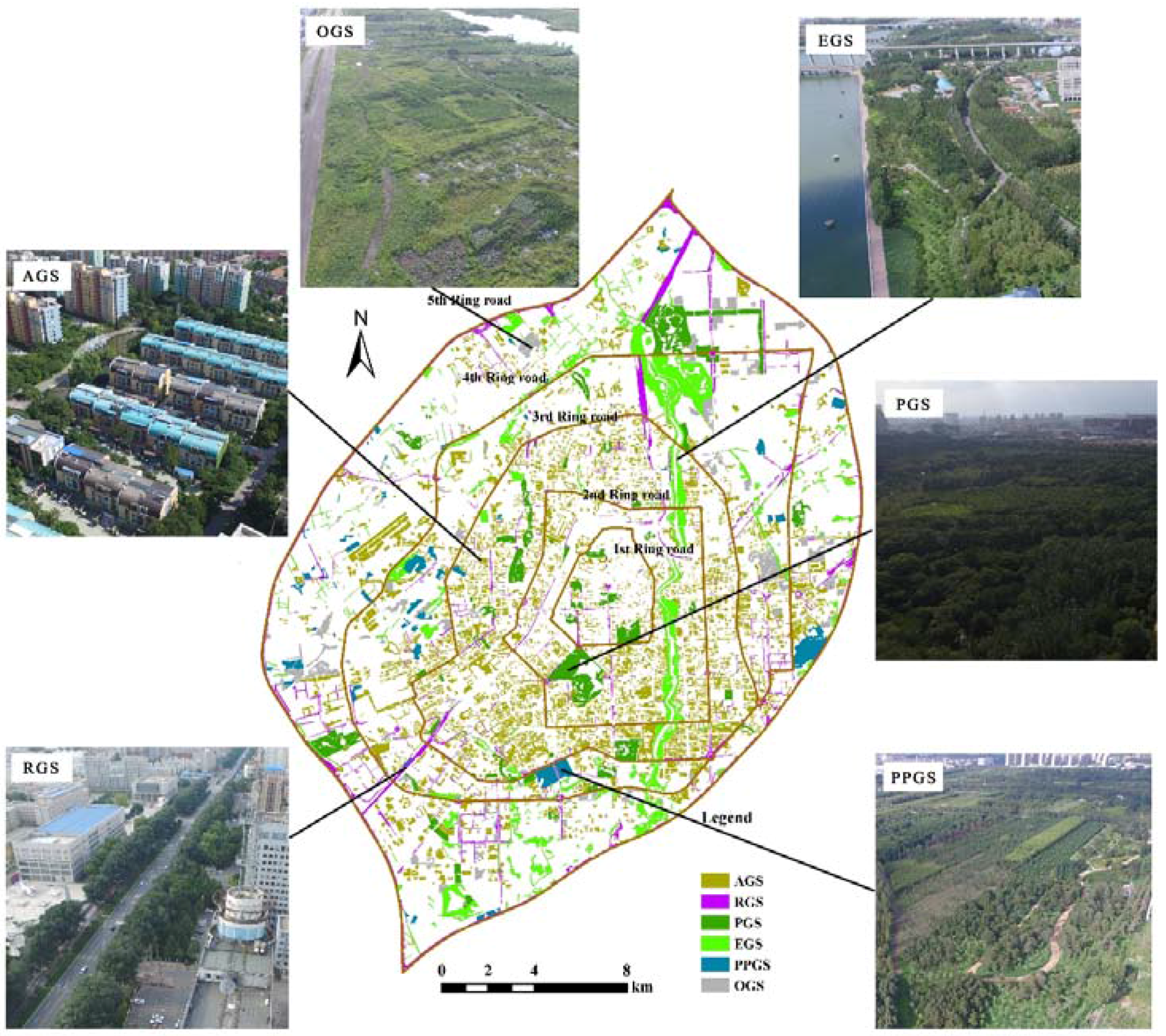
For different types of urban green spaces, PGS has a much lower temperature than the other types, while AGS and RGS usually have relative high temperatures. This may be due to several reasons: (1) the sizes of PGS sites were larger than other green space types, and there were more trees in parks; (2) the AGS patches were usually small and showed discrete distributions; and (3) the RGS sites were isolated and there were anthropogenic heat sources beside them, such as vehicles and buildings. As a result, by only considering the cooling intensity, if there is enough space, parks are a better choice than AGS and RGS for urban green infrastructure.
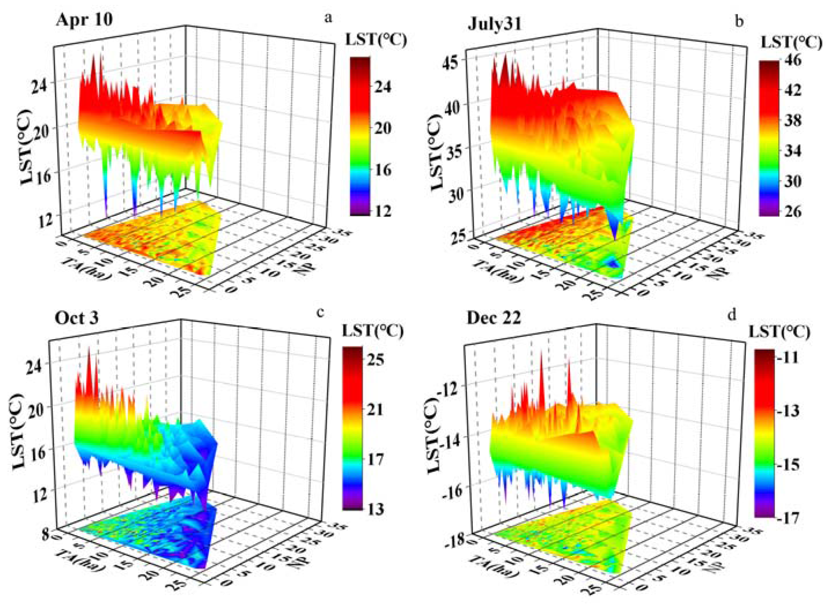
The whole study area was divided into small grids with a certain size, therefore the landscape-level metric NP rather than PD (patch density) was used to assess the spatial pattern of urban green spaces on LST. Our results showed that although the effect of the configuration of green spaces was not as strong as compositional features, it did play an important role in urban green space planning for regulating the micro-climate. For example, at the 1 km × 1 km scale, if a certain area of green space was to be arranged, how many patches should be considered? Our results showed that if the total area of green spaces was not large enough (approximately 20 ha in our case), the configuration has little influence. In summer, when the total area is larger than the threshold, for example, when the TA is between 20 and 30 ha in this study, with an increase in the number of patches, the LST tends to have few variations and even increases. However, when the patch number is larger than the threshold, the LST of the 1 km × 1 km grid will decrease significantly. Although when the TA is large enough on this scale, the NP has little effect on LST. As a result, the effects of NP on LST depends on the total area of urban green spaces and the season. Therefore, it still remains a challenge to assess how the NP can decrease LST in the most effective way. In addition, other landscape-level metrics, such as splitting index or connectance index could also be employed to investigate the effect of configuration in future studies. The splitting index is usually used to characterize landscape fragmentation in a geometric perspective and increases as the landscape is increasingly subdivided into smaller patches [60]. The connectance index is used as the proportion of functional joinings among all patches, where each pair of patches is either connected or not based on some criterion [43].

4.3. Limitations

This study has several limitations. First, only Landsat 8 TIR data were used to retrieve LST to characterize the spatial patterns of the urban thermal environment, thus the satellite overpass time was not synchronous with that of sparsely distributed meteorological stations. Due to the 30-m spatial resolution of TIRS data, the LST of some small green patches was influenced by surrounding urban areas. In addition, only one date was chosen to represent a season because there were insufficient daily or monthly images to meet the demand for retrieving LST. In addition, it is well known that different atmospheric conditions can affect the accuracy of the retrieved LST [
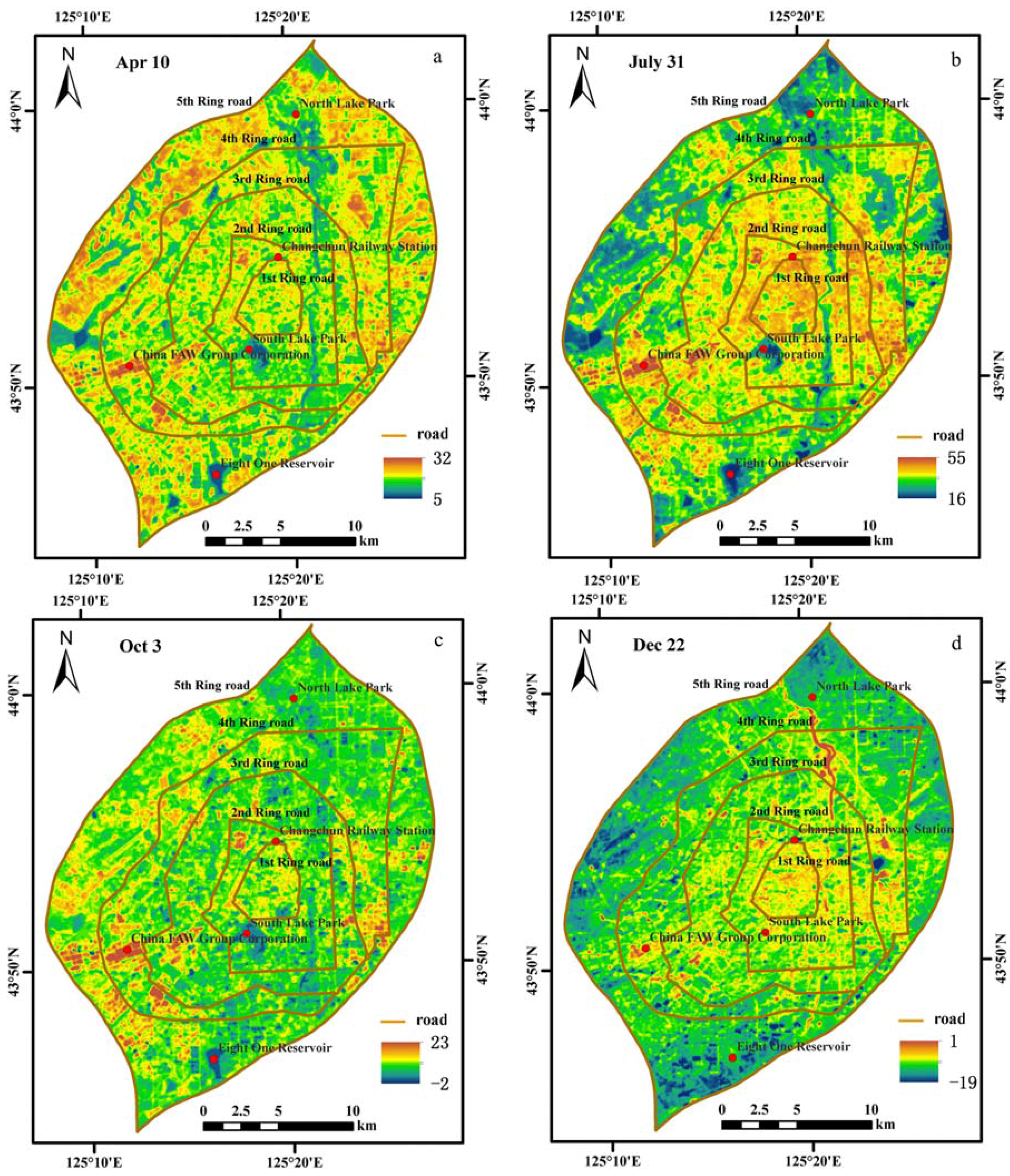
26]. However, these limitations were related to the difficulties in retrieving LST.
The second limitation is that bodies of water also play a very important role in cooling the LST [37,61]. For example, if bodies of water extensively exist in one analysis grid, the cooling effect of urban green spaces may be overestimated. However, the cooling effect of water was not considered in our study because we only sought to explore the effect of urban green spaces on thermal environments at the landscape level.
Finally, more attention is needed on the use of synchronous data from in-situ observations such as air temperature/humidity combined with high temporal resolution and long time span satellite data to have a better understanding of the cooling effect of urban green spaces produced by future studies. Researchers should interpret the results in comparison to previous studies and the working hypotheses. The findings and their implications should be further discussed in the broadest context possible, particularly to highlight future research directions.

5. Conclusions

Using Changchun, a cold temperate zone city, as a case study, this study investigated the effects of urban green spaces on urban thermal environments and their seasonal variations. With the support of multi-temporal Landsat OLI/TIRS images, high spatial resolution images GF-1, field data, and landscape ecology and comparative approaches were used to quantitatively examine the relationship between urban green spaces and LST. Our results showed the following:
(1)
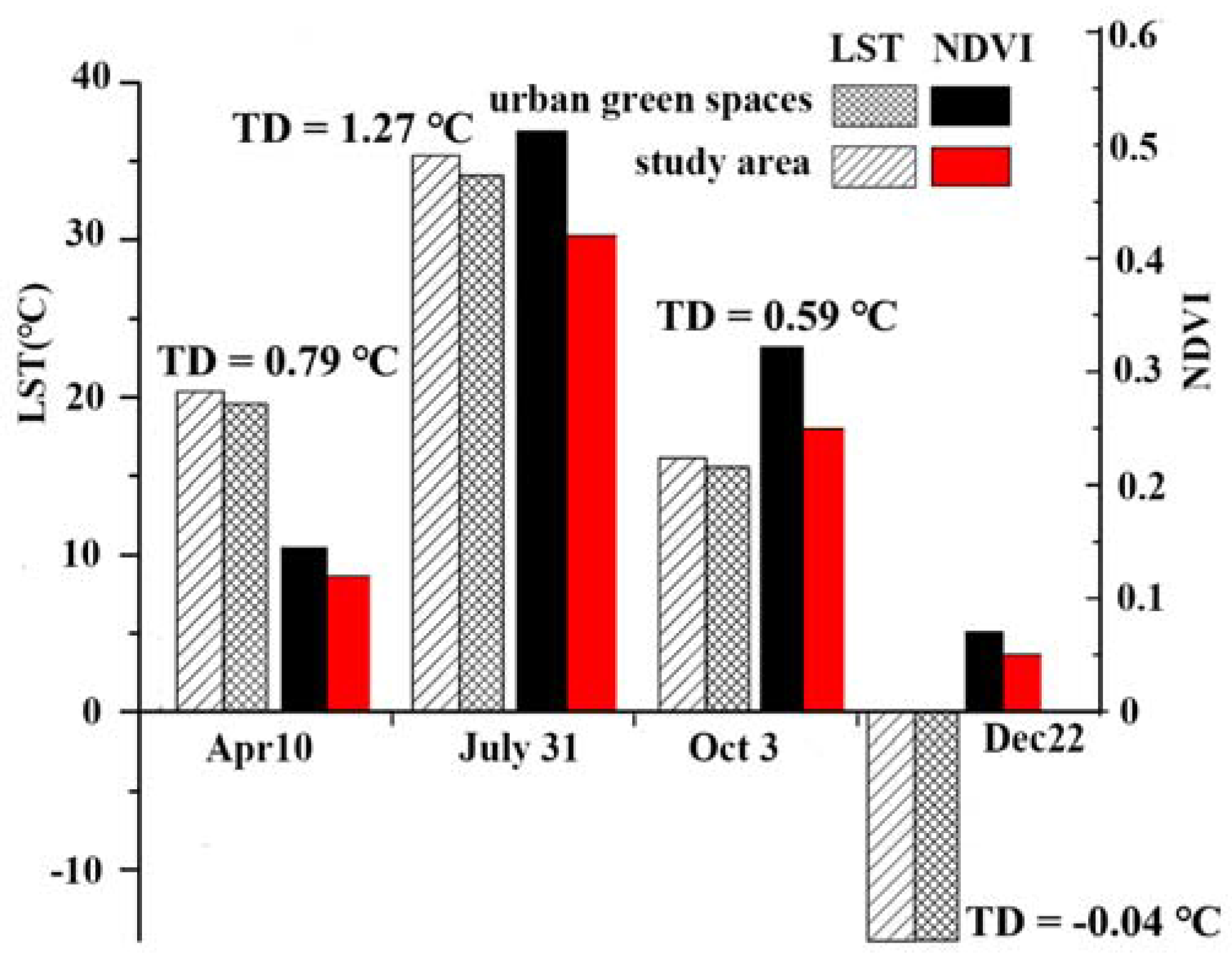
Urban green spaces have a significant cooling effect among all seasons except for winter, but the effects vary considerably among different seasons and green space types. The difference of LST between the urban green spaces and urban areas was large in the summer and small in the winter. The maximum value of the differences was 1.27 °C on 31 July. The lowest LST was found in PGS, while AGS and RGS have the highest LST among different green patches.
(2)
Compared to shape metrics such as PARA and SHAPE, the negative relationships between LST and the area and NDVI of urban green spaces were more significant. We found that every 10% increase in urban green spaces explained a 0.34 °C decrease in LST in summer at the 0.5 km × 0.5 km scale. Rather than increasing the area of green patches, increasing the NDVI (more woodland area and denser vegetation) is a better and more practicable approach for urban green planning.
(3)
Both the compositional features of urban green spaces and configuration can significantly affect LST. At certain spatial scales, for example, 1 km × 1 km, given a fixed area of urban green spaces, the number of green patches can increase or decrease the values of LST depending on if the number is larger than a threshold or not, and this threshold changes for each given area. For example, in our case, when the proportion of TA is between 20% and 40% in 100 ha, initially, the LST increases simultaneously with an increase in NP. When NP is larger than 40, however, the LST decreases.
This study has the potential to contribute to our understanding of how urban green spaces can mitigate urban heat island effects so that environmental problems may be resolved. The outcome of this study suggested that the process of cooling effects of urban green spaces differed among different seasons and green types, and it may provide insights for city planners and decision makers to forge sustainable urban strategies by considering the composition and configuration features of urban green spaces at the same time.

Acknowledgments

This research was supported by Youth Science fund project (41301466) approved by the National Natural Science Foundation of China. The authors wish to thank the Weather Bureau of Changchun for providing local meteorological data, the China Scholarship Council for funding Chaobin Yang to study and do scientific research in the USA, and the UNCC writing center and Elsevier’s language editing service for help with English editing.

Author Contributions

Chaobin Yang analyzed the data and wrote the paper; Xingyuan He and Shuwen Zhang conceived and designed the research; Ranghu Wang helped with obtaining ground reference data; Liping Chang, Kun Bu, and Jiuchun Yang helped with obtaining data and extracting urban spatial information; Lingxue Yu and Fengqin Yan assisted in data analysis and with editing the manuscript.

Conflicts of Interest

The authors declare no conflict of interest.

References

  1. Un, D. World Urbanization Prospects: The 2014 Revision; United Nations Department of Economics and Social Affairs, Population Division: New York, NY, USA, 2015. [Google Scholar]
  2. Rizwan, A.M.; Dennis, L.Y.; Chunho, L. A review on the generation, determination and mitigation of urban heat island. J. Environ. Sci. 2008, 20, 120–128. [Google Scholar] [CrossRef]
  3. Chen, X.-L.; Zhao, H.-M.; Li, P.-X.; Yin, Z.-Y. Remote sensing image-based analysis of the relationship between urban heat island and land use/cover changes. Remote Sens. Environ. 2006, 104, 133–146. [Google Scholar] [CrossRef]
  4. Wu, H.; Ye, L.-P.; Shi, W.-Z.; Clarke, K.C. Assessing the effects of land use spatial structure on urban heat islands using hj-1b remote sensing imagery in wuhan, china. Int. J. Appl. Earth Obs. Geoinform. 2014, 32, 67–78. [Google Scholar] [CrossRef]
  5. Arnberger, A.; Allex, B.; Eder, R.; Ebenberger, M.; Wanka, A.; Kolland, F.; Wallner, P.; Hutter, H.-P. Elderly resident’s uses of and preferences for urban green spaces during heat periods. Urban For. Urban Green. 2016, 21, 102–115. [Google Scholar] [CrossRef]
  6. Sun, Y.; Augenbroe, G. Urban heat island effect on energy application studies of office buildings. Energy Build. 2014, 77, 171–179. [Google Scholar] [CrossRef]
  7. Feizizadeh, B.; Blaschke, T. Examining urban heat island relations to land use and air pollution: Multiple endmember spectral mixture analysis for thermal remote sensing. IEEE J. Sel. Top. Appl. Earth Obs. Remote Sens. 2013, 6, 1749–1756. [Google Scholar] [CrossRef]
  8. Santamouris, M. The role of green spaces. In Energy and Climate in the Urban Built Environment; James & James: Springdale, AR, USA, 2001; pp. 145–159. [Google Scholar]
  9. Li, X.; Zhou, W.; Ouyang, Z. Relationship between land surface temperature and spatial pattern of greenspace: What are the effects of spatial resolution? Landsc. Urban Plan. 2013, 114, 1–8. [Google Scholar] [CrossRef]
  10. Wolch, J.R.; Byrne, J.; Newell, J.P. Urban green space, public health, and environmental justice: The challenge of making cities ‘just green enough’. Landsc. Urban Plan. 2014, 125, 234–244. [Google Scholar] [CrossRef]
  11. Park, J.; Kim, J.-H.; Lee, D.K.; Park, C.Y.; Jeong, S.G. The influence of small green space type and structure at the street level on urban heat island mitigation. Urban For. Urban Green. 2016, 21, 203–212. [Google Scholar] [CrossRef]
  12. Chang, C.-R.; Li, M.-H. Effects of urban parks on the local urban thermal environment. Urban For. Urban Green. 2014, 13, 672–681. [Google Scholar] [CrossRef]
  13. Akpinar, A.; Barbosa-Leiker, C.; Brooks, K.R. Does green space matter? Exploring relationships between green space type and health indicators. Urban For. Urban Green. 2016, 20, 407–418. [Google Scholar] [CrossRef]
  14. Derkzen, M.L.; Teeffelen, A.J.; Verburg, P.H. Review: Quantifying urban ecosystem services based on high-resolution data of urban green space: An assessment for rotterdam, The Netherlands. J. Appl. Ecol. 2015, 52, 1020–1032. [Google Scholar] [CrossRef]
  15. Zhang, B.; Gao, J.-X.; Yang, Y. The cooling effect of urban green spaces as a contribution to energy-saving and emission-reduction: A case study in Beijing, China. Build. Environ. 2014, 76, 37–43. [Google Scholar] [CrossRef]
  16. Chen, X.; Su, Y.; Li, D.; Huang, G.; Chen, W.; Chen, S. Study on the cooling effects of urban parks on surrounding environments using landsat tm data: A case study in guangzhou, southern china. Int. J. Remote Sens. 2012, 33, 5889–5914. [Google Scholar] [CrossRef]
  17. Shashua-Bar, L.; Hoffman, M.E. Vegetation as a climatic component in the design of an urban street: An empirical model for predicting the cooling effect of urban green areas with trees. Energy Build. 2000, 31, 221–235. [Google Scholar] [CrossRef]
  18. Hamada, S.; Ohta, T. Seasonal variations in the cooling effect of urban green areas on surrounding urban areas. Urban For. Urban Green. 2010, 9, 15–24. [Google Scholar] [CrossRef]
  19. Susca, T.; Gaffin, S.; Dell’Osso, G. Positive effects of vegetation: Urban heat island and green roofs. Environ. Pollut. 2011, 159, 2119–2126. [Google Scholar] [CrossRef] [PubMed]
  20. Bertram, C.; Rehdanz, K. The role of urban green space for human well-being. Ecol. Econ. 2015, 120, 139–152. [Google Scholar] [CrossRef]
  21. Weng, Q.; Lu, D.; Schubring, J. Estimation of land surface temperature—Vegetation abundance relationship for urban heat island studies. Remote Sens. Environ. 2004, 89, 467–483. [Google Scholar] [CrossRef]
  22. Streutker, D.R. Satellite-measured growth of the urban heat island of houston, texas. Remote Sens. Environ. 2003, 85, 282–289. [Google Scholar] [CrossRef]
  23. Weng, Q.; Quattrochi, D.A. Thermal remote sensing of urban areas: An introduction to the special issue. Remote Sens. Environ. 2006, 104, 119–122. [Google Scholar] [CrossRef]
  24. Weng, Q. Thermal infrared remote sensing for urban climate and environmental studies: Methods, applications, and trends. ISPRS J. Photogramm. Remote Sens. 2009, 64, 335–344. [Google Scholar] [CrossRef]
  25. Dash, P.; Göttsche, F.-M.; Olesen, F.-S.; Fischer, H. Land surface temperature and emissivity estimation from passive sensor data: Theory and practice-current trends. Int. J. Remote Sens. 2002, 23, 2563–2594. [Google Scholar] [CrossRef]
  26. Li, Z.-L.; Tang, B.-H.; Wu, H.; Ren, H.; Yan, G.; Wan, Z.; Trigo, I.F.; Sobrino, J.A. Satellite-derived land surface temperature: Current status and perspectives. Remote Sens. Environ. 2013, 131, 14–37. [Google Scholar] [CrossRef]
  27. Voogt, J.A.; Oke, T. Effects of urban surface geometry on remotely-sensed surface temperature. Int. J. Remote Sens. 1998, 19, 895–920. [Google Scholar] [CrossRef]
  28. Voogt, J.A.; Oke, T.R. Thermal remote sensing of urban climates. Remote Sens. Environ. 2003, 86, 370–384. [Google Scholar] [CrossRef]
  29. Liu, L.; Zhang, Y. Urban heat island analysis using the landsat tm data and aster data: A case study in hong kong. Remote Sens. 2011, 3, 1535–1552. [Google Scholar] [CrossRef]
  30. Rogan, J.; Ziemer, M.; Martin, D.; Ratick, S.; Cuba, N.; DeLauer, V. The impact of tree cover loss on land surface temperature: A case study of central massachusetts using landsat thematic mapper thermal data. Appl. Geogr. 2013, 45, 49–57. [Google Scholar] [CrossRef]
  31. Roy, D.P.; Wulder, M.; Loveland, T.; Woodcock, C.; Allen, R.; Anderson, M.; Helder, D.; Irons, J.; Johnson, D.; Kennedy, R. Landsat-8: Science and product vision for terrestrial global change research. Remote Sens. Environ. 2014, 145, 154–172. [Google Scholar] [CrossRef]
  32. Cao, X.; Onishi, A.; Chen, J.; Imura, H. Quantifying the cool island intensity of urban parks using aster and ikonos data. Landsc. Urban Plan. 2010, 96, 224–231. [Google Scholar] [CrossRef]
  33. Connors, J.P.; Galletti, C.S.; Chow, W.T. Landscape configuration and urban heat island effects: Assessing the relationship between landscape characteristics and land surface temperature in phoenix, arizona. Landsc. Ecol. 2013, 28, 271–283. [Google Scholar] [CrossRef]
  34. Myint, S.W.; Wentz, E.A.; Brazel, A.J.; Quattrochi, D.A. The impact of distinct anthropogenic and vegetation features on urban warming. Landsc. Ecol. 2013, 28, 959–978. [Google Scholar] [CrossRef]
  35. Li, J.; Song, C.; Cao, L.; Zhu, F.; Meng, X.; Wu, J. Impacts of landscape structure on surface urban heat islands: A case study of shanghai, china. Remote Sens. Environ. 2011, 115, 3249–3263. [Google Scholar] [CrossRef]
  36. Chen, A.; Yao, L.; Sun, R.; Chen, L. How many metrics are required to identify the effects of the landscape pattern on land surface temperature? Ecol. Indic. 2014, 45, 424–433. [Google Scholar] [CrossRef]
  37. Chen, A.; Yao, X.A.; Sun, R.; Chen, L. Effect of urban green patterns on surface urban cool islands and its seasonal variations. Urban For. Urban Green. 2014, 13, 646–654. [Google Scholar] [CrossRef]
  38. Zhibin, R.; Haifeng, Z.; Xingyuan, H.; Dan, Z.; Xingyang, Y. Estimation of the relationship between urban vegetation configuration and land surface temperature with remote sensing. J. Indian Soc. Remote Sens. 2015, 43, 89–100. [Google Scholar] [CrossRef]
  39. Gustafson, E.J. Quantifying landscape spatial pattern: What is the state of the art? Ecosystems 1998, 1, 143–156. [Google Scholar] [CrossRef]
  40. McGarigal, K.; Marks, B.J. Spatial Pattern Analysis Program for Quantifying Landscape Structure; PNW-GTR-351; US Department of Agriculture, Forest Service, Pacific Northwest Research Station: Portland, OR, USA, 1995.
  41. Zhou, X.; Wang, Y.-C. Spatial-temporal dynamics of urban green space in response to rapid urbanization and greening policies. Landsc. Urban Plan. 2011, 100, 268–277. [Google Scholar] [CrossRef]
  42. Zhou, W.; Qian, Y.; Li, X.; Li, W.; Han, L. Relationships between land cover and the surface urban heat island: Seasonal variability and effects of spatial and thematic resolution of land cover data on predicting land surface temperatures. Landsc. Ecol. 2014, 29, 153–167. [Google Scholar] [CrossRef]
  43. McGarigal, K.; Cushman, S.A.; Neel, M.C.; Ene, E. Fragstats: Spatial Pattern Analysis Program for Categorical Maps. 2002. Available online: http://www.umass.edu/landeco/research/fragstats/fragstats.html (accessed on 3 July 2017).
  44. Yang, C.; He, X.; Yan, F.; Yu, L.; Bu, K.; Yang, J.; Chang, L.; Zhang, S. Mapping the influence of land use/land cover changes on the urban heat island effect—A case study of Changchun, China. Sustainability 2017, 9, 312. [Google Scholar] [CrossRef]
  45. Qin, Z.-h.; Karnieli, A.; Berliner, P. A mono-window algorithm for retrieving land surface temperature from landsat tm data and its application to the israel-egypt border region. Int. J. Remote Sens. 2001, 22, 3719–3746. [Google Scholar] [CrossRef]
  46. Rozenstein, O.; Qin, Z.; Derimian, Y.; Karnieli, A. Derivation of land surface temperature for landsat-8 tirs using a split window algorithm. Sensors 2014, 14, 5768–5780. [Google Scholar] [CrossRef] [PubMed]
  47. Sobrino, J.A.; Jiménez-Muñoz, J.C.; Sòria, G.; Romaguera, M.; Guanter, L.; Moreno, J.; Plaza, A.; Martínez, P. Land surface emissivity retrieval from different vnir and tir sensors. In Proceedings of the IEEE Transactions on Geoscience and Remote Sensing, New York, NY, USA, 2008; pp. 316–327. [Google Scholar]
  48. Sobrino, J.; Raissouni, N.; Li, Z.-L. A comparative study of land surface emissivity retrieval from noaa data. Remote Sens. Environ. 2001, 75, 256–266. [Google Scholar] [CrossRef]
  49. Yang, L.; Cao, Y.; Zhu, X.; Zeng, S.; Yang, G.; He, J.; Yang, X. Land surface temperature retrieval for arid regions based on landsat-8 tirs data: A case study in shihezi, northwest china. J. Arid Land 2014, 6, 704–716. [Google Scholar] [CrossRef]
  50. Maimaitiyiming, M.; Ghulam, A.; Tiyip, T.; Pla, F.; Latorre-Carmona, P.; Halik, Ü.; Sawut, M.; Caetano, M. Effects of green space spatial pattern on land surface temperature: Implications for sustainable urban planning and climate change adaptation. ISPRS J. Photogramm. Remote Sens. 2014, 89, 59–66. [Google Scholar] [CrossRef]
  51. Turner, M.G. Landscape ecology: The effect of pattern on process. Annu. Rev. Ecol. Syst. 1989, 20, 171–197. [Google Scholar] [CrossRef]
  52. Lee, S.-W.; Hwang, S.-J.; Lee, S.-B.; Hwang, H.-S.; Sung, H.-C. Landscape ecological approach to the relationships of land use patterns in watersheds to water quality characteristics. Landsc. Urban Plan. 2009, 92, 80–89. [Google Scholar] [CrossRef]
  53. Riva-Murray, K.; Riemann, R.; Murdoch, P.; Fischer, J.M.; Brightbill, R. Landscape characteristics affecting streams in urbanizing regions of the delaware river basin (New Jersey, New York, and Pennsylvania, US). Landsc. Ecol. 2010, 25, 1489–1503. [Google Scholar] [CrossRef]
  54. Yuan, F.; Bauer, M.E. Comparison of impervious surface area and normalized difference vegetation index as indicators of surface urban heat island effects in landsat imagery. Remote Sens. Environ. 2007, 106, 375–386. [Google Scholar] [CrossRef]
  55. Carlson, T.N.; Gillies, R.R.; Perry, E.M. A method to make use of thermal infrared temperature and ndvi measurements to infer surface soil water content and fractional vegetation cover. Remote Sens. Rev. 1994, 9, 161–173. [Google Scholar] [CrossRef]
  56. Liang, B.; Weng, Q. Assessing urban environmental quality change of indianapolis, united states, by the remote sensing and gis integration. IEEE J. Sel. Top. Appl. Earth Obs. Remote Sens. 2011, 4, 43–55. [Google Scholar] [CrossRef]
  57. Tran, H.; Uchihama, D.; Ochi, S.; Yasuoka, Y. Assessment with satellite data of the urban heat island effects in asian mega cities. Int. J. Appl. Earth Obs. Geoinf. 2006, 8, 34–48. [Google Scholar] [CrossRef]
  58. Senanayake, I.; Welivitiya, W.; Nadeeka, P. Urban green spaces analysis for development planning in Colombo, Sri Lanka, utilizing THEOS satellite imagery—A remote sensing and GIS approach. Urban For. Urban Green. 2013, 12, 307–314. [Google Scholar] [CrossRef]
  59. Gallo, K.; McNab, A.; Karl, T.; Brown, J.; Hood, J.; Tarpley, J. The use of a vegetation index for assessment of the urban heat island effect. Remote Sens. 1993, 14, 2223–2230. [Google Scholar] [CrossRef]
  60. Jaeger, J.A. Landscape division, splitting index, and effective mesh size: New measures of landscape fragmentation. Landsc. Ecol. 2000, 15, 115–130. [Google Scholar] [CrossRef]
  61. Feyisa, G.L.; Dons, K.; Meilby, H. Efficiency of parks in mitigating urban heat island effect: An example from addis ababa. Landsc. Urban Plan. 2014, 123, 87–95. [Google Scholar] [CrossRef]
Figure 1. Location of Changchun city and its GF-1 image (2-m spatial resolution).
Forests 08 00153 g001
Figure 2. Spatial distribution of six types of urban green spaces in Changchun.
Forests 08 00153 g002
Figure 3. Lands surface temperature (°C) of (a) 10 April; (b) 31 July; (c) 3 October, and (d) 22 December in 2014.
Forests 08 00153 g003
Figure 4. The LST and NDVI of urban green spaces and the overall study area across four dates.
Forests 08 00153 g004
Figure 5. Grid map of landscape metrics: (a) TA, 0.5 × 0.5 km; (b) TA, 1 × 1 km; (c) NP, 0.5 × 0.5 km; (d) NP, 1 × 1 km.
Forests 08 00153 g005
Figure 6. Scatter plots of LST with TA across different seasons: (a) 10 April; (b) 31 July; (c) 3 October, and (d) 22 December in 2014 at 0.5 × 0.5 km scale.
Forests 08 00153 g006
Figure 7. Scatter plots of LST with TA across different seasons: (a) 10 April; (b) 31 July; (c) 3 October, and (d) 22 December in 2014 at 1 × 1 km scale.
Forests 08 00153 g007
Figure 8. The 3-D images of TA, NP, and LST across different seasons: (a) 10 April; (b) 31 July; (c) 3 October; and (d) 22 December in 2014 at 0.5 × 0.5 km scale.
Forests 08 00153 g008
Figure 9. The 3-D images of TA, NP, and LST across different seasons: (a) 10 April; (b) 31 July; (c) 3 October; and (d) 22 December in 2014 at 1 × 1 km scale.
Forests 08 00153 g009
Table 1. Urban green spaces types and its descriptions.
Types and AbbreviationDescriptions
Attached Green Spaces, AGSgreen spaces located in commercial , residential areas and institutions
Road Green Spaces, RGSgreen spaces on the sides of road, usually shown as belt bands
Park Green Spaces, PGStheme parks, comprehensive parks, forest parks, and other parks
Productive Plantation Green Spaces, PPGSnursery gardens, featuring saplings, flowers, and plants
Ecological Green Spaces, EGSwindbreaks, sediment control, used for environment protection
Other Green Spaces, OGSother green spaces types not belonging to any of the above types
Table 2. Landscape metrics used in this study to describe urban green spaces.
Metrics and AbbreviationDescriptions and Calculations
patch area, PAequals the area (m2 or hectare) of the patch, PA > 0, without limit
patch perimeter, PERIMequals the perimeter (m) of the patch, PERIM > 0, without limit
perimeter-area ratio, PARAequals the ratio of the patch perimeter (m) to area (m2). PARA = PERIM/PA, PARA > 0, without limit
shape index, SHAPEequals the ratio of the patch perimeter (m) to area (m2). SHAPE = 0.25 PERIM/√PA, SHAPE ≥ 1
total area, TAequals the sum of the areas (m2) of all patches of the corresponding patch type or the landscape, TA > 0, without limit
number of patches, NPequals the number of patches of the corresponding patch type (class), NP ≥ 1, without limit
Table 3. The statistical information of the urban green spaces. TA: total area.
TypesMean Patch Area (ha)TA (km2)Percentage Area (%)
AGS0.6543.2437.3
RGS1.7317.0114.7
PGS14.5615.0212.9
EGS6.4422.3519.3
PPGS9.366.185.3
OGS6.9912.0410.4
All1.39115.84100
Table 4. The statistical information of the land surface temperature (LST) among the four seasons.
DateMax (°C)Min (°C)Mean (°C)SD (°C)
10 April31.865.2820.372.14
31 July54.5316.5535.373.87
3 October32.09−2.5616.351.77
22 December0.81−19.62−14.561.00
Table 5. Spearman’s rho correlation coefficients between LST and patch-level metrics, normalized differential vegetation index (NDVI) on 31 July 2014.
PA (ha)PAPERIMPARASHAPENDVI
0.36–0.81 (n = 1850)−0.084 **−0.0410.038−0.003−0.328 **
0.81–1.44 (n = 759)−0.094 **−0.072 *−0.023−0.048−0.361 **
1.44–5.76 (n = 929)−0.217 **−0.088 **0.116 **0.013−0.503 **
5.76–9 (n = 155)−0.0770.0210.0640.039−0.542 **
9–15.2 (n = 124)−0.024−0.099−0.084−0.093−0.654 **
>15.2 (n = 104)−0.189−0.235 *−0.086−0.196 *−0.537 **
* Correlation is significant at the 0.05 level (two-tailed); ** Correlation is significant at the 0.01 level (two-tailed).
Table 6. The best fit multiple regression model showing relationships between LST and patch-level metrics, NDVI on 31 July 2014. (N = 3921, Adj. R2 = 0.335).
Variables EnteredStandardized Coefficients (Beta)Std. Errorp-Value
Intercept (40.515) 0.1980.000
NDVI−0.4840.3770.000
PERIM−0.0430.0000.038
PARA0.1251.6870.000
SHAPE−0.1320.0890.000
Table 7. Average LST and standard deviation over different urban green spaces in 2014.
Dates10 April31 July3 October22 December
LST (°C)MeanSDNDVIMeanSDNDVIMeanSDNDVIMeanSDNDVI
AGS20.141.370.1335.372.120.4515.761.350.28−14.410.680.05
RGS20.191.210.1434.312.550.5115.851.310.32−14.560.770.07
PGS18.651.550.1732.072.180.5414.931.110.39−14.610.720.09
EGS18.752.020.1532.132.460.5815.240.840.34−14.371.180.08
PPGS19.721.440.1833.012.130.6215.090.910.41−15.320.590.11
OGS20.181.800.1433.822.900.5616.101.010.28−14.680.690.08

